Synthesizing Neural Network Controllers with Probabilistic Model ...

Synthesizing Neural Network Controllers with Probabilistic Model-Based Reinforcement Learning

arXiv:1803.02291v1 [cs.RO] 6 Mar 2018

Juan Camilo Gamboa Higuera, David Meger, and Gregory Dudek Abstract— We present an algorithm for rapidly learning controllers for robotics systems. The algorithm follows the model-based reinforcement learning paradigm, and improves upon existing algorithms; namely Probabilistic learning in Control (PILCO) and a sample-based version of PILCO with neural network dynamics (Deep-PILCO). We propose training a neural network dynamics model using variational dropout with truncated Log-Normal noise. This allows us to obtain a dynamics model with calibrated uncertainty, which can be used to simulate controller executions via rollouts. We also describe set of techniques, inspired by viewing PILCO as a recurrent neural network model, that are crucial to improve the convergence of the method. We test our method on a variety of benchmark tasks, demonstrating data-efficiency that is competitive with PILCO, while being able to optimize complex neural network controllers. Finally, we assess the performance of the algorithm for learning motor controllers for a six legged autonomous underwater vehicle. This demonstrates the potential of the algorithm for scaling up the dimensionality and dataset sizes, in more complex control tasks.

I. I NTRODUCTION Model-based reinforcement learning (RL) is an attractive framework for addressing the synthesis of controllers for robots of all kinds due to its promise of data-efficiency. By using experience data to produce state-transition dynamics models via fitting, an RL agent can search for good controllers, using these models to evaluate policies in simulation. This allows for minimizing costly trials on a target robot platform. Minimizing interactions, however, means that experience datasets will often not be large enough to obtain accurate dynamics models. Bayesian models are very helpful in this situation. Instead of requiring an accurate model, the robotic agent may keep track of a distribution over dynamics models that are compatible with its experience. Evaluating a controller then involves quantifying its performance over the dynamics model distribution. To improve its chances of working in the real world an effective controller should perform well, on average, when drawing a model from this distribution. Two successful applications of this idea are the PILCO 1 and Deep-PILCO algorithms. PILCO [1] uses Gaussian Process (GP) models to fit one-step dynamics and networks of radial basis functions (RBFs) for feedback policies. PILCO has been shown to perform very well with little data in benchmark simulated tasks and on real robots [1]. We have used PILCO successfully for synthesizing swimming The authors are part of the Center for Intelligent Machines and the School of Computer Science, McGill University, Montreal, Canada. This work was supported by NSERC through funding for the NSERC Canadian Field Robotics Network

{gamboa,dmeger,dudek}@cim.mcgill.ca 1 Probabilistic

Inference and Learning for COntrol

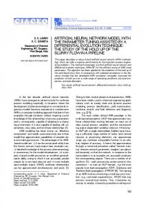
Fig. 1: The AQUA robot executing a 6-leg knife edge maneuver. The robot starts in its resting position and must swim forward at a constant depth while stabilizing a roll angle of 90 degrees. The sequence of images illustrates the controller learned with the methods described in this work. controllers for an underwater swimming robot [2]. However, PILCO is computationally expensive. Model fitting scales O(Dn3 ) and long-term predictions scale O(D3 n2 ), where n is the dataset size and D is the number of state dimensions, limiting its applicability only to scenarios with small datasets and a small number of dimensions. Deep-PILCO [3] aims to address these limitations by employing Bayesian Neural Networks (BNN), implemented using binary dropout [4], [5]. Deep-PILCO uses BNNs to fit a dynamics model, and performs a sampling-based procedure for simulation. Policy search and model learning are done via stochastic gradient optimization: computations with linear scaling in the dataset size and state dimensionality. DeepPILCO has been shown to result in better performing policies for the cart-pole swing-up benchmark task, but show reduced data efficiency when compared with PILCO on the same task. In this work, we extend on the results of [3]. We demonstrate that Deep-PILCO can match the data efficiency of PILCO on the cart-pole swing-up task with a small number of heuristics to stabilize optimization. We demonstrate that using neural network controllers improves the data efficiency of Deep-PILCO. We also show that using Log-Normal multiplicative noise [6] removes the need for searching for the appropriate dropout rate, and outperforms the original version of Deep-PILCO with binary dropout on the cartdouble pendulum swing-up task. II. R ELATED W ORK Dynamics models have long been a core element in the modeling and control of robotic systems. For example,

trajectory optimization approaches [7], [8], [9] can produce highly effective controllers for complex robotic systems when precise analytical models are available. For complex and stochastic systems such as swimming robots, classical models are less reliable. In these cases, either performing online system identification [10] or learning complete dynamics models from data has proven to be effective, and can be integrated tightly with model-based control schemes [11], [12], [13], [14]. Multiple authors have recently considered the use of Deep RL methods to learn continuous control tasks up to an including full-body control of acrobatic humanoid characters [15]. These methods do not assume a known reward function, and thus estimate the value of each action only from experience. Along with their model-free nature, this factor results in much lower data efficiency compared with the methods we consider here, but there are ongoing efforts to connect modelbased and model-free approaches [16]. The most similar works to our own are those which utilize uncertain learned dynamics models for policy optimization. Locally linear controllers can be learned in this fashion, for example by extending the classical Differential Dynamic Programming (DDP) [17] method or Iterative LQG [18] to apply over trajectory distributions. For more complex robots, it is desirable to learn complex non-linear policies using the predictions of learned dynamics. Considering Gaussian Process dynamics, a gradient-free policy search approach, Black-DROPS [19], has recently shown promising performance along with the gradient-based PILCO [1]. As yet, we are only aware of Bayesian Neural Networks being optimized in the model-learning loop within Deep PILCO [3], which is the method we directly improve upon in this work. Our approach is the first model-based RL approach to utilize BNNs for both the dynamics as well as the policy network. III. P ROBLEM S TATEMENT

𝐱𝑡 𝐱𝑡

𝜋𝜃 policy

𝑓𝜓 𝐮𝑡

model

Fig. 2: An overview diagram of the components used for sampling 27

simulated trajectories. When both the policy and the model are implemented with neural networks, this model is effectively a simple recurrent neural network (RNN); with the same problems with long-term dependencies as traditional RNNs.

IV. M ETHODS A. Learning a dynamics model A key to data-efficiency is avoiding model bias, which happens when optimizing the objective in Equation 1 with a model that makes bad predictions high confidence. Bayesian neural networks (BNN) avoid model bias by finding a posterior distributions over the parameters of the network. Given a network fψ , with parameters ψ, and a training dataset D = {X, Y} we would like to use the posterior p(ψ|X, Y) to make predictions at novel test points. This distribution represents how certain we are about the true value of the parameters, which inRturn induces uncertainty on the model predictions: p(y) = p(y|fψ )p(ψ|x, X, Y)dψ, where y is the estimated predictions for a test point x. Using the true posterior for predictions on a neural network is intractable. Fortunately, various methods based on variational inference have been proposed, which use a tractable approximate posterior and Monte Carlo inference for predictions [20], [21], [5], [22], [23]. Fitting is done by minimizing the Kullback-Leibler (KL) divergence between the true and the approximate posterior. In most of these variational approximations, the objective function for fitting the model is of the form L(ψ) = −LD (ψ) + DKL (q(ψ)|p(ψ)

We consider target systems that can be modeled with discrete-time first-order dynamics xt+1 = f (xt , ut ), where f is unknown, with states xt ∈ RD and controls ut ∈ RU , indexed by time-step t. The goal is to find the parameters θ of a control policy πθ that minimize a state-dependent cost function c accumulated over a finite time horizon H, (H ) X (1) arg min J(θ) = Eτ c(xt ) θ . θ

i=1

The expectation is due to not knowing the true dynamics f , which induces a distribution over trajectories p(τ ) = p(x1 , u1 , ..., xH , uH ). The objective could be estimated by black-box optimization or likelihood ratio method, obtaining trajectory samples directly from the target system. However, such methods are known to require a large number of evaluations, which may be impractical for applications on physical robot systems. An alternative is to use experience to fit an estimated model, and use the model to evaluate the objective in Equation 1.

𝐱𝑡+1

(2)

where LD is the likelihood of the data, q(ψ) is the approximate posterior and p(ψ) is some user-defined prior on the parameters. To fit the dynamics model, we build the dataset D of tuples h(xt , ut ), ∆t i; where (xt , ut ) ∈ RD+U are the state-action pairs that we use as input to the dynamics models, and ∆t = xt − xt−1 ∈ RX are the changes in state observed after applying action ut at state xt . Fitting the model is done by minimizing The objective 2 via stochastic gradient descent. In this work, we evaluate the use of BNN models based on the dropout approximation [5] and the truncated Log-Normal approximation [6]. B. Policy optimization To estimate the objective function in Equation 1, we base our approach on the Deep-PILCO method [3]. This consists on performing forward simulations using the model fψ , as illustrated in Figure 2. Specifically, samples from p(τ ) are obtained by first sampling an ensemble of K dynamics

(k)

(k)

models f˜ψ and K initial state particles x1 , with k = 1, ..., K. These states are fed into the policy to obtain a set (k) of corresponding actions u1 . The states and actions are used (k) by the corresponding model f˜ψ to produce a set of particles (k) for the next state x2 . Finally, the particles are resampled (k) by fitting a Gaussian distribution to the particles x2 , and sampling K new particles from this Gaussian. The process is repeated for the next states until reaching time step H. This procedure can be summarized by the following model: (k) (k) x1 ∼ p(x1 ), f˜ψ ∼ q(ψ),   (k) (k) (k) (k) (k) (k) (k) ut ∼ πθ ut |xt , yt+1 ∼ p(xt+1 |xt , ut , fψ(k) ), (k)

(k)

xt+1 ∼ N (xt+1 |µyt , Σyt ). (3) Finally, the objective is approximated via Monte Carlo integration arg min θ

K X H X (k) ˜ = 1 c(xt ). J(θ) K i=1

(4)

k=1

We optimize this objective via stochastic gradient descent since the task-dependent cost is assumed to be differentiable, and policy evaluations and dynamics model predictions are differentiable. V. I MPROVEMENTS TO D EEP -PILCO In this section we enumerate the changes we have done to the Deep-PILCO, and that were crucial for improving its data-efficiency and obtaining the results we describe in the following sections. A. Common random numbers (CRN) and PEGASUS policy evaluation The convergence of Deep-PILCO is highly dependent ˆ on the variance of the estimated gradient ∇θ J(θ) = PK (k) 1 (k) ˆ ∇ J(θ| f , x ). The variance of this gradient is, θ 1 k K among other things, dependent on p(x1 ), the random numbers used for Monte Carlo integration, and the number of particles K. In our initial experiments we increased K from 10 to 100, and found it to improve convergence with small penalty on running time. Increasing the number of particles also enables us to further reduce variance by using common random numbers (CRN). The generative model in Eq. 3, implemented with BNNs in Deep-PILCO, relies on the re-parameterization trick [21] to propagate policy gradients over the simulation horizon. If we provide the random numbers for the policy evaluation step of Deep-PILCO, we obtain a variant of the PEGASUS2 algorithm [24]. This approach requires intermediate moment-matching and re-sampling steps. To reduce the impact of biases from deterministic policy evaluations, we resample the random numbers after each trial, but they remain fixed during the policy optimization phase. 2 Policy

Evaluation-of-Goodness And Search Using Scenarios

B. Gradient Clipping As noted in [3], the recurrent application of BNNs to implement the generative model in Eq. 3 can be interpreted as a Recurrent Neural Network (RNN) model. As such, DeepPILCO is prone to suffer from vanishing and exploding gradients [25], especially when dealing with tasks that require long time horizon or very deep models for the dynamics and policy. Although numerous techniques have been proposed in the RNN literature, we found the gradient clipping strategy to be effective in our experiments; as shown in Figure 6b. C. Training neural network controllers While Deep-PILCO had been limited to training singlelayer Radial Basis Function policies, the application of gradient clipping and CRNs allows stable training of deep neural network policies, opening the door for richer behaviors. We found that adding dropout regularization to the policy networks improves performance. During policy evaluation, we sample from policies with a similar scheme to that used for dynamics models. For each particle, we sample one dynamics model and one policy, and keep them fixed during policy evaluation. This can be viewed as attempting to learn a distribution of controllers that are likely to perform well over plausible dynamic models. We decided to make the policy stochastic during execution, by using a single dropout sample of the policy at every time step. This provides a limited amount of exploration, which we found beneficial, in particular, for the double cart-pole swing-up task. D. BNNs with Log-Normal multiplicative noise Deep-PILCO with binary dropout requires tuning the dropout probability to a value appropriate for the model size. We experimented with other BNN models [26], [22], [6] to enable learning the dropout probabilities from data. The best performing method in our experiments was using Log-Normal dropout with a truncated log-uniform prior LogU[−10,0] . The multiplicative noise is constrained to values between 0 and 1 [6]. Other methods we may explore in the future include Concrete Dropout [23] and Beta distributed multiplicative noise. VI. R ESULTS In our experiments, we use the ADAM algorithm [27] for model fitting and policy optimization, with the default parameters suggested by the authors. We report the best results we obtained after minimal manual hyper-parameter tuning. A. Cart-pole and double pendulum on cart swing-up tasks We tested the improvements, described in Section III, on two benchmark scenarios: swinging up and stabilizing an inverted pendulum on a cart, and swinging up and stabilizing a double pendulum on a cart. These tasks are illustrated in Figure 3. The first task was meant to compare performance on the same experimental setup as [3]. We chose the second scenario to compare the methods with a harder long-term

𝜃2,𝑡

𝜃𝑡

𝜃1,𝑡

𝐮𝑡

𝐮𝑡 𝑥𝑡 (a) Cart-pole task

𝑥𝑡

(a) Cart-pole RBF Policies

(b) Double cart-pole task

Fig. 3: Illustration of the benchmark tasks for the experiments in section VI-A. In both tasks, the tip of the pendulum starts downright, with the cart centered at x = 0. The goal is to balance the the tip of the pole at its highest possible location, while keeping the cart at x = 0. This occurs when θ = 0 in the cart-pole task, and when θ1 = 0, θ2 = 0 in the double cart-pole task. prediction task; due to the chaotic dynamics of the doublependulum. In both cases, the system is controlled by applying a horizontal force u to the cart. Figure 4 summarizes our results for the cart-pole domain. The top image, (4a), compares PILCO with sparse spectrum GP regression [28] for the dynamics, with two versions of Deep-PILCO using BNN dynamics; one using binary dropout with dropout probability p = 0.1, and the other using Log-Normal dropout with a truncated log-uniform LogU[−10,0] . The BNN models are ReLU networks with two hidden layers of 200 units and a linear output layer. We do not discard older data during training. The learning rate was set to 10−4 for model fitting and 10−3 for policy learning. While fitting the models to experience data, we learn a homoscedastic measurement noise parameter for each output dimension. This noise is used to corrupt the input to the policy. The policies are RBF networks with 30 units. The first interaction with the system corresponds to applying controls uniformly-at-random. The bottom image, (4b) provides a comparison of policies. Here the same task and BNN dynamics are applied as we have just discussed. The policy networks are ReLU networks with two hidden layers of 200 units. The initial experience consists of a single trial with uniformly random controls. The reader should note that we are able to train complex neural network controllers and that the resulting performance is stronger than either PILCO or Deep-PILCO with RBF controllers, without reducing data efficiency. This result is not possible using any existing technique, to our knowledge. The code used in these experiments is available at https://github.com/ juancamilog/kusanagi. Figure 5 illustrates the effect of the techniques on the more complicated double cart-pole swing-up task. The setup is similar to the cart-pole task, but we change the networks architecture slightly as the dynamics are more complex. The

25

(b) Cart-pole Deep Policies

Fig. 4: Cost per trial on the cart-pole swing-up task. The shaded regions correspond to half a standard deviation (for clarity). In (a), RBF policies are learned with various methods, as has been examined by prior work. NN policies are learned in (b), which demonstrate that Deep-PILCO, with deterministic policy evaluations, can match the data efficiency of PILCO in the cart-pole task.

dynamics models are ReLU networks with 4 hidden layers of 200 units and a linear output layer. The policies are ReLU networks with four hidden layers of 50 units. The learning rate for policy learning was set to 10−4 for this experiment. In this case, the differences in performance are even more pronounced. Our proposed method converged after 42 trials, corresponding to 126 s of experience at 10 Hz. This is close to the 84 s at 13.3 Hz reported in [29]. However, here we see the combination of BNN dynamics and BNN policy both learns the fastest, in terms of data efficiency, and that it learns the most effective (lowest cost) final policies at steady-state. We believe our method’s more complex policy class accounts for its increasing performance margin with respect to simpler methods as task dimensionality and complexity increases. Figure 6a(a) shows a comparison between using fixed random numbers and re-sampling a new set of particles at each optimization step, for the cart-pole balancing task. In this experiment, we use a similar setup to the one for the results in Figure 4. The initial experience consists of one trial with randomized controls and one trial applying the initial policy. The learning rate was set to 10−4 . While previous experiments combining PILCO with PEGASUS were unsuccessful [29], we found the combination of Deep-

Fig. 5: Cost per trial on the double cart-pole swing-up task. The shaded regions correspond to half a standard deviation (for clarity). This demonstrates the benefit of using Log-Normal multiplicative noise for the dynamics with dropout regularization for the policies PILCO with this type of deterministic policy evaluation to be necessary for convergence when training neural network policies. We did not find parameters for Deep-PILCO, with stochastic policy evaluation, to produce successful policies in the double cart-pole swing-up task. We experimented with fixing the dropout masks across optimizer iterations, and using CRNs for the particle re-sampling step in Deep-PILCO. Both of these had a noticeable impact on convergence and reduced the computational cost of every policy update. We observed an improvement on the number of trials required for finding successful policies, and a reduction on the final accumulated cost. Our analysis of the effect of gradient clipping is illustrated in Figure 6a(b). The trend is that any value of gradient clipping we attempted made a large improvement over not clipping at all and that the specific choice of clipping values was highly stable. The remainder of our experiments are all run with clipping value 1.0, and the reader is reminded that the strong performance in these other plots would not be possible without this innovation, which is a novel contribution in our method. B. Learning swimming gaits on an underwater robot We evaluate our approach on the gait learning tasks for an underwater hexapod robot [2]. These tasks consists of finding feedback controllers that enable controlling the robot’s 3D pose via periodic motion of its legs. Figure 1 illustrates the execution of a gait learned using our methods. Additional examples of learned gaits can be seen in the accompanying video. The robot’s state space consists of readings from its inertial measurement unit (IMU), its depth sensor and motor encoders. To compare with previously published results, the action space is defined as the parameters of the periodic leg command (PLC) pattern generator [2], with the same constraints and limits as prior work. We conducted experiments on the following control tasks: 1) knife edge: Swimming straight-ahead with 90 deg roll 2) belly up: Swimming straight-ahead with 180 deg roll 3) corkscrew: Swimming straight-ahead with 120 deg rolling velocity (anti-clockwise)

(a) CRN comparison

(b) Clipping comparison

Fig. 6: (a) Illustrates the benefit of fixing random numbers for policy evaluation (as in [24]) versus using stochastic policy evaluations (as in the approach of [3]), and (b) Shows the area under the learning curve for the cart-pole (sum of average cost across all trials – lower is better) for various gradient clipping strategies.

4) 1 m depth change: Diving and stabilizing 1 meter below current depth. There were two versions of these experiments. In the first one, which we call 2-leg tasks, the robot controls only the amplitudes and offsets of the two back legs (4 control dimensions). Its state corresponds to the angles and angular velocities, as measured by the IMU, and the depth sensor measurement (7 state dimensions). In the second version, the robot controls amplitudes and offsets and phases for all 6 legs (18 control dimensions). In this case, the state consists of the IMU and depths sensor readings plus the leg angles as measured form the motor encoders (13 state dimensions). We transform angle dimensions into their complex representation before passing the state as input to the dynamics model and policy, as described in [29]. For all the experiments, we trained dynamics models and policies with 4 hidden layers of 200 units. The dynamics models use the truncated Log-Normal dropout approximation. Similar to the cart-pole and double cart-pole experiments, we enable dropout for the policy. We used a learning rate of 10− 4 and clip gradients to a maximum magnitude of 1.0. The experience dataset is initialized with 5 random trials, common to all the experiments with the same state

Roll Pitch

0.8

0.4

Yaw

0.6

0.2

Depth

Average cost (over 10 runs)

1.0

0.0

1

5

10

15 20 25 30 35 40 Number of interactions (20.0 secs at 1.0 Hz each)

45

50

90.0 0.0 -90.0 20.0 0.0 -20.0 0.0 -30.0 -60.0 1.4 1.0 0.6

1

5

10

20 Episode Index

30

40

50

5

10

20 Episode Index

30

40

50

5

10

20 Episode Index

30

40

50

5

10

20 Episode Index

30

40

50

0.25

Roll

0.50

Pitch

0.75

180.0 90.0 0.0 -90.0 30.0 0.0 -30.0 -60.0

Yaw

1.00

30.0 0.0 -30.0 -60.0

Depth

Average cost (over 10 runs)

(a) 2-Leg Knife edge

0.00 1

5

10

15 20 25 30 35 40 Number of interactions (20.0 secs at 1.0 Hz each)

45

50

1.4 1.0 0.6

1

Roll

900.0 540.0 180.0 -180.0

Pitch

30.0 0.0 -30.0 -60.0

0.4

Yaw

0.2

30.0 0.0 -30.0 -60.0

Depth

Average cost (over 10 runs)

(b) 2-Leg Belly up 1.0 0.8 0.6

0.0 1

5

10

15 20 25 30 35 40 Number of interactions (20.0 secs at 1.0 Hz each)

45

50

1.4 1.0 0.6

1

Roll

1.0

0.0

Pitch

30.0 0.0 -30.0 -60.0

0.6

Yaw

-90.0

30.0 0.0 -30.0 -60.0

0.4

Depth

Average cost (over 10 runs)

(c) 2-Leg Corkscrew

0.8

1

5

10

15 20 25 30 35 40 Number of interactions (20.0 secs at 1.0 Hz each)

45

50

1.8 1.4 1.0 0.6

1

(d) 2-Leg Depth change

Fig. 7: Learning curve and the evolution of the trajectory distribution as learning progresses, for the 2-leg tasks. The robot is learning to control its pose by setting the appropriate amplitudes and leg offsets angles for its back 2 legs. The dashed lines represent the desired target states. and action spaces. The code used for these experiments is available at https://github.com/juancamilog/ robot_learning. Figures 7 and 8 show the results of gait learning in the simulation environment described in [2]. We seek a similar objective to the previous evaluations: rapid and stable learning for this now much more complex robotic system. In addition to learning curves on the left of each task panel, detailed state telemetry is provided for selected learning episodes on the right to provide intuition on stability and learning progression. In each case attempted, our method was able to learn effective swimming behavior, to coordinate the motions of multiple flippers and overcome simulated hydrodynamic effects without any prior model. The trend is that 6 flipper tasks, with their intrinsically higher policy search space take roughly double the learning iterations, but all tasks

are still converged by trial 50, which remains practical for real deployment. We point the reader to the shading, which visualizes the predicted uncertainty in the state telemetry displays. We can see that as more data is collected and the policy is refined, the BNN dynamics become increasingly confident about their state predictions, which feeds back to more information to guide policy learning. This is the nature of a properly functioning uncertain-model-based RL iteration, and it is quite clearly effective to learn gaits for this swimming robot. VII. C ONCLUSION We have presented improvements to a probabilistic modelbased reinforcement learning algorithm, Deep-PILCO, to enable fast synthesis of controllers for robotics applications. Our algorithm is based on treating neural network models

Roll Pitch

0.8

Yaw

0.6 0.4

Depth

Average cost (over 10 runs)

1.0

0.2 0.0

1

5

10

15 20 25 30 35 40 Number of interactions (20.0 secs at 2.0 Hz each)

45

50

90.0 0.0 -90.0 0.0 -30.0 -60.0 0.0 -30.0 -60.0 1.4 1.0 0.6

1

5

10

20 Episode Index

30

40

50

5

10

20 Episode Index

30

40

50

5

10

20 Episode Index

30

40

50

5

10

20 Episode Index

30

40

50

Roll

1.0

Pitch

0.8 0.6

Yaw

0.4 0.2

Depth

Average cost (over 10 runs)

(a) 6-Leg Knife edge

0.0 1

5

10

15 20 25 30 35 40 Number of interactions (20.0 secs at 2.0 Hz each)

45

50

180.0 90.0 0.0 -90.0 0.0 -30.0 -60.0 0.0 -30.0 -60.0 1.4 1.0 0.6 0.2

1

0.4

Roll

0.6

Pitch

0.8

900.0 540.0 180.0 -180.0 30.0 0.0 -30.0 -60.0

Yaw

1.0

30.0 0.0 -30.0 -60.0

Depth

Average cost (over 10 runs)

(b) 6-Leg Belly up

0.2 1

5

10

15 20 25 30 35 40 Number of interactions (20.0 secs at 2.0 Hz each)

45

50

1.4 1.0 0.6

1

Roll

1.0

0.0

0.6 0.4

Pitch

0.8

30.0 0.0 -30.0 -60.0

Yaw

-90.0

30.0 0.0 -30.0 -60.0

Depth

Average cost (over 10 runs)

(c) 6-Leg Corkscrew

0.2 1

5

10

15 20 25 30 35 40 Number of interactions (40.0 secs at 1.0 Hz each)

45

50

1.8 1.4 1.0 0.6

1

(d) 6-Leg Depth change

Fig. 8: Learning curve and the evolution of the trajectory distribution as learning progresses, for the 6-leg tasks. In this case, the robot is trying to control the amplitudes, leg angle offsets, and phase offsets for all 6 legs. The algorithm takes longer to converge in this case, when compared to the 2-leg tasks. This is possibly due to the larger state and action spaces (13 state dimensions + 18 action dimensions). Nevertheless, this demonstrates that the algorithm finds can scale to higher dimensional problems.

trained with dropout as an approximation to the posterior distribution of dynamics models given the experience data. Sampling dynamics models from this distribution helps in avoiding model-bias during policy optimization; policies are optimized for a finite sample of dynamics models, instead of optimizing for the mean (as it is done with standard dropout). Our changes enable training of neural network controllers, which we demonstrate to outperform RBF controllers on the cart-pole swing-up task. We also demonstrate competitive performance on the task of swing-up and stabilization of a double pendulum on a cart. Finally, we demonstrated the usefulness of the algorithm on the higher dimensional tasks of learning gaits for pose stabilization for a six legged underwater robot. We replicate previous results [2] where we control the robot with 2 flippers, and provide new results on

learning to control the robot using all 6 legs, now including phase offsets. While the ability to train deep network dynamics predictors is clearly effective in control, this is by no means the only application possible for this ability within a robot system. We are currently investigating extensions of these basic approaches to adaptive planning and active sensing. The task of active data gathering to optimize self-knowledge has long been a key to effective system identification and model learning. The consistent uncertainty predictions that result from our approach’s stable training regime will be an excellent tool to study this active learning problem. R EFERENCES [1] M. P. Deisenroth, D. Fox, and C. E. Rasmussen, “Gaussian processes for data-efficient learning in robotics and control,” IEEE Transactions

[2]

[3]

[4]

[5]

[6]

[7] [8]

[9]

[10]

[11] [12] [13]

[14]

[15]

[16]

[17]

[18]

[19]

[20]

[21]

[22]

[23] [24]

[25]

on Pattern Analysis and Machine Intelligence, vol. 37, no. 2, pp. 408– 423, 2015. D. Meger, J. C. G. Higuera, A. Xu, P. Giguere, and G. Dudek, “Learning legged swimming gaits from experience,” in Robotics and Automation (ICRA), 2015 IEEE International Conference on. IEEE, 2015, pp. 2332–2338. Y. Gal, R. McAllister, and C. E. Rasmussen, “Improving PILCO with Bayesian neural network dynamics models,” in Data-Efficient Machine Learning workshop, ICML, Apr. 2016. N. Srivastava, G. E. Hinton, A. Krizhevsky, I. Sutskever, and R. Salakhutdinov, “Dropout: a simple way to prevent neural networks from overfitting.” Journal of machine learning research, vol. 15, no. 1, pp. 1929–1958, 2014. Y. Gal and Z. Ghahramani, “Dropout as a bayesian approximation: Representing model uncertainty in deep learning,” in international conference on machine learning, 2016, pp. 1050–1059. K. Neklyudov, D. Molchanov, A. Ashukha, and D. P. Vetrov, “Structured bayesian pruning via log-normal multiplicative noise,” in Advances in Neural Information Processing Systems, 2017, pp. 6778– 6787. D. H. Jacobson and D. Q. Mayne, Differential Dynamic Programming. Elsevier, 1970. W. Li and E. Todorov, “Iterative linear quadratic regulator design for nonlinear biological movement systems,” in Proceedings of the 1st International Conference on Informatics in Control, Automation and Robotics, 2004. Y. Tassa, N. Mansard, and E. Todorov, “Control-limited differential dynamic programming,” in Proceedings of the International Conference on Robotics and Automation (ICRA), 2014. A. D. Marchese, R. Tedrake, and D. Rus, “Dynamics and trajectory optimization for a soft spatial fluidic elastomer manipulator,” International Journal of Robotics Research, vol. 35, pp. 1000 – 1019, 2015. D. Nguyen-Tuong and J. Peters, “Model learning for robot control: a survey,” Cognitive Processing, vol. 12, no. 4, pp. 319–340, Nov 2011. C. G. Atkeson, A. W. Moore, and S. Schaal, “Locally weighted learning for control,” Lazy learning, pp. 75 – 113, 1997. P. Abbeel, A. Coates, M. Quigley, and A. Y. Ng, “An application of reinforcement learning to aerobatic helicopter flight,” in Proceedings of Neural Information Processing Systems (NIPS), 2006. S. Levine and P. Abbeel, “Learning neural network policies with guided policy search under unknown dynamics,” in Advances in Neural Information Processing Systems, 2014, pp. 1071–1079. T. P. Lillicrap, J. J. Hunt, A. Pritzel, N. Heess, T. Erez, Y. Tassa, D. Silver, and D. Wierstra, “Continuous control with deep reinforcement learning,” CoRR, vol. abs/1509.02971, 2015. S. Bansal, R. Calandra, S. Levine, and C. Tomlin, “MBMF: modelbased priors for model-free reinforcement learning,” CoRR, vol. abs/1709.03153, 2017. Y. Pan and E. Theodorou, “Probabilistic differential dynamic programming,” in Advances in Neural Information Processing Systems, 2014, pp. 1907–1915. G. Lee, S. S. Srinivasa, and M. T. Mason, “GP-ILQG: data-driven robust optimal control for uncertain nonlinear dynamical systems,” CoRR, vol. abs/1705.05344, 2017. K. Chatzilygeroudis, R. Rama, R. Kaushik, D. Goepp, V. Vassiliades, and J.-B. Mouret, “Black-box data-efcient policy search for robotics,” in Proceedings of the IEEE/RSJ International Conference on Intelligent Robots and Systems (IROS), 2017. C. Blundell, J. Cornebise, K. Kavukcuoglu, and D. Wierstra, “Weight uncertainty in neural network,” in International Conference on Machine Learning, 2015, pp. 1613–1622. D. P. Kingma, T. Salimans, and M. Welling, “Variational dropout and the local reparameterization trick,” in Advances in Neural Information Processing Systems, 2015, pp. 2575–2583. D. Molchanov, A. Ashukha, and D. Vetrov, “Variational dropout sparsifies deep neural networks,” arXiv preprint arXiv:1701.05369, 2017. Y. Gal, J. Hron, and A. Kendall, “Concrete dropout,” in Advances in Neural Information Processing Systems, 2017, pp. 3584–3593. A. Y. Ng and M. Jordan, “Pegasus: A policy search method for large mdps and pomdps,” in Proceedings of the Sixteenth conference on Uncertainty in artificial intelligence, 2000, pp. 406–415. R. Pascanu, T. Mikolov, and Y. Bengio, “On the difficulty of training recurrent neural networks,” in International Conference on Machine Learning, 2013, pp. 1310–1318.

[26] D. P. Kingma, T. Salimans, and M. Welling, “Variational dropout and the local reparameterization trick,” in Advances in Neural Information Processing Systems, 2015. [27] D. P. Kingma and J. Ba, “Adam: A method for stochastic optimization,” CoRR, vol. abs/1412.6980, 2014. [Online]. Available: http://arxiv.org/abs/1412.6980 [28] M. L´azaro-Gredilla, J. Qui˜nonero Candela, C. E. Rasmussen, and A. R. Figueiras-Vidal, “Sparse spectrum gaussian process regression,” J. Mach. Learn. Res., vol. 11, pp. 1865–1881, Aug. 2010. [29] M. P. Deisenroth, Efficient reinforcement learning using Gaussian processes. KIT Scientific Publishing, 2010, vol. 9.