Correct interpretation of calorimetry experiments to

1

2 3 4

Correct interpretation of calorimetry experiments to ensure the appropriate use of phase change materials

5 6 7 8

Jean-Pierre DUMAS1*, Stéphane GIBOUT1, Laurent ZALEWSKI2, Kevyn JOHANNES3, Erwin FRANQUET1, Stéphane LASSUE2, Jean-Pierre 1 2 3 BEDECARRATS , Pierre TITTELEIN , Frédéric KUZNIK

9 10 11 12 13

1

14 15 16 17 18 19 20 21

Abstract – In the building field, the topic of thermal storage is generally studied with assistance from dedicated software programs. To generate transient thermal simulations, these software programs use enthalpy functions h (T ) to describe the thermal behaviour of the different parts of a modelled

Laboratoire de Thermodynamique, Energétique et Procédés ENSGTI, Bâtiment d’Alembert, rue Jules Ferry, BP 7511, 64075 Pau cedex 2 Université Lille Nord de France, U. d’Artois, LGCgE, 62400 Béthune, France 3 INSA-CETHIL, 9 rue de la Physique, 69621 Villeurbanne Cedex * (corresponding author: [email protected])

structure. Unfortunately, the mathematical form of these functions is often extremely unrealistic due to an erroneous interpretation of the calorimetric experiments that were performed to determine these functions. The purpose of this study was to evaluate the energy-related errors that occur if a misinterpreted enthalpy function is used and to thereby assess the impact that these inaccurate functions generate with respect to thermal simulations of buildings.

22 23

Key words: PhaseChange Material(PCM), energy storage, DSC

24 25

Nomenclature c specific heat, J.K-1.kg-1 f liquid fraction h mass enthalpy, kJ.kg-1 ℓ latent heat of melting, kJ.kg-1 L width of the wall, m P mass fraction of PCM inside the wall r radius, m R cell radius, m t time, s T temperature, K z height, m Z DSC cell height, m DTF « width » of the thermogram, K (Fig.6)

PCM Phase Change Material Greek Symbols α heat transfer coefficient, W.m-2.K-1 β heating rate, K.min-1 ρ density, kg.m-3 λ heat conductivity, W.m-1.K-1 Φ heat flow rate (calorimetry), W flux densities for the wall, W.m-2 ϕ Ω period, s time constant, s τ

1

L liquid plt plate S solid

Subscripts or exponents 0, init initial conditions ext exterior F melting

1

1. Introduction

2 3 4 5 6 7 8 9

The use of phase change materials (PCMs) is increasingly recommended in many contexts, such as industrial applications [1,2], transportation [3,4], electronics [5,6], electric systems [7,8], storage devices that are used for solar heating or cooling [9,10] and buildings [11-14]. The software that is generally encountered in these industries is often designed for generic calculations that are not always adapted to providing a correct description of the solid-liquid phase changes. In particular, melting involves (at a fixed pressure) a sudden change (for pure substances) or a variation more or less rapid depending on the concentrations (for solutions), of the specific enthalpy h (T ) as a function of temperature and only of temperature.

10 11 12 13 14 15 16

However, to model this process, the aforementioned software programs often utilise the socalled "equivalent capacity" curves that are obtained from calorimetry experiments through the simple integration of the thermogram generated by scans that are performed at a constant rate. Several commercial building energy simulation software programs have used and continue to employ these "equivalent capacity" curves to represent the thermal behaviour of buildings that contain PCM. Simulation programs that adopt this approach include Esp-r [15], CoDyBa [16], TRNSYS [17,18,19] and EnergyPlus [20].

17 18

We will explain why the direct analysis of a thermogram does not permit the enthalpy h (T ) to be correctly defined as a function of temperature. In fact, a thermogram, which represents the heat flow rate between a plate and a sample over time, reflects the transient energetic behaviour of the sample as a whole. This behaviour is governed not only by thermodynamic processes (phase changes) but also by thermal transfers within the sample. Thus, the sample temperature is not uniform during the experiment, particularly during phase changes, even in cells that contain a mass of only a few mg. Consequently, heat transfers within the sample are important and explain the apparent change in thermograms under different experimental conditions (e.g., heating rate and sample mass) [21-24].

19 20 21 22 23 24 25 26 27

29 30

As an example, Figures 1 and 2 illustrate the thermograms that are obtained for two materials (a pure substance and a binary solution) at different heating rates. For emphasis, the dh derivative of the enthalpy with respect to the temperature is also depicted; this derivative dT demonstrates Dirac behaviours at the melting temperature for the pure substance and at the eutectic temperature for the saline-type solution.

31

Two observations are clearly evident from the Figures 1 and 2. First, the thermogram

32

appears to be much "broader" than the real transformation. Second, for a given material, the

33

thermogram is dependent on the heating rate. We can confirm that the mass of the sample also

34

appears to influence the thermogram [25]. Some authors are aware that only the measurement

35

results are dependent on these parameters [26], but others have concluded that the sample

36

mass and heating rates influence the enthalpy of the substance itself. This conclusion is

37

certainly incorrect and is fundamentally inconsistent with basic thermodynamic principles.

28

2

1 2 3 4 5 6

In the following section, we will further describe the type of error that results if sufficient attention is not paid to thermodynamic principles. In the conclusion, we will quote the response of authors to ameliorate the identification of the true thermodynamics properties in particular by the step method [27-30] and our proper method [31-33]. To better demonstrate the necessity for correct determinations of enthalpy, we will then present an academic example that applies various approaches to model a wall that contains phase change materials.

7

2. Modelling of the thermograms

8 9 10 11 12 13

In the present study, to demonstrate an appropriate method for determining the enthalpy of a material, we use a Pyris Diamond Perkin-Elmer Differential Scanning Calorimeter DSC (other calorimeters operate on the same principles). The measuring head for this calorimeter is depicted in Figure 3. This measuring head is composed of two plates: the first plate holds the cell that contains the sample, and the second plate holds a reference cell that is typically left empty.

14 15 16 17 18

The operating principle of the calorimeter is to constantly maintain the same temperature Tplt ( t ) for both plates. If any thermal phenomenon occurs in the sample, the device will use resistors below the plates to deliver different energy flows to these plates and thereby maintain the equal temperatures for the two plates. This difference in energy flows is recorded and corresponds to the values that are depicted by the thermogram.

19 20 21 22

φ = φsample − φreference

(1)

The plates are generally cooled or heated at constant rates β ( β < 0 for a cooling process, and β > 0 for a heating process). Thus, the following equation should hold:

Tplt ( t ) = β t + cst

(2)

23 24 25 26 27 28

It is noteworthy that although thermograms are typically presented as functions of Tplt, they are actually functions of time, as specified by (2). Thus, the thermogram merely represents the overall thermal phenomena that occur inside the calorimeter cell over time. Thus, during phase changes, which involve strong internal temperature gradients, it is readily apparent that thermodynamic properties, particularly enthalpy, cannot be accurately reconstructed solely on the basis of a thermogram that indicates the total heat flow rate over time.

29 30 31 32 33

To achieve an accurate estimation of these properties, we propose modelling the thermal behaviour of the calorimeter cell. In particular, the cell that we examined is schematically represented in Figure 4 as a cylinder with a radius of 2.125 mm and a height of 1.1 mm. It is assumed that because of its very high thermal conductivity, the metallic cell that contains the PCM will be at the same temperature Tplt as the plates. With respect to the boundary

34 35 36

conditions, we account for two different heat exchange coefficients: one coefficient, α 2 , for the bottom and the side faces and another coefficient, α 1 , for the upper face (which considers the layer of air at the top of the cell).

37 38 39

For the axis of the cell, the following relationship must hold:

⎛ ∂T ⎞ =0 ⎟ ⎝ ∂r ⎠ r =0,∀z

λ⎜

The following conditions apply to the internal faces of the cell:

3

(3)

1

⎛ ∂T ⎞ −λ ⎜ ⎟ = α 2 ⎡⎣Tplt ( t ) − T ( r , 0, t ) ⎤⎦ ⎝ ∂z ⎠ r ,0, t

(4)

2

⎛ ∂T ⎞ −λ ⎜ = α 2 ⎡⎣Tplt ( t ) − T ( R, z , t ) ⎤⎦ ⎟ ⎝ ∂r ⎠ R , z ,t

( 5)

3

⎛ ∂T ⎞ −λ ⎜ = α 1 ⎡⎣Tplt ( t ) − T ( r , Z , t ) ⎤⎦ ⎟ ⎝ ∂z ⎠ r , Z ,t

(6)

4

The initial conditions are as follows:

5 6 7 8 9

T ( ∀r , ∀z, 0 ) = T0 à t = 0

The high thermal conductivity of the metallic cell not only allows for the assumption that the temperature of this cell will be the same as the plate but also implies that we can consider the heat flows that are exchanged with the plate to be the sum of the heat flows that are exchanged with each face of the cell. Therefore, φ sample may be expressed as follows: R

10

(7)

Z

φsample = ∫ 2π r α 2 ⎡⎣Tplt ( t ) − T ( r , 0, t ) ⎤⎦ dr + ∫ 2π R α 2 ⎡⎣Tplt ( t ) − T ( R, z , t ) ⎤⎦ dz + 0

∫

R

0

0

(8)

2π r α 1 ⎡⎣Tplt ( t ) − T ( r , Z , t ) ⎤⎦ dr

11 12 13

This value will be used to generate the thermogram after proving that φreference is a constant during a continuous temperature change. Therefore, from (8), we finally have the thermogram values φ , except for the constant.

14 15 16

Inside the cell, given the relatively small sample size (only a few mg in mass), we disregard the effects of convection. The energy balance equation may be written in the following enthalpic form: ur ∂ρ h (9) = ∇ . λ ∇T ∂t

17 18 19 20

21

(

)

In the case of the melting of a pure substance, there is an abrupt change in the enthalpy at the melting temperature TF (see Figure 6). Consequently, in this instance, the enthalpy is given by the following relationship:

⎧ cS (T − Tréf ) T ≤ TF ⎪ ⎪ h (T ) = ⎨ c S (TF − Tréf ) + f l F T = TF ⎪ ⎪⎩ cS (TF − Tréf ) + l F + c L (T − TF ) T ≥ TF

(10)

22

where f is the liquid fraction (f = 1 in the liquid phase and f = 0 in the solid phase).

23 24

We note that the value of the thermal conductivity that is used in (9) accounts for the nature of the local phase:

25 26 27 28

λ = λS + f ( λL − λS )

(11)

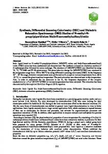
In Figure 5, we illustrate the experimental results and the results from this model for the melting of an 11.4 mg sample of water at different heating rates β . The exchange coefficients are adjusted for one rate; however, given the high value of these coefficients (as revealed by 4

1 2 3 4 5 6 7 8 9 10

previously published studies, e.g., [24]), parietal transfers are primarily limited by the phase change kinetics inside the sample, and erroneous values for these coefficients therefore does not significantly influence the final result. In Figure 5, we can observe that the melting “peak” becomes increasingly broad, on a Tplt scale, as the heating rate β increases, although, in accordance with the laws of thermodynamics, the enthalpy function has the same form for each experiment and depends only on the local temperature of the sample in each case. Thus, the melting of solid water begins and ends strictly at 0°C, despite the fact that the thermogram appears to show that this melting concludes at a positive temperature. In the paragraphs below, we will analyse the fact that the width of the peak increases as the heating rate increases.

11 12 13 14 15 16 17

If we attempt to employ the traditional method of “equivalent capacity”, which consists of deducing the enthalpy by integrating the thermogram as a function of the temperature of the plate (which is determined by time), the deduced “apparent enthalpy” function obtained from the experiment at β = 2 K/min is shown in Figure 6. This “apparent enthalpy” does not have the correct shape with respect to temperature, which should feature a sharp transition at the melting point, but it instead appears to be spread over a temperature range DTF; this range corresponds to the width of the thermogram.

18 19 20

It is noteworthy that if one uses the “apparent enthalpy” function in (9), instead of the formula that is provided in (10), a new thermogram is obtained that completely differs from the previous thermogram (see Figure 7).

21 22 23 24 25 26 27 28 29 30 31 32 33 34 35

In accordance with the model predictions and the experimental results (see Figure 5), DTF depends on the heating rate and the mass of the sample; this dependence is nonsensical, given that the phase change corresponds to a thermodynamic equilibrium. Because DTF, the width of the curve, decreases as the heating rate is reduced, the DTF-related issues could be minimised through the use of very low heating rates; however, overly low heating rates could cause the heat flows to be measured to become smaller than the detection threshold, which is determined by the noise that is present in the experiment. For calorimeters that use larger samples, the thermogram is always spread over several degrees of temperature, even if low heating rates are used. For instance, Figure 8 depicts the values of DTF at different heating rates for two different samples. The first sample has a mass of 8.5 mg, which corresponds to the mass that we use with our Pyris Diamond Perkin Elmer calorimeter cells, whereas the second sample has a mass of 78.3 mg, which corresponds to the mass used in the cells of other calorimeters (for example, Setaram) that are able to heat at lower rates. This figure indicates that the values of DTF depend on both mass and heating rate. They depend on the calorimeter used but in no case DTF can be cancelled.

36 37 38 39 40 41 42 43

The above analysis provides clear evidence that the shape of a thermogram is not a true representation of the derivative of the enthalpy with respect to temperature but is instead the result of complex heat transfers that occur during phase transforms. Our reasoning clearly applies to pure substances that completely melt at a constant temperature; however, similar results are observed for binary solutions [26] [Poitiers]. For example, Figure 9 presents the thermogram of the melting of a binary solution (which is characterised by eutectic melting followed by progressive melting), and Figure 10 illustrates the comparison between the “apparent enthalpy” (dashed line) and the true enthalpy (solid line).

44 45 46

As illustrated by Figures 6 and 10, we can observe that the inaccurate determination of the enthalpy by the method of “equivalent capacity” always produces an overly high estimate of the temperature range over which a phase transformation will occur.

47 5

1 2

3. The consequence of an incorrect enthalpy profile on the thermal performances of a wall that contains a PCM

3 4 5 6 7 8

In this study, to analyse the consequences of an inaccurate determination of the thermophysical properties of a PCM, we present a very simplified examination of a wall (see Figure 11) that is constructed from a composite containing a PCM (e.g., encapsulated PCM mixed with concrete). We will assess the one-dimensional case. Initially, we will assume that the wall and the outside (to the left of the wall) and inside (to the right of the wall) areas on each side of the wall are all at the initial temperature Tinit .

9 10

At time t = 0, a thermal solicitation Text ( t ) is applied to the left of the wall (at x = 0). Two cases are considered:

11 12

- First, a progressive heating from Tinit to Tmax that is regulated by an exponential function with a time constant τ :

⎡ ⎛ t ⎞⎤ Text ( t ) = Tinit + (Tmax − Tinit ) ⎢1 − exp ⎜ − ⎟ ⎥ ⎝ τ ⎠⎦ ⎣

13 14 15

(12)

- Second, a periodic function that could, for instance, simulates the changes in outdoor temperature that occur during the day-night cycle:

Text ( t ) = Text − ΔText ∗ cos ( 2π t / Ω )

16

(13)

17 18 19

where Text is the average temperature that is applied, ΔText is the amplitude of this solicitation, and Ω is the period of the function (in this instance, Ω =24 h). To avoid a sharp variation at t =0, we have chosen ΔText = Text − Tinit .

20 21 22

In the wall, the only heat transfer mode is conduction; consequently, the equation that must be solved is the same type of equation as (9). In one dimension, this equation may be written as follows:

∂ρ h ∂ 2T =λ 2 ∂t ∂x

23

(14)

24 25

The wall will be assumed to be a homogeneous PCM, but its latent heat will differ from l , the latent heat of the pure PCM, to reflect the mass fraction P < 1 of the PCM in the

26 27 28

concrete. Thus, l F = P l 0F . The values of thermal conductivity and heat capacity are linear interpolations (that depend on P ) from the corresponding values of pure concrete and pure PCM.

29 30 31 32 33 34 35

Two types of calculations will be considered. In the first calculation, we will use the correct enthalpy function (10) that is provided by the thermodynamic laws (the Heaviside function), whereas for the second calculation, we will use the apparent enthalpy. As explained above (see figure 9), several apparent enthalpies may be “constructed” from thermograms, depending on which sample masses and heating rates have been used for curve construction; in this study, we will characterise the different possible cases by DTF, the “deviation” of the enthalpy curve from the correct value (see Figure 6).

36 37

Our objective is to compare the results that are obtained for both of the cases that are described above. Thus, we will study the temperature profiles over time that are obtained at

0 F

6

1

several distances inside the wall and the values of the flux densities that enter (left) ϕ left and

2

leave (right) ϕ right the wall:

3

ϕ left = α (T ( 0, t ) − Text ( t ) )

(15)

4

ϕ right = α (T ( L, t ) − Tinit )

(16)

5 6 7 8

The chosen PCM (octadecane) has a melting temperature TF = 28 °C. We will assume that the wall contains P = 30% of a PCM; thus, for our calculations, we used l F = 72 kJ/kg, c S = c L = 1690 J/K.kg, ρ = 1385 kg/m3, λ = 0.65 W/m.K and α = 50 W/m2.K. The wall thickness is assumed to be L = 200 mm.

9 10

3.1 The case of exponential heating

11 12 13 14

We investigate the case of exponential heating that is described by equation (12), using the parameters of Tinit = 20 °C, Tmax = 50 °C and τ = 5 h. The results are given on Figures 12-14.

15 16 17 18 19 20

In Figure 12, we present the function Text ( t ) , the temperature at the left side of the wall and the results of the temperature inside the wall at x = 40 mm. We can demonstrate the effect of the PCM on the thermal behaviour of the wall, if we compare the curve for DTF = 0 K, which corresponds to the correct calculation that uses formulation (10) and the curve where no PCM exists in the wall ( l F = 0). The other curves on Figure 12 correspond to the results from apparent enthalpy calculations that use a DTF of 2, 5 or 10 K.

21

In Figures 13 and 14, we present the same comparison for the flux densities ϕ left and

22 23

ϕ right (the flux densities that enter the left side of the wall and leave the right side of the wall, respectively).

24 25

3.2 The case of periodic heating

26 27 28 29 30

We can also investigate the case of periodic heating, as specified in equation (13), using the parameters of Tinit = 20 °C, Text = TF = 28 °C, an amplitude of ΔText = Text − Tinit = 8 K and a period Ω = 24 h. We assume that there is no supercooling if the temperature is lower than the melting temperature. The results are given on Figures 15-17.

31 32

In Figure 15, we have presented the results for the function Text ( t ) , the temperature at the left side of the wall and the results of the temperature inside the wall at x = 40 mm.

33 34 35 36 37

Similarly to the case that was discussed in subsection 3.1, to address this situation, we present, in Figure 15, calculations to reveal the effect of the PCM by comparison between the curve for DTF = 0 K, which corresponds to the correct calculation that uses formulation (10) and the curve where no PCM exists in the wall ( l F = 0). The other curves on Figure 15 correspond to the results from apparent enthalpy calculations that use a DTF of 2, 5 or 10 K. 7

1

In Figures 16 and 17, we present the same comparison for the flux densities ϕ left and

2 3

ϕ right . (the flux densities that enter the left side of the wall and leave the right side of the wall, respectively).

4 5

3.3 Analysis of the results

6 7 8 9

First, in Figures 12- and 15, we observe the impact of the presence of the PCM in the wall and the real utility of PCMs, particularly for the stabilisation of temperature inside the wall and for lowering the levels of thermal flow that are exchanged at the right side of the wall.

10 11 12 13 14 15 16

In this paper, we do not intend to extend this analysis to a more complete study that examines different parameters, such as the nature of the PCM, its melting temperature, its concentration, the latent heat of the wall, the width of the wall and the initial levels of the various temperatures, among other factors. We are aware that this study only addresses very specific situations; however, the objective of the paper was to compare, for a given case, the effects of the “errors” that can be produced by inappropriate interpretations of the DSC thermograms.

17 18 19 20 21

If we examine the results that were obtained for the correct and the “apparent” enthalpies (Figures 12-14 and Figures 15-17), large differences are clearly evident between the correct approach and the calculations that rely on “apparent” enthalpies. As expected, these differences are larger for higher DTF values; from Figure 6, we can postulate that DTF values of 5 or 10 K are frequently obtained for reasonable DSC heating rates.

22 23 24 25 26 27 28

With regard to the temperature (Figures 12 and 15), we observed a difference of several degrees between the “apparent” enthalpy calculations and the exact result. We note that this difference inside the wall may be anecdotal, but the physics of heat transfer within the wall is not well represented. However, data regarding temperatures within a wall are vital; for instance, it is important to know which areas of a wall are actually affected by a phase transformation (as regions that are not affected by this transformation do not require the placement of a PCM).

29 30

With respect to heat flow densities, the differences between the two types of approaches are more evident for the incoming flux ϕ left than for the outgoing flux ϕ right .

31 32 33 34

For the exponential heating situation (Figures 13 and 14), we observe a difference between the two methods of up to 17% for ϕ left and a delay of a maximum of 2.8 h, whereas for ϕ right , we observe a difference of up to 35% after 20 h. These differences are considerable and reveal the necessity for accurate determinations of enthalpy.

35 36

For the periodic heating situation (Figures 16 and 17), we observe even greater differences between the results of the two methods; in particular, for ϕ left , a maximum difference of 43%

37

is observed, whereas for ϕ right , the difference can be as high as 25%. Moreover, we observe

38 39 40 41 42

that the maximum value of ϕ right is achieved up to 4.4 h after the time of the maximum predicted by the correct approaches. In this situation, we observe considerable differences between the two approaches, indicating that the knowledge of the temperatures and the exchanged energies in a system involving a PCM cannot be understood without determining the exact enthalpy, which illustrates the true changes of state that occur.

43 8

1

4. Conclusion

2 3 4 5 6 7 8 9 10

We have demonstrated that dynamic calorimetry, which is the preferred experimental technique for the energetic characterisation of a PCM, does not directly provide a specific enthalpy function with respect to temperature. Moreover, this study indicated that the “classical” method for the determination of enthalpies of a PCM through the simple integration of the experimental thermograms can produce very large errors if used for the determination of temperature fields or exchanged power in a wall that contains a PCM. In the case of thermal buildings, these thermal powers are directly related to energy consumption; in addition, the benefits of a more accurate determination of the energetic characteristics of any PCM are clearly evident.

11 12 13 14 15 16 17 18 19

In this investigation, we are aware that we have presented an academic case of a pure PCM. In this case, assuming that we could actually utilise a pure substance, it would be simple to determine, even by calorimetry, the melting temperature (onset) and latent heat (area of the thermogram) for the substance in question. The enthalpy function would then be completely determined. However, this determination is not the typical analytical procedure, even for pure substances. Thus, the aim of this article is to explain why the direct analysis of a calorimetry experiment inherently incorporates inaccuracies. Moreover, the case of unknown samples (solutions, composites, and other substances) could not be correctly treated in the typical manner.

20 21 22 23 24

Certain authors (see for example [27-30]) have suggested to determine h (T ) by the Thistory (or step) method. These experiments are very time consuming and certainly unsuitable for the very pure PCM. This is why we have chosen to characterise the PCM properties by inverse approaches of identification. This method has been satisfactorily validated for pure substances or aqueous saline solutions [31-33].

25 26

Acknowledgements

27 28 29

The three laboratories concerned by this study are funded by the MICPCM 2010 project of the ANR-Stock E program of the French National Research Agency

9

1

References

2 3 4

[1] Nomura T., Okinaka N., Akiyama T., Waste heat transportation system using phase change material (PCM) from steelworks to chemical plant, Resources, Conservation and Recycling 54 (2010) 1000–1006

5 6

[2] Kauffeld M., Wang M.J., Goldstein V., Kasza K.E. Ice slurry applications Review Article, International Journal of Refrigeration, Volume 33, Issue 8, December 2010, Pages 1491-1505

7 8

[3] Liu M., Saman W., Bruno F., Development of a novel refrigeration system for refrigerated trucks incorporating phase change material, Applied Energy, Volume 92, April 2012, Pages 336-342

9 10 11

[4] Pandiyarajan V., Chinnappandian M., Raghavan V., Velraj R. Second law analysis of a diesel engine waste heat recovery with a combined sensible and latent heat storage system, Energy Policy, Volume 39, Issue 10, October 2011, Pages 6011-6020

12 13

[5] Tan F.L., Tso C.P., Cooling of mobile electronic devices using phase change materials,Applied Thermal Engineering 24 (2004) 159–169.

14 15 16

[6] Wang Yi-Hsien, Yang Yue-Tzu, Three-dimensional transient cooling simulations of a portable electronic device using PCM (phase change materials) in multi-fin heat sink Original Research Article,Energy, Volume 36, Issue 8, August 2011, Pages 5214-5224

17 18

[7] Hammou Z.A., Lacroix M., A new PCM storage system for managing simultaneously solar and electric power, Energy and Buildings 38 (2005), 258–265.

19 20

[8] Huang M.J. The effect of using two PCMs on the thermal regulation performance of BIPV systems, Solar Energy Materials and Solar Cells, Volume 95, Issue 3, March 2011, Pages 957-963

21 22 23

[9] Chidambaram L.A., Ramana A.S., Kamaraj G., Velraj R., Review of solar cooling methods and thermal storage options Review Article, Renewable and Sustainable Energy Reviews, Volume 15, Issue 6, August 2011, Pages 3220-3228

24 25 26

[10] Chen Z., Gu M., Peng D. Heat transfer performance analysis of a solar flat-plate collector with an integrated metal foam porous structure filled with paraffin,Applied Thermal Engineering, Volume 30, Issues 14–15, October 2010, Pages 1967-1973

27 28

[11] Tyagi V.V., Buddhi D. PCM thermal storage in buildings: A state of art Review, Renewable and Sustainable Energy Reviews, Volume 11, Issue 6, August 2007, Pages 1146-1166

29 30 31

[12] Cabeza L.F., Castell A., Barreneche C., de Gracia A., Fernández A.I. Materials used as PCM in thermal energy storage in buildings: A review, Renewable and Sustainable Energy Reviews, Volume 15, Issue 3, April 2011, Pages 1675-1695

32 33

[13] Antony V. , Raj A., Velraj R. Review on free cooling of buildings using phase change materials, Renewable and Sustainable Energy Reviews, Volume 14, Issue 9, December 2010, Pages 2819-2829

34 35

[14] Kuznik F., David D., Johannes K., Roux J-J., A review on phase change materials integrated in building walls, Renewable and Sustainable Energy Reviews 15, 2011, Pages 379–391

36 37

[15] Heim D., Clarke J.A., Numerical modelling and thermal simulation of PCM–gypsum composites with ESP-r, Energy and Buildings, 2004, Volume 36, Pages 795–805

10

1 2

[16] Kuznik F., Virgone J., Noel J., Optimization of a phase change material wallboard for building use, Applied Thermal Engineering, Volume 28, Issues 11–12, 2008, Pages 1291-1298

3 4 5

[17] Koschenz M., Lehmann B., Development of a thermally activated ceiling panel with PCM for application in lightweight and retrofitted buildings, Energy and Buildings, Volume 36, Issue 6, June 2004, Pages 567-578

6 7 8

[18] Ibáñez M., Lázaro A., Zalba B., Cabeza L. F., An approach to the simulation of PCMs in building applications using TRNSYS, Applied Thermal Engineering, Volume 25, Issues 11–12, August 2005, Pages 1796-1807

9 10 11

[19] Kuznik F., Virgone J., Johannes K., Development and validation of a new TRNSYS type for the simulation of external building walls containing PCM, Energy and Buildings, Volume 42, Issue 7, July 2010, Pages 1004-1009

12 13 14

[20] Mazo J., Delgado M., Marin J.M., Zalba B., Modeling a radiant floor system with Phase Change Material (PCM) integrated into a building simulation tool: Analysis of a case study of a floor heating system coupled to a heat pump, Energy and Buildings, Volume 47, April 2012, Pages 458-466

15 16 17

[21] Günther E., Hiebler S., Mehling H., Redlich R., Enthalpy of Phase Change Materials as a Function of Temperature: Required Accuracy and Suitable Measurement Methods, International Journal of Thermophysics, 2009, Volume 30, Number 4, 1257-1269

18 19 20 21

[22] Castellón C., Günther E., Mehling H., Hiebler S., Cabeza L. F., Determination of the enthalpy of PCM as a function of temperature using a heat-flux DSC—A study of different measurement procedures and their accuracy, International Journal of Energy Research, 2008, Volume 32, Issue 13, pages 1258–1265

22 23 24

[23] He B., Martin V., Setterwall F., Phase transition temperature ranges and storage density of paraffin wax phase change materials, Energy, Volume 29, Issue 11, September 2004, Pages 1785– 1804

25 26 27

[24] Lazaro, A., Peñalosa, C., Solé, A., Diarce, G., Haussmann, T., Fois, M., Zalba, B., Gshwander S., Cabeza, L.F., Intercomparative tests on phase change materials characterisation with differential scanning calorimeter, Applied Energy, (2012) in Press

28 29

[25] Kousksou T., Jamil A., Zeraouli Y., Dumas J.P., DSC study and computer modelling of the melting process in ice slurry, Thermochimica Acta, 448 (2006), 123-129

30 31 32

[26] Zalba B., Marin J.M., Cabeza L. F., Mehling H., Review of thermal energy storage with phase change materials, heat transfer analysis and applications, Applied Thermal Engineering 23 (2003) 251283

33 34 35

[27] Zhang YP, Jiang Y, Jiang Y, A simple method, T-history method, of determining the heat of fusion, specific heat and thermal conductivity of PCM, Measurement Science Technology, 10 (1999), 3, 201-205

36 37 38

[28] Barreneche C., Solé A., Miró L., Martorell, I., Fernández A.I., Cabeza L.F., Study on differential scanning calorimetry analysis with two operation modes and organic and inorganic phase change material (PCM) Thermochimica Acta,553 (2013) 23-26

11

1 2 3

[29] Stankovic´ SB, Kyriacou PA. Improved measurement technique for the characterization of organic and inorganic phase change materials using the T-history method. Appl Energy (2013) (in press),

4 5 6

[30] Lin W., Dalmazzone D., Fürst W., Delahaye A., Fournaison L., Clain P., Accurate DSC measurement of the phase transition temperature in the TBPB–water system, J. Chem. Thermodynamics 61 (2013) 132–137

7 8 9

[31] Gibout S., Franquet E., Dumas J.P., Bédécarrats J.P. Détermination de l’enthalpie de fusion de solutions par une méthode inverse à partir d’expériences simulées de calorimétrie, Congrès SFT Perpignan 24-27 Mai 2011

10 11 12 13

[32] Gibout S., Maréchal W., Franquet E., Bédécarrats J.P, Haillot D. Dumas J.P., Determination of the enthalpy of phase change materials by inverse method from calorimetric experiments. Applications to pure substances or binary solutions. 6th European Thermal Sciences Conference Eurotherm 12, Poitiers-Futuroscope 4-7th September 2012

14 15 16

[33] Franquet E., Gibout S., Bédécarrats J.P., Haillot D., Dumas J.P., Inverse method for the identification of the enthalpy of phase change materials from calorimetry experiments, Thermochimica Acta 546 (2012) 61– 80

17

12

1 2 3 4

Figures captions Fig. 1. Melting thermograms for water at 2 and 5 K/min (green and red curves, respectively) and the derivative of the observed enthalpy (blue curve).

5 6

Fig. 2. Melting thermograms for a 3% aqueous solution of NH4Cl at 2 and 5 K/min (green and red curves, respectively) and the derivative of the observed enthalpy (blue curve).

7

Fig. 3. Scheme of the DSC head (Pyris Diamond Perkin Elmer).

8

Fig. 4. A model of a DSC cell.

9

Fig. 5. Thermograms for the melting of water at different heating rates.

10 11

Fig. 6. A comparison of the “apparent enthalpy” function that is obtained via the “equivalent capacity” method (red) and the true enthalpy function (blue) for water.

12 13

Fig. 7. The numerical thermograms that are obtained from the apparent enthalpy (red) and the true enthalpy (blue).

14

Fig. 8. The DTF versus β (which is measured on a logarithmic scale) for two sample masses.

15 16

Fig. 9. The experimental thermogram of a 9.02% H2O/NH4Cl binary solution that is heated at 5 K min-1

17

Fig. 10. The “apparent” (dashed) and exact (solid) enthalpy curve for the binary solution

18

Fig. 11. A schematic view of a wall that contains a PCM.

19 20 21

Fig. 12. The imposed temperature Text ( t ) and the temperature at x = 40 mm, as calculated by the correct method (DTF = 0) and by different incorrect analyses of the thermogram with DTF = 2, 5 or 10 K

22 23 24

Fig. 13. The flux densities ϕ left that enter at the left side of the wall, as calculated by the correct method (DTF = 0) and by different incorrect analyses of the thermogram with DTF = 2, 5 or 10 K

25 26 27

Fig. 14. The flux densities ϕ right that leave the right side of the wall, as calculated by the correct method (DTF = 0) and by different incorrect analyses of the thermogram with DTF = 2, 5 or 10 K

28

Fig. 15. The imposed temperature Text ( t ) and the temperature at x = 40 mm, as calculated by the correct method (DTF = 0) and by different incorrect analyses of the thermogram with DTF = 2, 5 or 10 K

29 30 31 32 33

Fig. 16. The flux densities ϕ left that enter the left side of the wall, as calculated by the correct method (DTF = 0) and by different incorrect analyses of the thermogram with DTF = 2, 5 or 10 K

13

1 2 3

Fig. 17. The flux densities ϕ right that leave the right side of the wall, as calculated by the correct method (DTF = 0) and by different incorrect analyses of the thermogram with DTF = 2, 5 or 10 K

4 5

14

1 2 3 4 5 6

Figure 1

15

1 2 3 4 5

Figure 2

16

1 2 3 4 5

Figure 3

17

1 2 3 4

Figure 4

18

120

2D cylindrical model Experiment

10K/min

60 5K/min

[mW ]

80

15K/min

100

2K/min

40

20

0 0

5

10

15

20

T [ C] 1 2 3 Figure 5 4Figure 8: Comparison of the experimental thermograms with the numerical thermograms

obtained with a 2D cylindrical model.

12

19

1 2 3 4

Figure 6

20

1 2 3 4

Figure 7

21

1 2 3 4

Figure 8

22

1 2 3 4

Figure 9 and Figure 10

23

1 2 3 4

Figure 11

24

1 2 3

Figure 12

25

1 2 3 4

Figure 13

26

1 2 3 4

Figure 14

27

1 2 3 4

Figure 15

28

1 2 3 4

Figure 16

29

1 2 3

Figure 17

30