Correlated Component Regression - Statistical Innovations

(Reprinted from the 2010 American Statistical Association Proceedings with Edits)

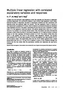
Correlated Component Regression: A Prediction/Classification Methodology for Possibly Many Features Jay Magidson Statistical Innovations Inc., 375 Concord Ave., Ste. 007, Belmont, MA 02478

Abstract A new ensemble dimension reduction regression technique, called Correlated Component Regression (CCR), is proposed that predicts the dependent variable based on K correlated components. For K = 1, CCR is equivalent to the corresponding Naïve Bayes solution, and for K = P, CCR is equivalent to traditional regression with P predictors. An optional step-down variable selection procedure provides a sparse solution, with each component defined as a linear combination of only P* < P predictors. For high-dimensional data, simulation results suggest that good prediction is generally attainable for K = 3 or 4 regardless of the number of predictors, and estimation is fast. When predictors include one or more suppressor variables, common with gene expression data, simulations based on linear regression, logistic regression and discriminant analysis suggest that CCR predicts outside the sample better than comparable approaches based on stepwise regression, penalized regression and/or PLS regression. A major reason for the improvement is that the CCR/step-down algorithm is much better than other sparse techniques in capturing important suppressor variables among the final predictors.

Keywords: High dimensional data; variable reduction; correlated component regression; naïve Bayes; suppressor variable; penalized regression

Keywords: High dimensional data, variable reduction, correlated component regression, 1. Background and Introduction When the number of predictor variables P approaches or exceeds the sample size N (high dimensional data), coefficients estimated using traditional regression techniques become unstable or cannot be uniquely estimated due to multicolinearity (singularity of the covariance matrix), and logistic regression has an additional problem, providing complete or quasi-complete separation in the analysis sample. However, seemingly good performance in the analysis sample is often due to overfitting, and does not generalize as well as certain kinds of restricted models to new cases outside the sample. Approaches for developing restricted models that yield regularized solutions include a) penalized regression methods such as Lasso and Elastic Net, which impose explicit penalties referred to as L1 or an average of L1 and L2 regularization respectively, and b)

1

dimension reduction approaches such as Principle Component Regression (PCR) and PLS Regression, which reduce the dimension of the problem to K < min (P, N-1), and Naïve Bayes which reduces the dimension to 1. Generally speaking, with high dimensional data, a substantial amount of regularization may be needed, via small values for K, to obtain reliable results. In this paper, we describe an alternative dimension reduction approach called Correlated Component Regression (CCR) and an associated step-down algorithm for reducing the number of predictors in the model to P* < P. Similar to traditional regression, CCR has different variants depending upon the scale type of the dependent variable. Regardless of the scale type, the saturated CCR model, which occurs when K  Ksat = min (P, N-1)1, is equivalent to the corresponding traditional regression model (e.g., linear regression, logistic regression, linear discriminant analysis). As explained in section 3.1, use of Ksat components does not involve any reduction in dimensionality, and hence produces predictions equivalent to traditional regression. When the outcome is categorical, the 1-component CCR model is equivalent to Naïve Bayes classification. More generally, for any scale type, the 1-component CCR model may be viewed as a natural generalization of Naïve Bayes, the key being to represent the Naïve Bayes conditional independence assumption in a discriminative as opposed to generative form. For the distinction between these different model forms, see Ng and Jordan (2002) and Mitchell, 2005. We further suggest that for K > 1, CCR represents a natural extension of Naïve Bayes to multiple dimensions. A hybrid version of CCR is also proposed that involves mixed predictor scale types. For example, in the case of a dichotomous dependent variable, when both continuous and categorical predictors are present, the coefficients for the continuous predictors can be estimated according to variant CCR-LDA (if the normality assumptions in linear discriminant analysis are appropriate), while those for the categorical predictors are estimated according to CCR-Logistic, which imposes no distributional assumptions on the predictors. Results from simulations and applications with real high dimensional data suggest that CCR models rarely require more than 10 components regardless of the number of predictors, and usually perform well with 3 or 4 components. With such a small number of components estimation is fast, which allows employment of M-fold cross-validation to determine the optimal values for the tuning parameters K and P. This paper is organized as follows: Section 2 illustrates the general high dimensional data problem with the application of a stepwise logistic regression analysis to a small sample of cases from real data where P > N. Section 3 discusses some sparse and non-sparse regression approaches that have been proposed for use with high dimensional data. Section 4 introduces the general CCR approach and section 5 summarizes some simulation results. Section 6 compares results of more detailed analyses of the data described in Section 2. 1

Saturation may also occur prior to min(P, N-1) components.

2

2. Logistic Regression with More Features than Cases: P > N The logistic regression model for dichotomous dependent variable Z and P predictors is: P

Logit (Z )      g X g g 1

• • •

As P approaches the sample size N, overfitting tends to dominate and estimates for the regression coefficients become unstable Complete separation between the groups Z=1 and Z=0 is always attainable for P =N-1 Traditional algorithms do not yield unique coefficient estimates when P ≥ N as coefficients are not identifiable

Table 1 and Figure 1 present results of applying the forward stepwise logistic regression option in the SPSS logistic regression procedure to a dataset with a dichotomous dependent variable, N = 40 cases and P = 85 dichotomous predictors. The p-value to enter the model was set to .999. An additional N=360 cases are retained for model validation. More specifics of the data and design are given in section 6. Table 1 shows that beginning in step 5 when perfect separation is achieved with 5 predictors (AUC = 1 in the training data plot shown in Figure 1), the coefficients and standard errors become extremely large in magnitude and the associated coefficients no longer are statistically significant. This is indicative of the effects of multicolinearity. Despite the fact that these coefficient estimates are not (uniquely) identifiable, they can still be used to score the training and validation data. The plot of the validation results in Figure 1 show that a decline from AUC=.8 also begins to occur in this 5th step. This result is consistent with the hypothesis that prediction deteriorates due to overfitting when more than 4 predictors are included in the model.

Table 1: Results from Stepwise Logistic Regression Estimated on Training Data

3

Variables in the Equation Coef. std. err. p-value Step 1(a) item31e -2.8 0.8 0.00058 Constant 4.3 1.4 0.0019 Step 2(b) item31e -3.5 1.1 0.0024 item55e -2.6 1.1 0.022 Constant 9.0 3.1 0.0037 Step 3(c) item31e -3.9 1.3 0.0023 item55e -3.3 1.3 0.012 item20j 2.6 1.1 0.021 Constant 7.0 3.2 0.028 Step 4(d) item13e 3.4 1.6 0.038 item31e -4.3 1.6 0.007 item55e -4.3 1.7 0.014 item20j 3.3 1.4 0.018 Constant 3.8 3.8 0.31 Step 5(e) item13e 66.5 6919.5 0.99 item31e -99.8 9559.0 0.99 item55e -115.6 11089.9 0.99 item1j 82.0 7970.4 0.99 item20j 66.5 6898.5 0.99 Constant 17.2 7017.9 1.00 Step 6(f) item13e 69.5 9523.3 0.99 item26e -37.8 11949.3 1.00 item31e -68.0 8272.2 0.99 item55e -101.9 11276.6 0.99 item1j 67.3 8183.0 0.99 item20j 33.7 5459.6 1.00 Constant 54.9 16806.2 1.00

4

Figure 1: Results from Stepwise Logistic Regression Estimated on Training Sample 3. Some Sparse and Non-sparse Approaches to Logistic Regression Since perfect discrimination is achieved with only 5 predictors in our example above, this raises the possibility that to achieve the best predictions no more than 4 or 5 predictors should be included in the model. The 5-predictor solution is said to be sparse because the coefficients for each of the remaining 80 predictors are set to 0. Stepwise regression is the most widely used technique to obtain a sparse regression solution. Alternative approaches include sparse component approaches and sparse penalized regression methods. In addition, non-sparse regression approaches such as ridge regression are also available to control how large the coefficients and standard errors can become as P increases and to achieve reliable prediction with P>N in the case of high dimensional data. Below we summarize the major (sparse and non-sparse) component approaches and provide references to some sparse penalized regression approaches that have been proposed.

3.1 Component approaches a) Principal Component Regression (PCR) – PCR transform the predictors X1, X2, …, XP to principal components, S1, S2, …, SP, each component defined as a weighted sum of all the predictors. Then, the first K < P components (those explaining the most predictor variance) are used as predictors in the model. Advantages over stepwise regression are: 1) PCR takes into account information on more predictors. While there are only K < P predictors in model, each component incorporates information on all the X variables, thus possibly providing better prediction of Z.

5

2) Since components are multicolinearity go away.

orthogonal

(uncorrelated),

problems

due

to

Disadvantages of PCR are: 1) To apply the model, one needs measurements of all P of the X variables. 2) One or more of the components might not be predictive of the dependent variable Z, and the resulting model might not predict better than that obtained by stepwise regression. 3) The components are not as interpretable. Regarding interpretability (disadvantage #3), since each component is a weighted sum of the Xs, substituting for the components, one gets coefficients for the Xs. For example, for K = 2 components, we have: P

S1    g .1 X g g 1

which yields:

P

S 2    g .2 X g

Logit (Z )    b1.2 S1  b2.1S 2

g 1

P

Logit (Z )     (b1.2  g .1  b2.1 g .2 ) X g g 1

From this latter equation we see that the effect for each predictor can be decomposed into separate effects (loadings) associated with each component. Thus, if the components were more meaningful, the coefficients of the Xs will also be more meaningful. In particular, we will see that the CCR components are more meaningful – the loadings on component 1 correspond to direct effects and the loadings on component 2, which frequently has a moderate to high correlation with component 1, capture indirect effects. In particular, pure suppressor variables have zero loadings on component 1 but highly significant loadings on CCR component #2. Magidson and Wassmann (2010) argue that suppressor variables are often among the most important predictors in a model. b) Supervised PCR (SPCR). Regarding predictability (PCR disadvantage #2), a modified version of PCR called Supervised PCR (SPCR: Bair, et. al., 2006) has been proposed. Rather than using the first K components as the predictors in the model, SPCR selects only the K components that are significant predictors of Z. The obvious advantage of SPCR over PCR is that each component is assured to be predictive (individually) of Z. An important disadvantage however is that it tends to exclude components that act as suppressor variables. As such, when one or more suppressor variables are included among the P predictors, SPCR may provide poorer prediction than PCR. c) PLS regression. PLS regression differs from PCR and SPCR in that the dependent variable is utilized in addition to the predictors in forming the K components. As a result, it will generally contain fewer components and be more predictive than PCR and SPCR. However, similar to PCR and SPCR, the components are orthogonal, which means that they are not as interpretable as those obtained in CCR and when one or more suppressor variable exists among the P predictors, more components are required to capture the suppressor variable effects than CCR. An additional disadvantage of each of these approaches is that they are non-sparse. That is, to apply the model to new data, one needs measurements on all P of the X variables.

6

d) Sparse PLS regression. SPLS (Chun and Keles, 2009) is a modified version of PLS regression that also includes variable reduction. A disadvantage is that when one or more suppressor variables is included among the P predictors, our simulation results (section 5) suggest SPLS does not predict as well as CCR, and is less likely to capture the suppressor variable(s) than if the CCR step/down algorithm is used for variable reduction. e) Naïve Bayes Consider first the situation with a dichotomous dependent variable, Z = 1 or 0. In this case the conditional probability of being in group 1 given the predictors X, denoted P(Z=1|X), may be predicted using the traditional logistic regression model, and if X follows the multivariate normal distribution with different group means but common variances and covariances within each group, efficient estimates for the coefficients can be obtained from LDA (Efron, 1975). Since Naïve Bayes (NB) is justified under the assumption that the predictors are conditionally independent given each outcome category, when the data follows the LDA assumptions, NB is equivalent to LDA performed with a diagonal variance covariance matrix (Ng, A. and M. Jordan, 2002). The coefficient estimate for a given predictor in the discriminative form of NB is thus equivalent to the usual estimate for the population logodds ratio, which takes the form ( 1  0 ) /  2 . This quantity is obtained by LDA with a single predictor, and thus is equivalent to the 1-component CCR-LDA model. Similarly, if we maintain the assumption of conditional independence but relax the LDA assumptions, the NB-type coefficients can be obtained from corresponding 1-predictor logistic regressions (see e.g., Mitchell, 2005), which is equivalent to the 1-component CCR-Logistic model.

3.2 Sparse Penalty Regression Approaches Unlike ridge regression which makes use of L2 regularization, use of L1- regularization results in sparse solutions; i.e., solutions where some of the regression coefficients equal 0. In this way, dimensionality is reduced. Since L1- regularization involves a convex loss function, its implementation is computationally efficient (Friedman, et. al, 2010). Recently, algorithms involving non-convex loss functions such as SCAD, and MCP have been proposed (see e.g., NCVREG R package). While both the (non-sparse) component methods and sparse penalized approaches both reduce the dimensionality to include only K < P predictors, they do so in very different ways. The component methods replace the predictors by fewer components, while the sparse penalty methods eliminate certain predictors by setting their coefficients to 0. The 3 sparse penalty approaches that are included in our simulation study are: a) LARS/Lasso (L1- regularization): GLMNET (R package) b) Elastic Net (Average of L1 and L2 regularization): Zou and Hastie (2005) GLMNET (R package) c) Non-convex penalty: e.g., TLP (Shen, et. al, 2010)

7

4. Correlated Component Regression 4.1 CCR General Description Correlated Component Regression (CCR) is a general approach for the development of a sequential K-component predictive model, each component estimated by application of the naïve Bayes rule to deal with the effects of multi-colinearity. In particular, with high dimensional data it has been shown that use of the Naïve Bayes Rule: “greatly outperforms the Fisher linear discriminant rule (LDA) under broad conditions when the number of variables grows faster than the number of observations”, Bickel and Levina (2004) even when the true model is that of LDA! In practice, Dudoit et al. (2002) found that naïve Bayes outperformed LDA in classifying tumors based on gene expression data. Results from simulated data (section 5) suggest that CCR outperforms other sparse regression methods, with generally good outside-the-sample prediction attainable with K=2, 3, or 4. In addition, several applications with gene expression data suggest that CCR may be quite useful in practice Magidson (2010). Magidson and Wassmann (2010) provide an application in the early detection of prostate cancer and suggest that an important reason for the good performance of CCR is that it is designed to capture the effects of suppressor variables when such are included among the predictors. Suppressor variables, called “proxy genes” in genomics (Magidson and Wassmann, 2010), have no direct effects, but improve prediction by enhancing the effects of genes that do have direct effects “prime genes”. Based on experience with gene expression and other high dimensional data, suppressor variables often turn out to be among the most important predictors:  9-gene model for prostate cancer (single most important gene, SP1, is a proxy gene (Magidson and Wassmann, 2010) 

Survival model for prostate cancer (3 prime and 3 proxy genes supported in blind validation), Magidson (2010)



Survival model for melanoma (2 proxy genes in 4-gene model supported in blind validation), Magidson (2010)

Despite the extensive literature documenting the strong enhancement effects of suppressor variables (e.g., Horst, 1941, Lynn, 2003, Friedman and Wall, 2005), most prescreening methods omit proxy genes prior to model development, resulting in suboptimal models. This is akin to “throwing out the baby with the bath water”. Because of their sizable correlations with associated prime genes, proxy genes can also provide structural information useful in assuring that these associated prime genes are selected with the proxy gene(s), improving over non-structural penalty approaches.

8

Just as there are several different variants of regression to deal with different assumptions associated with the distributions and scale types of the dependent variable and predictors, there are several variants of CCR – one for each different type of regression: CCR-Linear – Continuous dependent variable CCR-LDA – Dichotomous dependent and continuous predictors satisfying assumptions of linear discriminant analysis (LDA) CCR-Logistic – Dichotomous dependent variable CCR-Ord – Ordinal dependent variable CCR-Nom – Nominal dependent variable CCR-Cox – Survival analysis (right censored event history data) CCR-Latent – Dependent variable represented by latent classes In the remainder of this section we describe the general approach and illustrate it with equations pertaining to CCR-Logistic. In section 5 we summarize simulation results associated with the first 2 variants above and section 6 presents new results from real data on the CCR-Logistic variant. For further details on CCR-LDA, CCR-Ord and CCR-Nom see Magidson (2010).

4.2 CCR General Algorithm Correlated Component Regression (CCR) utilizes K correlated components, each a linear combination of the predictors X1, X2, …, XP, to predict an outcome variable Z. Step 1: The first component S1 captures the effects of prime predictors which have direct effects on the outcome. It is an average (ensemble) of all 1-predictor effects. For example, for CCR-Logistic: Form 1st component S1 as weighted average of P 1-predictor models (ignoring g) :

Logit ( Z )   g   g X g 1-component model:

g=1,2,…,P;

S1 

1 P  g X g P g 1

(1) (2)

Logit (Z )     S1

Step 2: The second component S2, correlated with S1, captures the effects of suppressor variables (proxy predictors) that improve prediction by removing extraneous variation from S1. For example, for CCR-Logistic: Step 2: Form 2nd component S2 as an average of the

 g .1 X g terms

 g .1 is estimated from the following P=2-predictor logit model: 1 P Logit ( Z )   .1   g S1   g .1 X g g=1,2,…,P; S 2    g .1 X g P g 1

where each

(3)

Step 3: Estimate the 2-component model using S1 and S2 as predictors:

Logit (Z )    b1.2 S1  b2.1S 2

(4)

Continue for K = 3,4,…,K*-component model. For example, for K=3, step 2 becomes:

Logit (Z )   .12   g .1S1   g .2 S2   g .12 X g 9

(5) The CCR-linear algorithm, which is the generalization of the CCR-logistic algorithm described above to the case of a continuous predictor Y is straightforward. Logit(Z) is simply replaced by Y in the above equations, an error term can be added at the end of the equations, and OLS is used to obtain the coefficient estimates. Step 3A: In the case of CCR-LDA, we can utilize the random X normality assumption to speed up the CCR-logistic algorithm, to be comparable to the speed of CCR-linear. For example, in the step for component K, regress each predictor on Z, controlling for S1,…,SK-1 in fast linear regressions: e.g., for K=1:

X g   g   g' Z

 g   g' / MSE

S1 

g=1,2,…,P;

1 P  g X g P g 1

(6) (7)

where g is the maximum likelihood estimate for the log-odds ratio in the simple logistic regression model (Lyles et al., 2009). Note that this approach also accomodates missing values on predictors, since cases missing on predictor Xg can simply be excluded from the regression in eq. (6). In addition, CCR-ord can be performed by simply replacing the dichotomous Z by the full ordinal dependent variable based on the sterotype ordinal regression (see e.g., Magidson 1996). Step 3B: Alternatively, in the case of CCR-LDA, in the step where we wish to estimate eq. 5 when K components have already been estimated (K=2 being illustrated in eq. 5), we assume that the attenuated vector S=(S1, S2, …,SK,Xg) is distributed according to MVN distribution with different group means but common covariances and estimate the LDA coefficients directly using the standard LDA formula. This is equally fast as step 3A, both 3A and 3B avoiding iterative algorithms (e.g., iteratively reweighted least squares) used to estimate the logistic regression model. Step 3C: A hybrid CCR approach can be used when the predictors are of mixed scale types. For example, suppose that X1 is dichotomous but X2 is continous. Since the predictors enter into the equations one at a time, we can use the approach that is most appropriate to estimate the log-odds ratio and partial log-odds ratio coefficients for each predictor. For example, at the step where 2 components have been estimated, we can estimate the coefficients for the components and for Xg in the logistic regression equation (5), we can use traditional logistic regression when g=1 to obtain the coefficient for X1 and use the LDA formula when g=2 to obtain the coefficient for X2. 4.3 Correlated Component Regression Step-down Variable Reduction Step Step SD: For a given K-component model, eliminate the variable that is the least important, where importance is quantified as the absolute value of the variable’s standardized coefficient, where the standardized coefficient is defined as:

 g*   g  g 10

(8)

For example, suppose we are evaluating models with K = 2, and that predictor g* is found to be least important, being the predictor that has the smallest absolute value of its standardized coefficient in the 2-component model. Then that predictor would be excluded and the steps of the CCR estimation algorithm repeated on the reduced set of predictors. In practice, in the case of large P, more than 1 predictor can be eliminated at a time. For example, at each step we can eliminate the 1% of the predictors that are least important until P < 100, at which time we can begin eliminating 1 predictor at a time. This process can continue until 1 predictor remains. Note that for P = K, the model becomes ‘saturated’ and is equivalent to the traditional regression model. In order to reduce the number of predictors further, we maintain the saturated model by reducing K so that P = K. Thus, for example, for K = 4, when we step down to 3 predictors, we reduce K so K = 3. Use of M-fold cross-validation is used to determine the optimal value for the tuning parameters K and P for a given criterion (or loss function). For computational efficiency, this is done first for K=1 components, then K=2 components, ... , up through say K=8 components. Since in practice, the optimal number of components will rarely be greater than 8, one can be fairly sure of obtaining a good model with K < 9. For a given number of components K, the optimal number of predictors P*(K), can then be determined, and (P*, K*) can be determined as the combination minimizing the loss function. Thus, P* predictors will be retained where P* is the best of the P*(K), K=1,..., 8, and K* will be the optimal number of components associated with P* predictors. Evaluating up to only 8 components saves computer resources since the speed of CCR increases exponentially as the number of components increases. Since estimation utilizes a sequential process, most of the sufficient statistics from previous runs can be reused. Hence, CCR is very fast with a small number of components. Let A(K) = cross-validated accuracy for the K-component model based on the optimal number of predictors P*(K). Then, if A(1) < A(2) < A(3) < A(4) > A(5), we might stop after evaluating K = 5 and not evaluate K=6,7,8, saving more computer time. That is, if the 5-component model fails to provide a solution that improves over the 4-component model according to the results of the M-fold cross-validation, we might take K* = 4, and P* = P*(4). As a somewhat more conservative approach, we might also evaluate K = 6 to check that performance continues to degrade. The use of M-fold cross-validation to determine the optimal value for one or more 'tuning parameters' is standard practice in data mining. It is used for example, to obtain the single tuning parameter 'lambda' in the lasso penalized regression approach. Here, we use it to optimize the two tuning parameters, P and K. We do it in an efficient way by doing it for each component separately, and evaluate only a small number of models (those with K in a specified range), and limit to small values of K. In practice with highdimensional data, we have found that the best model is rarely one with K>8.

11

For ultra-high dimensional data with many irrelevant predictors, typical with gene expression data, by chance some large loadings for the many irrelevant predictors may dominate the first component, leading to unreliable results. To avoid this, an initial variable selection ‘screening’ step may be performed to reduce # predictors to a manageable number prior to model estimation. Most current screening methods should be avoided because they typically exclude important suppressor variables. These include supervised principle components analysis/SPCA: (Bair, et. al., 2006), as well as the SIS approach (Fan and Lv, 2008). Fan and Lv (2008) distinguish between high and ultra-high dimensional data, and propose ISIS to pre-screen predictors in ultra-high dimensional data where suppressor variables may be present. Fan et. al. (2009) present ISIS simulation results based on 3 prime predictors and one suppressor variable which shows a large improvement over SIS. While promising, ISIS has been criticized for having too many tuning parameters. We are developing a CCR-based screening procedure, CCR/Screen, that has a single parameter P*, or the desired number of predictors to be selected (Magidson and Yuan, 2010). Section 5.3 shows that CCR/Screen outperforms ISIS on the simulation data provided in Fan. et. al (2008, 2009) that includes a suppressor variable. Our screening procedure is based on a restricted 3-component CCR model, developed as follows: For Component 1: Apply Inverse normal transformation to Comp. #1 p-vals > .5 to get Zval1, and use 2-class truncated normal mixture (latent class) model on -Zval1 to identify the G1 most significant predictors (G1 predictors whose posterior prob >.5 of being in class with lowest p-vals). Set component #1 loadings to 0 for all but G*1 predictors, where G*1 = min{max{ G1, 2}, 10}. For Component 2: Compute Zval2= Inverse normal of Comp #2 p-vals > .5 (excluding the G*1 predictors identified above), and estimate latent class model on -Zval2 to identify G2 predictors assigned to lowest component #2 p-val class. Set the loading to 0 for all but the G*2 predictors with lowest p-values (excluding the G*1 predictors), where G*2 = min{max{ G2, 1}, G1}. For Component 3: Set the loading to 0 for all but the M predictors with lowest p-values. introduce CCR/Select and compare its performance with ISIS based on Fan et. al. (2009) simulated data. See Magidson and Yuan (2010)

5. Simulation Results CCR, as implemented in the CORExpress™ program, is compared to alternative methods M=1,2,… across 3 different simulation studies (Magidson and Yuan, 2010). Some results from each of 3 different simulation studies are given below: 1) LDA: CCR-LDA vs. penalized regression and sparse PLS regression 2) Linear Regression: CCR-Linear vs: penalized regression 3) LDA Variable Screening – CCR-LDA/Select vs. ISIS

5.1 Simulation for CCR-LDA Here, data were simulated according to assumptions of Linear Discriminant Analysis.

12

P = G1 + G2 where G1 = 28 predictors (including 15 weak predictors) and G2 = 28 irrelevant predictors. 2 Groups: N1 = N2 = 25; 100 simulated samples. Method M selects G*(M) < 56 predictors for final model; Methods tuned using same sized validation file. Final models from each method evaluated based on large independent ‘test’ file. (In practice, M-fold cross-validation is used to optimize the CCR models when validation files are not available.) Variable selection METHODS: Correlated Component Regression (CCR), Elastic Net (L1 + L2 regularization, Zou and Hastie, 2005), Lasso (L1 regularization), and sparse PLS regression (sgpls, Chun and Keles, 2009) Results favor CCR over the other approaches Lowest misclassification error rate: CCR (17.4%), sparse PLS (19.1%), Elastic net (20.2%), lasso (20.8%) Fewest irrelevant variables: CCR (3.4), lasso (6.2), Elastic net (11.5), sparse PLS (13.1) Most likely to include suppressor variable SP1 (% of simulations): CCR (91%), sparse PLS (78%), Elastic Net (61%), lasso (51%) Average # predictors in model: lasso (13.6), CCR (14.5), Elastic Net (19.2), sparse PLS (20.4) Most sparse solution (average # predictors in model): CCR (14.5), lasso (17.3), Elastic net (28.3), sparse PLS (32.3)

5.2 Simulation for CCR-Linear Data were simulated according to assumptions of Linear Regression G1 = 14 predictors + G2 = 14 irrelevant predictors correlated with true predictors + G3 = 28 irrelevant predictors uncorrelated with true; Continuous dependent variable, N = 50, population R2 = 0.9; 100 simulated samples Method M selects G*(M) < 56 predictors for final model; Each method tuned using a validation file with N=50. Final models from each method evaluated based on large independent ‘test’ file. TLP = nonconvex (truncated L1) penalty (Shen, et. al., 2010) Again, results favor CCR over the other approaches: Number of ‘True’ Predictors included, Percentage of included that were ‘True’: CCR (9.7, 78%), TLP (10.3,50%), sparse PLS (9.5, 48%), Elastic Net (12, 35%) Fewest irrelevant uncorrelated variables: CCR (1.0, 8%), TLP (6.4, 31%), sparse PLS (6.4, 33%), Elastic Net (14.1, 41%) Fewest irrelevant correlated variables: CCR (1.8, 15%), sparse PLS (4.4, 22%), Elastic Net (8.0, 23%), TLP (4.0, 27%) Lowest mean squared error: CCR (3.13), sparse PLS (3.34), Elastic Net (3.50), TLP (3.55) # tuning parameters: CCR (3x50), sparse PLS (3x50), TLP (5x100), Elastic Net (10x50)

5.3 Simulation for Variable Screening 13

Here we simulated 100 data sets with 4 true predictors, the 4th being a suppressor variable. The data were simulated according to specifications of Fan et. al. (2009) with N=200: Logistic Regression with 0= 0, effects of primes 1 = 2 = 3 = 4; effect of suppressor =  4  6 2 and predictors X5 - X1000 are irrelevant: 5 = 6 = … = 1000 = 0. 1000

Logit ( Z )   0    g X g g 1

where X follows a multivariate normal distribution with means 0, variances 1 and all correlations = .5 except that corr ( X i , X 4 )  1 / 2 for i ≠ 4. CCR/Screen includes the suppressor variable X4 among the 10 top predictors 91% of the time compared to only 80% for ISIS. In addition, ISIS performed very poorly when fewer than 7 predictors were selected.

Figure 2: Simulation results showing the improvement of CCR/Screen over ISIS.

14

6. Case study: Logistic Regression on High Dimensional Data A small sample of N=40 cases (‘training data’, ‘analysis sample’) was selected from a larger sample of N=400, the remaining larger number of cases (“validation data”) being used to evaluate the predictive performance of the resulting high dimensional regression models. For further information on these data see Wyman and Magidson (2008). 6.1 Design of P > N Example with Real Meyers-Briggs (MBTI) Data •

Dependent variable Z is the dichotomous self validated Extraversion/Introversion scale: Z=1 for 220 Extraverts (E) , Z=0 for 180 Introverts (I)

• •

Total sample size: 400 cases with no missing on any of the 85 predictors randomly select 10% for training sample -- 22 E + 18 I = total N(TRAIN)= 40 N(VALIDATION) = 360 Use 85 dichotomous features – 84 items from MBTI Form G plus 1 item that is an Enneagram-3 identifier (see Wyman and Magidson, 2008 for the relationship between Enneagram-3 types and the EI dimension of MBTI).

•

Item Description

# items

20 EI items -21 JP items 20 SN items 23 TF items Enneagram-3

20 21 20 23 1

# significant in sample validation training 20 12 10 4 3 2 3 0 0 1

Table 2: Relationship between Self-validation and Classification based on EI items using MBTI Scoring The results in Table 2 are consistent with known misclassification rates. Theoretically, the E-I items should be the ones selected into the predictive model. However, Extraverts tend to be more likely to be Perceiving as opposed to Judging types than Introverts, and thus, some J-P items may also enter, as well as the Enneagram-3 indicator.

15

The inclusion of S-N and T-F items should be an indicator of over-fitting since these would be extraneous predictors.

6.2 Validation Sample Results Obtained from CCR/Step-down Algorithm

Figure 3: Results from the CCR Algorithms CCR selection Criterion: Taking K*=2, at each step, the predictor having the smallest absolute value on its standardized coefficient for the 2-component model is eliminated. •

•

•

Results from 1-component models: AUC performance (red line) gradually improves as the number of predictors in the model is reduced from 85 to 24 and then begins to decline Results from 2-component models: AUC performance (green line) gradually improves as the number of predictors in the model is reduced from 85 to 22 and then begins to decline. The 2-component models outperform the respective 1-component models

Results: Number of E-I, J-P, S-N, and T-F Predictors in the Final Models Favor the Component Methods Over the Penalty Methods The Component methods resulted in a higher percentage of the included variables being E-I items than the other methods. These methods also resulted in fewer J-P and T-F variables, which are believed to be extraneous predictors. Comparison of Validation Results Also Support the Component Approach AUC = 1 (perfect separation) obtained for all models based on the training sample Comparison of AUC for models based on Validation Data

16

Table 3: Included Items

Table 4: Results of Different methods

Model lasso(GLMNET) elastic.net(GLMNET) Sparse PLS (SGPLS) CCR (CORExpress) CCR (CORExpress) CCR (CORExpress)

P* 22 31 20 40 22 20

K n/a n/a 2 2 2 2

AUC 0.872 0.889 0.896 0.902 0.918 0.896

The Component methods resulted in a higher percentage of the included variables being E-I items than the other methods. These methods also resulted in fewer J-P and T-F variables, which are believed to be extraneous predictors. 7. Conclusion We conclude that Correlated Component Regression (CCR) is a promising new method. (Multiple patent applications are pending regarding this technology.)

References Bair, E., T. Hastie, P. Debashis, and R. Tibshirani (2006). Prediction by supervised principal components. Journal of the American Statistical Association 101, 119–137. Bickel and Levina (2004). Some theory for Fisher’s linear discriminant function, ‘naive Bayes’, and some alternatives when there are many more variables than observations, Bernoulli 10(6), 989-1010. Dudoit S., Fridlyand J. and Speed T.P. (2002). Comparison of discrimination methods for the classification of tumors using gene expression data. J. Amer. Statist. Assoc. 97, 77-87.

17

Fan, J. and J. Lv (2008). Sure Independence Screening for Ultra-High Dimensional Feature Space (with Addendum), Journal of the Royal Statistical Society: Series B (Statistical Methodology), Volume 70, Issue 5, pages 849–911, November. Fan, J., R. Samworth, and W. Yichao (2009). Ultrahigh Dimensional Feature Selection: Beyond the Linear Model, Journal of Machine Learning Research 10, 2013-2038. Fort, G. and Lambert-Lacroix, S. (2003). Classification Using Partial Least Squares with Penalized Logistic Regression. IAP-Statistics, TR0331. Friedman, L. and M. Wall (2005). Graphical Views Of Suppression and Mutlicollinearity In Multiple Linear Regression. American Statistician, May 2005. Vol 59, No. 2, pp 127-136. Friedman, J., T. Hastie, and R. Tibshirani. (2010). Regularization Paths for Generalized Linear Models via Coordinate Descent. Journal of Statistical Software, 33(1), 1-22. Horst, P. (1941). The role of predictor variables which are independent of the criterion. Social Science Research Bulletin, 48, 431-436. Hyonho, C. and S. Keleş. (2009). Sparse partial least squares regression for simultaneous dimension reduction and variable selection. University of Wisconsin, Madison, USA. Lyles R.H., Y. Guo and A. Hill (2009). “A Fresh Look at the Discrimination Function Approach for Estimating Crude or Adjusted Odds Ratios”, The American Statistician, Vol 63, No. 4 (November ), pp 320-327. Magidson, J. (2010). A Fast Parsimonious Maximum Likelihood Approach for Prediction Outcome Variables from a Large Number of Predictors. Paper presented at COMPSTAT 2010. Magidson, J. and Y. Yuan. (2010). Prediction Results from Sparse Linear and Logistic Regression and Linear Discriminant Analysis where Simulated Data Includes Suppressor Variables. Unpublished report #CCR2010.1, Belmont MA: Statistical Innovations. Magidson, J., and K. Wassmann. (2010). “The Role of Proxy Genes in Predictive Models: An Application to Early Detection of Prostate Cancer”, Proceedings of the American Statistical Association. Magidson, J. and Y. Yuan (2010) “Comparison of Results of Various Methods for Sparse Regression and Variable Pre-Screening”, unpublished report #CCR2010.1, Belmont MA: Statistical Innovations. Shen, X., Pan, W., Zhu, Y., and Zhou, H. (2010). “On L0 Regularization in HighDimensional Regression”, to appear.

18

Wyman, P. and J. Magidson (2008). The Effect of the Enneagram on Measurement of MBTI® Extraversion-Introversion Dimension. The Journal of Psychological Type, Volume 68, Issue 1 (January). Zou, H. and Hastie, T. (2005). Regularization and Variable Selection via the Elastic Net. J. Roy. Statist. Soc. Ser. B 67, 301-320.

19