[5]. These estimators have similar performance as the MLE for signal-to-noise-ratios (SNR) above some threshold. III. Correlogram based frequency estimation.
32
Correlation Based Single Tone Frequency Estimation Peter H¨andel
Imre Kiss
Signal Processing Laboratory, Tampere University of Technology Box 553, FIN-33101 Tampere, Finland
Abstract— The single tone frequency estimation problem is studied. Starting with the maximum likelihood estimator and an assumption on high SNR, a generic estimator utilizing a sequence of estimated correlations is derived. Its relation to several existing estimators is given, and an expression for its asymptotic error variance is derived. Simulation results which lend support to the theoretical findings are included.
I. Introduction Frequency estimation from noise corrupted discrete time measurement is an important signal processing problem with applications in several engineering areas. In the single tone case the maximum likelihood estimator (MLE) is given by the peak of the periodogram. This method is often implemented using the FFT of the observations followed by a search for the bin corresponding to the maximum of the spectrum. In order to get an unbiased estimate with variance close to the Cram´er-Rao lower bound some refinement for localization of the maximum with sub-bin accuracy is required. This can be done by padding the FFT with a large number of zeros, or by using an iterative minimization technique. Both of these approaches may be computationally intensive, and may not be feasible for real-time implementation. From an assumption on high signal-to-noise ratio, closedform estimators can be derived. In this paper, such estimators are derived and their performance is characterized. II. Signal model and the MLE Consider a complex-valued sinusoidal signal buried in noise xk
= sk + vk ,
sk
= Aeiωk ,
k = 0, . . . , N − 1,
(1)
The work of P. H¨ andel has been supported by the Swedish Research Council for Engineering Sciences under Contract 282-96-88. P. H¨ andel is on leave from Audio and Visual Technology Research, Ericsson Radio Systems AB, Stockholm, Sweden. I. Kiss is now with Speech Processing, Nokia Research Center, Box 100, FIN-33721 Tampere, Finland.
where A = |A|eiµ is a complex-valued amplitude, and ω ∈ (−π, π) is the normalized (angular) frequency. The noise vk is zero mean complex-valued circular white Gaussian with variance σ 2 . The parameters (|A|, µ, ω, σ 2 ) are all unknown, but in this paper the frequency ω is the parameter of main interest. The MLE of ω in (1) is well known, given by the location at which the periodogram P (ω) attains its maximum, that is, [1] ω ˆ
=
P (ω) =
arg max P (ω), ω
N −1 2 X xk e−iωk .
(2)
k=0
An equivalent formulation of P (ω) in (2) is known as the Blackman-Tukey spectral estimator (or as the correlogram), [2] P (ω) =
N −1 X
rˆ(m)e−iωm .
(3)
m=−(N −1)
In (3), rˆ(m) is the biased autocovariance estimator, that is rˆ(m) =
N −1 1 X xk x∗k−m , N
m = 0, . . . , N − 1,
(4)
k=m
and rˆ(−m) = rˆ(m)∗ , where the ∗ denotes complex conjugate. From the MLE and an assumption on high SNR, approximate MLEs can be derived starting from the observation that a necessary condition for the MLE is dP (ω) = 0. dω
(5)
Starting with the formulation (2), the condition (5) results in an estimate ω ˆ that is a weighted sum of 6 [xk ]. The resulting estimator is equivalent to the one derived in [3], and thus an alternative derivation of that estimator is provided (the details are given in the Appendix). In order to avoid
33
the need for phase unwrapping, the estimator in [3] was reformulated as a weighted sum of 6 [xk x∗k−1 ] in [4]; See also [5]. These estimators have similar performance as the MLE for signal-to-noise-ratios (SNR) above some threshold. III. Correlogram based frequency estimation From (3) and (5), dP (ω) = 2 Im dω
ˆ R(m) =
"N −1 X
#
mˆ r (m)eiωm = 0,
m=1
(6)
xk x∗k−m ,
m = 1, . . . , N − 1.
(7)
k=m
ˆ Then, at high SNR, R(m) ≈ R(m) = (N − m)|A|2 eiωm where R(m) stands for (7) evaluated for noise-free data. 6 ˆ ˆ Thus, R(m) ≃ (N − m)|A|2 ei [R(m)] that inserted into (6) gives N −1 X m=1
In order to derive a correlation based frequency estimator, that is independent of any phase unwrapping algorithm, the estimator (10) has to be reformulated. Introduce, ˆ ˆ ˆ Φ(m) = 6 [R(m) R(m − 1)∗ ],
where Im[·] denotes the imaginary part of the complexvalued quantity within the brackets. Let, N −1 X
IV. Frequency estimation without phase unwrapping
ˆ [R(m)]−ωm)
i
= 0.
(8)
M X
∆Gm Fm = FM GM − F0 G−1 −
m=0
Using the Taylor series expansion Im[e ] ≃ Im[1 + ix] = x gives ˆ − ωm) = 0. m(N − m)(6 [R(m)]
(9)
m=1
Replacing the parabolic window in (9) with the generic window Vm , truncating the sum after M terms, and solving for ω yields the estimator ω ˆ=
ˆ 6 m=1 Vm [R(m)] . PM m=1 Vm m
PM
M X
Gm−1 ∆Fm , (12)
m=1
where ∆Fm = Fm − Fm−1 and ∆Gm = Gm − Gm−1 . With ˆ ˆ Fm = 6 [R(m)], ∆Fm = Φ(m), and ∆Gm = Vm it follows that M X
ˆ ˆ Vm 6 [R(m)] = 6 [R(M )]GM −
m=1
M X
ˆ Gm−1 Φ(m), (13)
m=1
where F0 = 0 is used. Similarly, with Fm = m M X
Vm m = M GM −
M X
Gm−1 .
(14)
m=1
Inserting (13) and (14) into (10), using PM ˆ Φ(m) gives 6
ˆ [R(M )] =
m=1
ix
N −1 X
(11)
ˆ ˆ ˆ By definition, R(0) is real-valued, and thus Φ(1) = 6 [R(1)]. The following summation-by-part formula is easily verified
m=1
h 6 m(N − m)Im ei(
m = 1, . . . , M .
(10)
In (10), replacing the unnormalized sum (7) with the biased or unbiased ACF estimator results in equivalent estimators. Especially, the choice Vm = m(N − m) and M = N − 1 is expected to have nearly optimal performance at high SNR. For M < N − 1, there is no optimality associated with the parabolic window. Estimators of the form (10) for specific Vm have been discussed in the literature. In [6], Vm = δm,M (where δm,M is the Kronecker delta) was considered, and in [7] Vm = m was investigated. The special case M = 1 is known as the linear prediction estimator, [8]; See also [4]. ˆ Since 6 [R(m)] for m > 1 holds without ambiguity −1 ˆ only when arg[R(m)] ∈ (−π, π], the mapping {xk }N k=0 to M ˆ {6 [R(m)]} m=1 should be carried out with a suitable phase unwrapping algorithm. Alternatively, the estimator (10) may be reformulated as given below.
ω ˆ=
PM
ˆ − Gm−1 )Φ(m) . PM − m=1 Gm−1
m=1 (GM
M GM
(15)
The quantity Gm follows from ∆Gm = Vm and G−1 = 0, that is m X Gm = Vℓ . (16) ℓ=1
Some special cases of the estimator (15)-(16) are studied below. A. An approximate MLE An approximate MLE is given by Vm = m(N − m) and M = N − 1. A straightforward calculation gives ω ˆ
N −1 X 2 ˆ αm Φ(m), (N 2 − 1)N 2 m=1
=
= (N 2 − 1)N − (m − 1)m(3N − 2m + 1),
αm
(17)
N −1 ˆ where the sequence {Φ(m)} m=1 is calculated according to (7) and (11).
B. Fitz’ frequency estimator, Vm = m In [7], the estimator (10) with Vm = m was proposed. From (15) an alternative implementation is ω ˆ
=
βm
=
M X 3 ˆ βm Φ(m), M (M + 1)(2M + 1) m=1
M (M + 1) − m(m − 1).
(18)
34
C. Rectangular lag window, Vm = 1
C. Asymptotic error variance
For Vm = 1, the resulting estimator is ω ˆ=
M X 2 ˆ (M + 1 − m)Φ(m). M (M + 1) m=1
(19)
For a given M the estimators (18)-(19) have similar performance in terms of error variance. An estimator similar to (19) was proposed in [9].
Consider the estimator (10). Then the following result holds true. � � 1 S1 (M, Vm ) S2 (M, Vm ) var[ˆ ω] = + , (24) S3 (M, Vm )2 SNR 2SNR2 where var[ˆ ω ] denotes the asymptotic error variance, and S1 (M, Vm ) =
D. Lank et. al.’s estimator, Vm = δm,M For Vm = δm,M it directly follows
S2 (M, Vm ) =
M 1 X ˆ ω ˆ= Φ(m). M m=1
(20) S3 (M, Vm ) =
The estimator (20) is an alternative implementation of the estimator in [6]. V. Performance analysis A. Cram´er-Rao bound The lower bound on the variance of any unbiased estimate of ω is given by the Cram´er-Rao bound (CRB), that for this estimation problem has the form, [1] CRB[ˆ ω] =
6 , SNRN (N 2 − 1)
(21)
where the signal-to-noise-ratio is defined by SNR = |A|2 /σ 2 . Truncating the estimator (10) after M covariance elements results in an inferior performance, that is the error variance is expected to be larger than (21). A tighter bound on the achievable accuracy for this class of estimators is derived below. B. Minimum variance frequency estimation In [10], it was shown that the lag window Vm that minimizes the error variance of the frequency estimate is given by
M X M X Vm Vn min(m, n, N −m, N −n) , (N − m)(N − n) m=1 n=1 M X
Vm2 , N −m m=1 M X
(25)
mVm .
m=1
The proof of (24)-(25) is a straightforward generalization of the proof in [11] where var[ˆ ω ] for Vm = m (the Fitz’ estimator) was derived. Not surprisingly, for the parabolic window Vm = m(N − m) the error variance is minimized for M = N − 1 for which var[ˆ ω ] → CRB[ˆ ω ] as SNR → ∞. The error variance of (18) as function of M is approximately minimized for M = 17/20N , [11], whereas for (20) the error variance is minimized for M = 2N/3. For the latter estimator the relative efficiency, that is the quotient of the error variance divided by the CRB, tends to 1.125 as SNR → ∞. D. Numerical complexity The numerical complexity of the proposed estimators is evaluated as follows: a multiplication of two complexvalued scalars requires 6 floating point operations (flops) (4 multiplications and 2 additions), and a complex addition requires 2 flops. Taking into account the number of flops for index assignment in the summations, but excluding the number of flops required for phase angle calculations, the estimator (18) requires 4M (2N − M ) + 4M − 7 flops. This result is also valid for (17) with M = N − 1. For (20) the required complexity is 4M (2N − M ) + 3M − 6.
M
Vm =
1 X −1 Rk,m , m
(22)
k=1
R−1 k,p
VI. Numerical Examples A. Performance versus SNR
−1
where denotes the k, p-th element of R . The elements of R are given by, [10] � 1 1 min(k, p, N − p, N − k) Rk,p = SNR kp (N − k)(N − p) (23) � 1 δk,p + . 2SNR N − k The window (22)-(23) depends on SNR that in general is unknown. Thus, this estimator merely has a theoretical relevance. The window (22)-(23) in combination with the expression for the error variance derived below form a lower bound on the accuracy for a given M , 1 ≤ M < N − 1.
The performance of the AMLE in (17), and the estimator (20) by Lank et. al. is studied in Figure 1. For the latter estimator, M = 2N/3 is used, [6]. As reference, the performance of MLE (implemented as a grid search in the periodogram) and the weighted phase averager (WPA), [4], are included in this study. The performance of estimators (18) and (19) is close to the performance of AMLE and is therefore omitted. For the model (1), 1000 realizations of length N = 24 are generated. The parameters are A = eiµ where µ is uniformly distributed in [0, 2π) and ω = 2πf with f = 0.05 being the normalized frequency. The noise vk is zero mean complex-valued Gaussian.
35
TABLE I SNR threshold (in dB) as function of number of samples N .
N 16 32 64 128 256
MLE 0 -4 -5 -7 -10
AMLE 1 0 -2 -4 -4
WPA 6 7 7 7 8
Appendix I. Tretter’s frequency estimator Here, an alternative derivation of the estimator in [3] is given. From (2) and (5), " N −1 ! N −1 !# X X dP (ω) ∗ iωk −iωk = 2 Im xk e kxk e = 0 (26) dω k=0
k=1
6
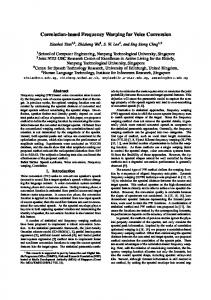
For high enough SNR the empirical mean-square-error (MSE) of MLE, WPA, and AMLE attains the CRB, whereas the MSE of (20) is approximately 0.5dB above the CRB. The performance curves of MLE and AMLE exhibit similar threshold values around 0dB, whereas the threshold for WPA is approximately 7dB higher. B. Performance versus M The performance versus M is studied in Figure 2 where the empirical MSE and the theoretical error variance for (18) and (20) are shown. As reference, the CRB and the empirical MSE for (17) are included in Figure 2. Here, the SNR is given by SNR= 20dB and the number of runs is 10000. An excellent agreement between the empirical results and the results predicted by theory may be noted. In general there are two minima of the variance curves, where the minimum corresponding to the lower M value results in slightly inferior performance. C. Performance versus N In Table I, the SNR threshold as function of N is shown for MLE, AMLE, and WPA. The same experiment conditions as above are considered. The threshold is measured as the location where the MSE starts to deviate from the CRB, based on performance curves similar to the ones in Figure 1 averaged out of 100 simulation runs. From the figures in Table I, one may note that the thresholds for MLE and AMLE are shifted to lower SNR as N increases. For the WPA, however, the threshold is shifted to higher SNR as N increases. See [5] for an explanation of this behavior.
VII. Conclusions A class of correlation based single tone frequency estimators has been derived utilizing an assumption on high SNR. The estimators are formulated in terms of differentiated autocovariances, and thus no additional unwrapping of the phase is required. A novel approximate maximum likelihood (AMLE) estimator has been derived, and alternative implementations of existing suboptimal estimators have been proposed. It has been shown that the performance of AMLE is nearly optimal, that is the error variance is close to the CRB for high and moderate SNR.
For high SNR, xk ≈ sk = Aeiωk , and thus xk ≃ |A|ei [xk ] . Inserting the latter expression for xk into (26) gives " N −1 ! N −1 !# X X i(ωk−6 [xk ]) i(6 [xk ]−ωk) Im |A|e |A|ke = 0 (27) k=0
k=1
Using the Taylor series expansion eix ≃ 1 + ix, a tedious but straightforward calculation solving for ω results in the estimator ! N −1 N −1 X X 6 6 [xk ] ω ˆ= 2 k 6 [xk ] − (N − 1) (28) N (N 2 − 1) k=1
k=0
The estimator in (28) is the estimator in [3]. In [3] it was observed that 6 [xk ] ≃ ωk + µ + vk where µ = arg[A] and vk is a real-valued white Gaussian noise. Thus the MLE of ω and µ is given by a least squares fit, that results in the estimator (28). References [1]
D.C. Rife and R.R. Boorstyn, “Single tone parameter estimation from discrete-time observations”, IEEE Transactions on Information Theory, Vol. IT-20, No. 5, pp. 591–598, 1974. [2] P. Stoica and R. Moses, Introduction to Spectral Analysis, Prentice-Hall, Englewood Cliffs, NJ, 1997. [3] S.A. Tretter, “Estimating the frequency of a noisy sinusoid by linear regression”, IEEE Transactions on Information Theory, Vol. IT-31, No. 6, pp. 832–835, 1985. [4] S. Kay, “Statistically/computationally efficient frequency estimation”, Proc. 1988 IEEE International Conference Acoustics, Speech, and Signal Processing, New York, NY, April 11-14, 1988, pp. 2292–2295. Extended version as “A fast and accurate single frequency estimator”, IEEE Transactions on Acoustics, Speech and Signal Processing, Vol. 37, No. 12, pp. 1987–1990, December 1989. [5] S.W. Lang and B.R. Musicus, “Frequency estimation from phase differences”, Proc. 1989 IEEE International Conference Acoustics, Speech, and Signal Processing, Glasgow, UK, May 23-26, 1989, pp. 2140–2143. [6] G.W. Lank, I.S. Reed and G.E. Pollon, “A semicoherent detection and Doppler estimation statistic”, IEEE Transactions on Aerospace and Electronic Systems, Vol. AES-9, pp. 151–165, 1973. [7] M.P. Fitz, “Further results in the fast estimation of a single frequency”, IEEE Transactions on Communications, Vol. 42, February/March/April No. 2/3/4, pp. 862–864, 1994. [8] L.B. Jackson, D.W. Tufts, F.K. Soong and R.M. Rao, “Frequency estimation by linear prediction”, Proc. 1978 IEEE International Conference on Acoustics, Speech, and Signal Processing, Tulsa, OK, April 10-12, 1978, pp. 352–356. [9] M. Luise and R. Reggiannini, “Carrier frequency recovery in alldigital modems for burst mode transmissions”, IEEE Transactions on Communications, Vol. 43, February/March/April No. 2/3/4, pp. 1169–1178, 1995. [10] P. H¨ andel, “Markov based single tone frequency estimation”, IEEE Transactions on Circuits and Systems – II Analog and Digital Signal Processing, to appear, 1997. [11] P. H¨ andel, A. Eriksson and T. Wigren, “Performance analysis of a correlation based single tone frequency estimator”, Signal Processing, Vol. 44, No. 2, pp. 223–231, June 1995.
36
MLE
WPA 80 −10LOG(MSE) (dB)
−10LOG(MSE) (dB)
80 60 40 20 0 −10
0
10 20 SNR (dB) AMLE
20
0
10 20 SNR (dB) Lank’s
30
0
10 20 SNR (dB)
30
80 −10LOG(MSE) (dB)
−10LOG(MSE) (dB)
40
0 −10
30
80 60 40 20 0 −10
60
0
10 20 SNR (dB)
60 40 20 0 −10
30
Fig. 1. The frequency error variance as a function of SNR for N = 24. The diagrams show empirical mean-square-error for the MLE, the weighted phase averager (WPA), the approximate MLE (17), and the estimator (20) with M = 16. In the lower diagrams the theoretical error variance is indicated by dashed lines.
−46
−47
10LOG(MSE) (dB)
−48
−49
−50
−51
−52
−53
−54 0
5
10
15
20
25
M Fig. 2. Error variance versus number of correlations used for (18) (dashed line) and (20) (dashed-dotted line). For (18) and (20) the empirical MSEs are depicted by “+” and “x”, respectively. As reference, the CRB (solid line), the lower bound (22)-(25) (solid line), and empirical MSE of AMLE (“o”) are shown.