B B330 (1990), 465; P. Christe and G. Mussardo Int. J. Mod. Phys. A5 (1990), 1025; H. W. Braden, E. Corrigan, P. E. Dorey, R. Sasaki, Nucl. Phys. B338 (1990) ...
ISAS/EP/92/236
Correlation Functions in 2-Dimensional Integrable
arXiv:hep-th/9212119v1 19 Dec 1992
Quantum Field Theories
G. Mussardo International School for Advanced Studies, and Istituto Nazionale di Fisica Nucleare 34014 Trieste, Italy
Abstract In this talk I discuss the form factor approach used to compute correlation functions of integrable models in two dimensions. The Sinh-Gordon model is our basic example. Using Watson’s and the recursive equations satisfied by matrix elements of local operators, I present the computation of the form factors of the elementary field φ(x) and the stress-energy tensor Tµν (x) of the theory.
1
Introduction
Important progress in Quantum Field Theories has been made in recent years by studying two dimensional relativistic models. The reason essentially lays in the successful application of several non-perturbative approaches which lead to exact solutions of the quantum field dynamics. In this talk I am concerned with the determination of multi-point correlation functions of local operators for a massive field theory Gn (r1 , r2 , . . . , rn ) = < Oi1 (r1 ) Oi2 (r2 ) . . . Oin (rn ) > .
(1.1)
My basic example will the the Sinh-Gordon model which is discussed in a work made in collaboration with A. Fring and P. Simonetti [1]. For two-dimensional systems, there is usually a special limit where the computation of the Gn ’s is greatly simplified. This is the ultraviolet asymptotic regime of the correlation functions, defined by |ri − rj | ≪ ξ . where the correlation length is given by ξ = m−1 . This regime can be equivalently reached by keeping finite values of the distances but taking the limit ξ → ∞. Either ways, a scale invariant behaviour occurs in the model and the resulting 2-D infinitedimensional conformal symmetry induces a system of linear differential equations satisfied by the correlators Gn [2]. Their solution provides an explicit expression for the correlation functions of the theory in the ultraviolet regime [2, 3, 4]. However, the behaviour of correlation functions in the cross-over region |ri − rj | ≃ ξ , and in the infrared limit |ri − rj | ≫ ξ , 1
is more complicated. Consider, for instance, the case of two-point correlation functions < Oi (r) Oi (0) > =
1 Φi (mr) . r ηi
(1.2)
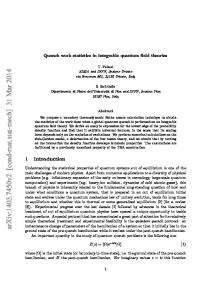
With this parametrization, the exponent ηi is usually identified with twice the anomalous dimension of the field Oi whereas Φi (x) is a scaling function∗ of the variable x = mr. Although conformal invariance severely restricts the possible values of ηi and gives quite powerful classification of the ultraviolet behaviours of two-dimensional models, the computation of the scaling functions Φi (r) is, on the contrary, quite difficult. There exists, however, a large class of relativistic models where the determination of the scaling functions can be explicitly worked out. This is the case of the massive integrable systems whose dynamics is strongly constrained by an infinite number of integrals of motion. In particular, the S-matrix of these models presents factorization and elasticity properties and can be explicitly constructed [5-11]. In order to compute multi-point correlators for massive integrable models, we may exploit their spectral representation, i.e. their decomposition into an infinite sum over intermediate multi-particle contributions (fig. 1). For instance, the two-point function of a hermitian scalar operator Oi (x) in real Euclidean space can be written as† hOi (x) Oi (0)i = =
∞ Z X
n=0 ∗
∞ Z X
n=0
dβ1 . . . dβn < 0|Oi (x)|β1 , . . . , βn >in n!(2π)n
in
< β1 , . . . , βn |Oi (0)|0 >
n X dβ1 . . . dβn Oi 2 | F (β . . . β ) | exp −mr cosh βi 1 n n n!(2π)n i=1
!
,
(1.4)
Scaling functions can be introduced as well for the n-point correlators. We concentrate our
discussion on the two-point functions for clarity and simplicity. † β is the rapidity variable, related to the two-dimensional momentum by p0 = m cosh β , p1 = m sinh β .
2
(1.3)
where r denotes the radial distance r =
q
x20 + x21 .
'$
.. ..
Oi (x)
&%
'$
Oi (0)
&%
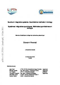
Figure 1 The functions FnOi (β1 , β2 , . . . , βn ) = < 0|Oi (0)|β1 , β2 , . . . , βn >in
(1.5)
are the form factors of the operator Oi (fig. 2).
@
βn
β1
'$ @
@ βn−1
ϕi (0)
β2 .. &% . β 3 @ @ @
Figure 2
Analytic properties of the form factors have been investigated by several authors and particularly important contributions can be found in [13-19]. As I will show in 3
the following, the form factor approach is a successful method in order to compute correlation functions. The expansion of the correlators in terms of the number of intermediate particles rather than in a perturbative series of the coupling constant presents, in fact, several advantages. First of all, the form factors take into account coupling constant dependence of correlation functions to all order in perturbation theory. Secondly, expressions like that one in eq. (1.4) are fast convergent series in the number N of intermediate particles even for moderate value of the distance and therefore, for practical applications, it is often sufficient to compute the form factors of the operator Oi with few external particles. Moreover, this spectral representation of two-point functions formally coincides with the grand partition function of a one-dimensional gas system, as noticed in [17, 19]. Hence, one can borrow successful techniques developped for one-dimensional system in order to extract non-perturbative parameters of the theory. For instance, as shown in [17, 19], the anomalous dimension of the operator O in the ultraviolet limit is equal to the pressure of the corresponding one-dimensional gas at one specific value of the fugacity. I will focalize on the form factor approach for the Sinh-Gordon model, described by the Lagrangian L =
1 m2 (∂µ φ)2 − 20 cosh g φ(x) . 2 g
(1.6)
The SG model belongs to the class of Toda Field Theory constructed on the simplylaced root systems, in this case A1 . The reason why I will consider this model is its simplicity which allows us to understand the basic principles of the computation without being masked by algebraic complicancies. Let us discuss initially the basic features of this theory.
4
2
The Sinh-Gordon Theory
The SG model is the simplest example of an affine Toda Field Theories [20], possessing a Z2 symmetry φ → −φ. By an analytic continuation in g, i.e g → ig, it can formally be mapped to the Sine-Gordon model. There are numerous alternative viewpoints for the Sinh-Gordon model. First, it can be regarded either as a perturbation of the free massless conformal action by means of the relevant operator‡ cosh gφ(x). Alternatively, it can be considered as a perturbation of the conformal Liouville action S =
Z
d2 x
�
1 (∂µ φ)2 − λegφ 2
�
(2.1)
by means of the relevant operator e−gφ or as a conformal affine A1 -Toda Theory [21] in which the conformal symmetry is broken by setting the free field to zero. In a perturbative approach to the quantum field theory defined by the Lagrangian (1.6), the only ultraviolet divergences which occur in any order in g come from tadpole graphs and can be removed by a normal ordering prescription with respect to an arbitrary mass scale M. All other Feynman graphs are convergent and give rise to finite wave function and mass renormalisation. The coupling constant g does not renormalise. An essential feature of the Sinh-Gordon theory is its integrability, which in the classical case can be established by means of the inverse scattering method [24]. In order to obtain the expressions of the (classical) conserved currents one can use B¨acklund transformation, as shown in [1], and obtains an infinite set of conservation laws ∂z Ts+1 = ∂z Θs−1 . ‡
(2.2)
Although the anomalous dimension of this operator (computed with respect to the free confor-
mal point), is negative, ∆ = −g 2 /8π, the resulting theory is unitary. This is due to the existence of non a nonzero vacuum expectation values of some of the fields Oi in the theory. A detailed discussion of this point can be found in [18].
5
The corresponding charges Qs are given by Qs =
I
[Ts+1 dz + Θs−1 dz] .
(2.3)
The integer-valued index s which labels the integrals of motion is the spin of the operators. Non-trivial conservation laws are obtained for odd values of s s = 1, 3, 5, 7, . . .
(2.4)
In analogy to the Sine-Gordon theory [23], an infinite set of conserved charges Qs with spin s given in (2.4) also exists for the quantized version of the Sinh-Gordon theory. They are diagonalised by the asymptotic states with eigenvalues given by Qs |β1 , . . . , βn > = χs
n X i=1
esβi |β1 , . . . , βn > ,
(2.5)
where χs is the normalization constant of the charge Qs . The existence of these higher integrals of motion precludes the possibility of production processes and hence guarantees that the n-particle scattering amplitudes are purely elastic and factorized into n(n − 1)/2 two-particle S-matrices. The exact expression for the Sinh-Gordon theory is given by [10] S(β, B) =
tanh 12 (β − i πB ) 2 πB , 1 tanh 2 (β + i 2 )
(2.6)
where B is the following function of the coupling constant g B(g) =
2g 2 . 8π + g 2
(2.7)
This formula has been checked against perturbation theory in ref. [10] and can also be obtained by analytic continuation of the S-matrix of the first breather of the Sine-Gordon theory [5]. For real values of g the S-matrix has no poles in the physical sheet and hence there are no bound states, whereas two zeros are present at the crossing symmetric positions β =
i πB 2 i π(2−B) 2 6
(2.8)
An interesting feature of the S-matrix is its invariance under the map [11] B →2−B
(2.9)
i.e. under the strong-weak coupling constant duality g→
8π . g
(2.10)
This duality is a property shared by the unperturbed conformal Liouville theory (2.1) [22] and it is quite remarkable that it survives even when the conformal symmetry is broken.
3
Form Factors
The form factors (FF) are matrix elements of local operators between the vacuum and n-particle in-state FnO (β1 , β2 , . . . , βn ) = < 0|O(0)|β1 , β2 , . . . , βn >in .
(3.1)
For local scalar operators O(x), relativistic invariance implies that Fn are functions of the difference of the rapidities. Except for the poles corresponding to the oneparticle bound states in all sub-channels, we expect the form factors Fn to be analytic inside the strip 0 < Imβij < 2π. The form factors of a hermitian local scalar operator O(x) satisfy a set of functional equations, known as Watson’s equations [12], which for integrable systems assume a particularly simple form Fn (β1 , . . . , βi , βi+1 , . . . , βn ) = Fn (β1 , . . . , βi+1 , βi , . . . , βn )S(βi − βi+1 ) , Fn (β1 + 2πi, . . . , βn−1 , βn ) = Fn (β2 , . . . , βn , β1 ) =
n Y
i=2
(3.2)
S(βi − β1 )Fn (β1 , . . . , βn ) .
The first equation states that as a result of the commutation of two particles in the asymptotic state we get a scattering process whereas the second equation fixes the 7
discontinuity of the functions Fn on the cuts β1i = 2πi. In the case n = 2, eqs. (3.2) reduce to F2 (β)
= F2 (−β)S2 (β) ,
(3.3)
F2 (iπ − β) = F2 (iπ + β) .
The general solution of Watson’s equations for diagonal S-matrix systems can always be brought into the form [13] Fn (β1 , . . . , βn ) = Kn (β1 , . . . , βn )
Y
Fmin (βij ) ,
(3.4)
iin = √ . 2
(4.1)
For the even sector, an important operator is given by the energy-momentum tensor Tµν (x) = 2π (: ∂µ φ∂ν φ − gµν L(x) :)
(4.2)
where : : denotes the usual normal ordering prescription with respect an arbitrary mass scale M. Its trace Tµµ (x) = Θ(x) is a spinless operator whose normalization is fixed in terms of its two-particle form factor F2Θ (β12 = iπ) =
out
< β1 | Θ(0) | β2 >in = 2πm2 ,
(4.3)
where m is the physical mass. In the following we shall compute the form factors of the operators φ(x) and Θ(x). Employing the parameterization (3.11), the recursive equations (3.14) take on the form (−)n Qn+2 (−x, x, x1 , . . . , xn ) = xDn (x, x1 , x2 , . . . , xn ) Qn (x1 , x2 , . . . , xn ) 11
(4.4)
where we have introduced the function n h n h i i Y Y −i (x − ωxi )(x + ω −1 xi ) (x + ωxi )(x − ω −1xi ) − Dn = 4 sin(πB/2) i=1 i=1 (4.5)
!
with ω = exp(iπB/2). The normalization constants for the form factors of odd and even operators are conveniently chosen to be H2n+1 = H1
4 sin(πB/2) Fmin (iπ, B)
!n
H2n = H2
4 sin(πB/2) Fmin (iπ, B)
!n−1
(4.6)
where H1 and H2 are the initial conditions, fixed by the nature of the operator. Using the generating function (3.13) of the symmetric polynomials, the function Dn can be expressed as n X πB 2n−l−k (n) (n) 1 x σl σk . (−1)l sin (k − l) Dn = 2 sin(πB/2) l,k=0 2
�
�
(4.7)
As function of B, Dn is invariant under B → −B. As shown in [1], the symmetric polynomials Q2n+1 entering the form factors of the elementary field φ(x) can be factorized as (2n+1)
Q2n+1 (x1 , . . . , x2n+1 ) = σ2n+1 P2n+1 (x1 , . . . , x2n+1 )
n>0 ,
(4.8)
whereas the analogous polynomials entering the form factors of the trace of the stress-energy tensor can be written as (2n) (2n) σ2n−1
Q2n (x1 , . . . , x2n ) = σ1
P2n (x1 , . . . , x2n )
n>1 .
(4.9)
Pn (x1 , . . . , xn ) is a symmetric polynomial of total degree n(n − 3)/2 and of degree n − 3 in each variable xi . Using the following property of the elementary symmetric polynomials (n+2)
σk
(n)
(n)
(−x, x, x1 , . . . , xn ) = σk (x1 , x2 , . . . , xn ) − x2 σk−2 (x1 , x2 , . . . , xn ) , 12
(4.10)
the recursive equations (4.4) can then be written in terms of the Pn as (−)n+1 Pn+2 (−x, x, x1 , . . . , xn ) =
1 Dn (x, x1 , x2 , . . . , xn ) Pn (x1 , x2 , . . . , xn ) . x (4.11)
Using the recursive equations (4.11) and the transformation property of the elementary symmetric polynomials (4.10), the explicit expressions of the first polynomials Pn (x1 , . . . , xn ) are given by¶ P3 (x1 , . . . , x3 ) = 1 P4 (x1 , . . . , x4 ) = σ2 P5 (x1 , . . . , x5 ) = σ2 σ3 − c21 σ5
(4.12)
P6 (x1 , . . . , x6 ) = σ3 (σ2 σ4 − σ6 ) − c21 (σ4 σ5 + σ1 σ2 σ6 − σ3 σ6 ) P7 (x1 , . . . , x7 ) = σ2 σ3 σ4 σ5 − c21 (σ4 σ52 + σ1 σ2 σ5 σ6 + σ22 σ3 σ7 − c21 σ2 σ5 σ7 ) + −c2 (σ1 σ2 σ4 σ7 + σ3 σ5 σ6 − c2 σ1 σ6 σ7 ) + c21 c22 σ72 where c1 = 2 cos(πB/2) and c2 = 1 − c21 . Expression of the higher Pn are easily computed by an iterative use of eqs. (4.4). For practical application the first representatives of Pn are sufficient to compute with a high degree of accuracy the correlation functions of the fields. In fact, the n-particle term appearing in the correlation function of the fields (1.4) behaves as e−n(mr) and for quite large values of mr the correlator is dominated by the lowest number of particle terms. This conclusion is also confirmed by an application of the c-theorem which I discuss at the end of the talk. It is interesting to notice that closed expressions for Pn can be found for particular values of the coupling constant. 4.0.1 ¶
The Self-Dual Point
The upper index of the elementary symmetric polynomials entering Pn is equal to n and we
suppress it, in order to simplify the notation.
13
The self-dual point in the coupling constant manifold has the special value B
�√
�
8π = 1 .
(4.13)
The two zeros of the S-matrix merge together and the function Dn (x, x1 , x2 , . . . , xn ) acquires the particularly simple form Dn (x|x1 , x2 . . . , xn ) =
n X
k+1
(−1)
k=0
kπ n−k (n) x σk sin 2
!
n X
!
lπ (n) . (−1) cos xn−l σl 2 l=0 (4.14) l
In this case the general solution of the recursive equations (4.11) is given by [1] Pn (x1 , x2 , . . . , xn ) = det A(x1 , x2 , . . . , xn )
(4.15)
where A is an (n − 3) × (n − 3) matrix whose entries are Aij (x1 , x2 , . . . , xn ) = i.e.
A=
(n) σ2j−i+1
σ2 0
σ6 0
0
σ3 0
1
0
0 .. .
π cos (i − j) 2
0 .. .
�
�
,
(4.16)
···
σ7 · · ·
σ4 0
σ1 .. .
2
···
σ5 · · · .. .. . .
(4.17)
This can be proved by exploiting the properties of determinants. 4.0.2
The “Inverse Yang-Lee” Point
A closed solution of the recursive equations (4.11) is also obtained for � √ � 2 B 2 π = . 3
(4.18)
The reason is that, for this particular value of the coupling constant the S-matrix of the Sinh-Gordon theory coincides with the inverse of the S-matrix SYL (β) of the Yang-Lee model [8] or, equivalently 2 S(β, − ) = SYL (β) . 3 14
(4.19)
Since the recursive equations (4.11) are invariant under B → −B (see sect. 4.2), a solution is provided by the same combination of symmetric polynomials found for the Yang-Lee model [16, 18], i.e. Pn (x1 , x2 , . . . , xn ) = det B(x1 , x2 , . . . , xn )
(4.20)
with the following entries of the (n − 3) × (n − 3)-matrix B Bij = σ3j−2i+1 .
5
(4.21)
Form factors and c-theorem
The Sinh-Gordon model can be regarded as deformation of the free massless theory with central charge c = 1. This fixed point governs the ultraviolet behaviour of the model whereas the infrared behaviour corresponds to a massive field theory with central charge c = 0. Going from the short- to large-distances, the variation of the central charge is dictated by the c-theorem of Zamolodchikov [26]. An integral version of this theorem has been derived by Cardy [27] and related to the spectral representation of the two-point function of the trace of the stress-energy tensor in [28, 29], i.e. ∆c =
Z
0
∞
dµ c1 (µ) ,
(5.1)
where c1 (µ) is given by c1 (µ) =
6 1 Im G(p2 = −µ2 ) , π 2 µ3
G(p2 ) =
Z
(5.2)
d2 x e−ipx˙ < 0|Θ(x)Θ(0)|0 >conn .
Inserting a complete set of in-state into (5.2), we can express the function c1 (µ) in Θ terms of the form factors F2n
c1 (µ) =
∞ 1 12 X µ3 n=1 (2n)!
× δ(
X
Z
dβ1 . . . dβ2n Θ | F2n (β1 , . . . , β2n ) |2 (2π)2n
m sinh βi ) δ(
X i
i
15
m cosh βi − µ) .
(5.3)
B
g2 4π
∆ c(2)
1 500
2 999
0.9999995
1 100
2 199
0.9999878
1 10
2 19
0.9989538
3 10
6 17
0.9931954
2 5
1 2
0.9897087
1 2
2 3
0.9863354
2 3
1
0.9815944
7 10
14 13
0.9808312
4 5
4 3
0.9789824
1
2
0.9774634
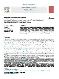
For the Sinh-Gordon theory ∆c = 1 and it is interesting to study the convergence of this series increasing the number of intermediate particles. For the two-particle contribution, we have the following expression ∆c
(2)
=
3 2 2Fmin (iπ)
Z
∞
0
dβ |Fmin (2β)|2 . 4 cosh β
(5.4)
The numerical results for different values of the coupling constant g 2 /4π are listed in the table below It is evident that the sum rule is saturated by the two-particle form factor also for large values of the coupling constant. Hence, the expansion in the number of intermediate particles results in a fast convergent series, as it is confirmed by the computation of the next terms involving the form factor with four and six particles.
16
6
Conclusions
The computation of the Green functions is a central problem in a Quantum Field Theory. For integrable models, a promising approach to this question is given by the bootstrap principle applied to the computation of the matrix elements of local operators. It would be interesting to use this approach in order to derive differential equations satisfied by the quantum correlators and also to classify the operator content of a quantum integrable field theory.
Acknowledgments I would like to thank A. Fring and P. Simonetti for our collaboration on this project and S. Elitzur and A. Schwimmer for useful discussions.
References [1] A. Fring,
G. Mussardo and P. Simonetti,
Form Factors for Inte-
grable Lagrangian Field Theories, the Sinh-Gordon Model, ISAS/EP/92-146, Imperial/TP/91-92/31, to appear on Nucl. Phys. B. [2] A.A. Belavin, A.M. Polyakov and A.B. Zamolodchikov, Nucl. Phys. B241 (1984), 333. [3] Vl.S. Dotsenko and V.A. Fateev, Nucl. Phys. B240 [FS 12] (1984), 312; Nucl. Phys. B251 [FS 13] (1985), 691; Phys. Lett. B 154 (1985), 291. [4] C. Itzykson, H. Saleur and J.B. Zuber, Conformal Invariance and Applications to Statistical Mechanics, (World Scientific, Singapore 1988). [5] A.B. Zamolodchikov, Al.B. Zamolodchikov, Ann.Phys. 120 (1979), 253. 17
[6] A.B. Zamolodchikov, in Advanced Studies in Pure Mathematics 19 (1989), 641; Int. J. Mod. Phys.A3 (1988), 743. [7] R. K¨oberle and J.A. Swieca, Phys. Lett. 86B (1979), 209; A.B. Zamolodchikov, Int. J. Mod. Phys. A3 (1988), 743; V. A. Fateev and A.B. Zamolodchikov, Int. J. Mod. Phys. A5 (1990), 1025. [8] J.L. Cardy, G. Mussardo, Phys. Lett. B225 (1989) , 275. [9] G. Mussardo, Phys. Rep. 218 (1992), 215. [10] A.E. Arinshtein, V.A. Fateev and A.B. Zamolodchikov, Phys. Lett. 87B (1979), 389. [11] P. Christe and G. Mussardo, Nucl.Phys. B B330 (1990), 465; P. Christe and G. Mussardo Int. J. Mod. Phys. A5 (1990), 1025; H. W. Braden, E. Corrigan, P. E. Dorey, R. Sasaki, Nucl. Phys. B338 (1990), 689; H. W. Braden, E. Corrigan, P. E. Dorey, R. Sasaki, Nucl. Phys. B356 (1991), 469. [12] K.M. Watson, Phys. Rev. 95 (1954), 228. [13] B. Berg, M. Karowski, P. Weisz, Phys. Rev. D19 (1979), 2477; M. Karowski, P. Weisz, Nucl. Phys. B139 (1978), 445; M. Karowski, Phys. Rep. 49 (1979), 229; [14] F. A. Smirnov, in Introduction to Quantum Group and Integrable Massive Models of Quantum Field Theory, Nankai Lectures on Mathematical Physics, World Scientific 1990. [15] F.A. Smirnov, J. Phys. A17 (1984), L873; F.A. Smirnov, J. Phys. A19 (1984), L575; A.N. Kirillov and F.A. Smirnov, Phys. Lett. B198 (1987), 506; A.N. Kirillov and F.A. Smirnov, Int. J. Mod. Phys. A3 (1988), 731.
18
[16] F.A. Smirnov, Nucl. Phys. B337 (1989), 156; Int. J. Mod. Phys. A4 (1989), 4213. [17] V.P. Yurov and Al. B. Zamolodchikov, Int. J. Mod. Phys. A6 (1991), 3419. [18] Al.B. Zamolodchikov, Nucl. Phys. B348 (1991), 619. [19] J.L. Cardy and G. Mussardo, Nucl. Phys. B340 (1990), 387. [20] A.V. Mikhailov, M.A. Olshanetsky and A.M. Perelomov, Comm. Math. Phys. 79 (1981), 473. [21] O. Babelon and L. Bonora, Phys. Lett. B244 (1990), 220. [22] P. Mansfield, Nucl. Phys. B222 (1983), 419. [23] R. Sasaki and I. Yamanaka, in Advanced Studies in Pure Mathematics 16 (1988), 271. [24] L.D. Faddev and L.A. Takhtajan, Hamiltonian Method in the Theory of Solitons, (Springer, N.Y., 1987). [25] I.G. MacDonald, Symmetric Functions and Hall Polynomials (Clarendon Press, Oxford, 1979). [26] A.B. Zamolodchikov, JEPT Lett. 43 (1986), 730. [27] J.L. Cardy, Phys. Rev. Lett. 60 (1988), 2709. [28] A. Cappelli, D. Friedan and J.L. Latorre, Nucl. Phys. B352 (1991), 616. [29] D.Z. Freedman, J.I. Latorre and X. Vilasis, Mod. Phys. Lett. A6 (1991), 531.
19