Mar 31, 2014 - We propose a boundary thermodynamic Bethe ansatz calculation technique ... thermodynamic limit a concentration of zeroes around particular ...
arXiv:1403.7450v2 [cond-mat.stat-mech] 31 Mar 2014
Quench work statistics in integrable quantum field theories T. Palmai SISSA and INFN, Sezione Trieste via Bonomea 265, 34136 Trieste, Italy S. Sotiriadis Dipartimento di Fisica dell’Universit` a di Pisa and INFN, Sezione Pisa 56127 Pisa, Italy
Abstract We propose a boundary thermodynamic Bethe ansatz calculation technique to obtain the statistics of the work done when a global quantum quench is performed on an integrable quantum field theory. We derive an analytic expression for the lowest edge of the probability density function and find that it exhibits universal features, in the sense that its scaling form depends only on the statistics of excitations. We perform numerical calculations on the sinh-Gordon model, a deformation of the free boson theory, and we obtain that by turning on the interaction the density function develops fermionic properties. The calculations are facilitated by a previously unnoticed property of the TBA construction.
1
Introduction
Understanding the statistical properties of quantum systems out of equilibrium is one of the main challenges of modern physics. Apart from numerous applications to a diversity of physical problems (e.g. inflationary expansion of the early universe in cosmology, large-scale quantum computation) and experiments (e.g. heavy-ion collision, dynamics of cold atomic gases), this branch of physics is inherently related to the fundamental long-standing question of how and under what conditions a quantum system, that is prepared in an out of equilibrium initial state and evolves under the quantum mechanical law of unitary evolution, tends for long times to equilibrium and whether this is thermal or some generalised equilibrium [2] (for a review [3]). Experimental progress over the last decade [1] followed by advances in the theoretical treatment of out of equilibrium quantum physics have opened a unique opportunity to tackle such questions. A special protocol that has concentrated a great part of attention for its relatively simple theoretical treatment and experimental feasibility is the quantum quench protocol: an instantaneous change of parameters of the hamiltonian of a system so that it initially lies in the ground state of the pre-quench hamiltonian while it evolves under the post-quench hamiltonian. An important quantity in the study of quantum quench problems is the following one Z(z) = hΩ|e−Hz |Ωi
(1)
where |Ωi is the initial state (or boundary-in-time state), i.e. the ground state of the pre-quench hamiltonian, and H the post-quench hamiltonian. For imaginary values z = it this function 1
gives the overlap between the initial and the evolved state after time t, the Loschmidt amplitude, whose norm square is the Loschmidt echo [4, 5]. This overlap is essentially the characteristic function of the probability density function P (W ) of the statistics of the work done [7, 8, 13, 15] (differing in a constant factor and shift). Knowledge of this distribution amounts to knowledge of all probabilities to excite each post-quench energy level, which is all that is needed in order to calculate the long time averages of observables [22] or their asymptotic values provided they become stationary [26]. On the other hand, for positive real values of z = R the above quantity is the partition function of a system defined in a 2d strip of width R with boundary conditions |Ωi on both edges. Z(z) in the complex plane is also an interesting subject of study. In lattice models in particular, since Z(z) is an entire function [6], its zeroes in the complex z-plane determine completely the non-analytic part of the associated free energy. It has been shown that, in the thermodynamic limit a concentration of zeroes around particular points of the imaginary axis (real t-axis) leads to non-analytic behaviour in the free energy [21]. This has been demonstrated for a quench across the critical point of the Ising model, exploiting its mapping to free fermions (where however the continuum limit tames the singularities of the free energy corresponding to zeroes of Z(z) into square root branch points). It was proposed that such zeroes (or branch points) of Z(z) play a role analogous to that of Fisher zeroes in ordinary phase transitions [21]. This non-analytic behaviour was later shown to be robust under the inclusion of nonintegrable interactions, irrelevant or relevant in the RG sense, using the tDMRG numerical method [39]. More recently it was also shown that such non-analyticities are caused more generally by a crossing of eigenvalues in the spectrum of the transfer matrix [42]. Further progress in the analytical calculation of the above quantity for integrable spin chains was made using Algebraic Bethe-Ansatz techniques [22, 41]. If the analytical continuation of the complex variable z = R + it from real to imaginary values is not prevented by the presence of zeroes (that correspond to logarithmic singularities of the associated free energy), it is possible to calculate the work probability distribution P (W ) from the boundary partition function Z(R). In this way universal behaviour associated with the critical Casimir effect in the boundary formulation of the problem can be connected to universal properties of P (W ) in the limit of massless postquench hamiltonian, in particular properties of its lowest excitation threshold [13, 17, 15]. The Loschmidt echo has been calculated in the context of quantum quench and related problems in several other studies relative to spin chains, conformal field theories and other models that are essentially equivalent to non-interacting ones [29, 30, 31, 32, 33, 34, 35, 36, 37, 38]. It is clear that for a general relativistic Integrable Quantum Field Theory (IQFT) and special initial states, the function (1), viewed as the partition function of the strip boundary problem for real values of z, can be calculated using the so-called boundary Thermodynamic Bethe Ansatz (BTBA) [43, 44]. In the BTBA the boundaries are represented by states that preserve the integrability of the bulk of the system (boundary integrable states) and were shown to be of the following form [23] � �Z ∞ dθ † † K(θ)Z (−θ)Z (θ) |0i (2) exp 2π 0 The operators Z(θ), Z † (θ) are the Zamolodchikov-Faddeev operators [45, 46], strings of which acting on the vacuum create asymptotic scattering states, that constitute an eigenstate basis of the IQFT. K(θ) in the boundary integrable problem satisfies the so-called boundary crossunitarity condition and is related to the reflection matrix (θ is the rapidity variable, a convenient 2
reparametrisation of the momentum of single particle excitations, i.e. its energy’s and momentum’s being E = m cosh θ and p = m sinh θ, respectively). For simplicity, in the above equation and in all that follows we restrict ourselves to an IQFT with a single particle species, as is the sinh-Gordon (shG) model. The Dirichlet state, a typical example of a boundary integrable state, defined as the state annihilated by the physical field φ and thus having vanishing field fluctuations, is of the above form with K(θ) = KD (θ) known exactly [24, 25]. The initial state of a global quantum quench in IQFTs is given, in certain important special cases, by this same boundary integrable form (2). Such cases are those of free theories and when the pre-quench mass tends to infinity. In the latter case the field fluctuations vanish and therefore the initial state is exactly the Dirichlet state. This state requires careful ultraviolet regularization, since otherwise it leads to divergent physical observables. It has been recently argued [28] that for a quantum quench in the shG model from a large but finite pre-quench mass m0 and zero interaction to an arbitrary post-quench mass m and arbitrary interaction, one obtains as initial state a modified Dirichlet state that is approximately given by the same form (2) with amplitude K(θ) = KD (θ)KF B (θ) where KF B (θ) is the amplitude that corresponds to a free bosonic quantum quench of the mass from m0 to m. This state is free from ultraviolet divergences and consistent with the requirements of a quantum quench. In complete generality, the situation seems to be more complicated [27]: the extensivity of the conserved charges in the initial state introduces certain constraints for the amplitudes of excitations contained in it, at least in the limit of large number of particles [22], but those constraints are more general than the precise special form (2). Considering all the above, in this work we propose a derivation of the Loschmidt amplitude and thus the work statistics relative to a global quench in IQFTs by means of the boundary TBA solved on the imaginary axis. Since the TBA is an integral equation representation, we a priori expect that the analytical continuation would give the correct Loschmidt echo. Indeed, a similar approach has been successfully used before for the calculation of excitation energies in IQFT [9, 10, 11, 12]. We perform this calculation in the sinh-Gordon model, arguably the simplest relativistic IQFT with non-trivial S-matrix. While this serves as a demonstration of the approach, it also allows us to see the effects of turning on the interaction on the thermodynamics of a quench in a quantum field theory. On the other hand, it can be considered as the first step for the application to a quench in the sine-Gordon model, which can be obtained by analytical continuation of the interaction coupling parameter of the shG model from real to imaginary values. A quantum quench in the sine-Gordon model can actually be experimentally implemented, for example in systems of split 1d Bose-Einstein quasi-condensates that interact through a longitudinal potential barrier that behaves like a Josephson junction [47, 48]. In what follows we expose general properties about the statistics of the work done when performing a quantum quench, then we introduce the thermodynamic Bethe ansatz, followed by a discussion of its continuation to imaginary temperatures, both from a theoretical and a numerical point of view. Then we discuss results for the work statistics of integrable field theories, in particular the sinh-Gordon model. We find that the first peak in the probability density function is not affected by the interaction and we give it in an analytic form. Then we discuss global mass quenches from large but finite initial masses in the free bosonic, free fermionic and the sinh-Gordon models. We determine that while the moments of the distribution, in particular the mean, are only changed slightly by turning on the interaction, the details are modified. This can be seen on the first edge, which develops a fermionic, positive edge singularity exponent 3
opposed to the bosonic negative one. The last section is reserved for conclusions.
2 2.1
Formulation Work statistics of a quantum quench
Consider a closed quantum system in a d-dimensional box of edge length L (d is the number of spatial dimensions) with periodic boundary conditions, undergoing a quench from the Hamiltonian H0 to H. Before the quench the system lies in the ground state |Ωi of the Hamiltonian H0 . One can treat the quench as a thermodynamic transformation and ask how much work is done on the system. Since the system is closed the change in energy equals to the work W . The quench is a non-equilibrium protocol and the work is stochastic. The probability distribution of it is defined as X P (W ) = δ(W − EΨ + Egs,0 ) |hΨ|Ωi|2 (3) all eigenstates |Ψi
where |Ψi is any eigenstate of the post-quench Hamiltonian, EΨ the corresponding energy eigenvalue and Egs,0 the energy of the pre-quench ground state |Ωi. The characteristic function G(t) of this probability distribution is the inverse Fourier transform Z ∞ dW e−iW t P (W ) (4) G(t) = −∞
which, using the previous definition, can be readily shown to be equal to X G(t) = ei(Egs,0 −EΨ )t |hΨ|Ωi|2 |Ψi
= eiEgs,0 t hΩ| e−iHt |Ωi
(5)
The last expression is the Loschmidt amplitude: the overlap between the state e−iHt |Ωi, which is the evolution of the initial state under the post-quench Hamiltonian H for time t, and the state e−iH0 t |Ωi, which is its evolution under the pre-quench Hamiltonian H for the same time t. On the other hand, performing the Wick rotation t → −iR, the resulting quantity is the moment generating function of the distribution and can be identified with the partition function of the system confined in a slab of width R with both boundary states equal to |Ωi. The latter has been extensively studied in the context of the Casimir effect. The corresponding free energy per volume f (R) ≡ − limL→∞ L−d log G(R) can be split into the following three parts according to their behaviour for large R f (R) = fb R + 2fs + fC (R) In the above fb and fs are the bulk and surface contributions, while the remaining part fC (R) decays for large R. In the original quantum quench problem, fb corresponds to the difference in the ground state energies of the post- and pre-quench Hamiltonians per volume, fb = (Egs − Egs,0 )L−d , while fs is related to the squared norm of the so-called fidelity |h0|Ωi| between these states, fs = −L−d log |h0|Ωi| where |0i is the post-quench ground state.
4
The cumulants (equivalent to the moments) of the probability distribution P (W ) are given by the logarithmic derivatives of its characteristic function at t = 0 � �n d n log G(t) κn = i dt t=0
Note that since log G(t) is extensive, all cumulants κn are extensive too, which means in particular that, increasing the system size L, the relative variance of P (W ) tends to zero and in the thermodynamic limit becomes a narrow bell-shaped distribution characterised by its mean value and variance. Note however, that in finite volume a more careful analysis predicts exponential corrections to the cumulants. The qualitative behaviour of P (W ) can be easily inferred by considering the energy absorption that corresponds to any of the possible transitions from the initial state to eigenstates of the post-quench Hamiltonian. The lowest energy absorption corresponds to the transition from the initial state to the post-quench ground state |0i, which therefore appears in P (W ) as a Dirac δ-function peak at the value W = Egs − Egs,0 with amplitude given by the squared norm of the so-called fidelity |h0|Ωi| between these states. From now on we will measure the work from the position of this lowest Dirac δ-function peak, i.e. we will subtract the ground state energy difference from the work W . The next lowest energy absorption corresponds to the transition to the lowest post-quench excitation that is allowed. For a massive post-quench Hamiltonian, like the sinh-Gordon Hamiltonian, the lowest excitations are separated from the ground state by the energy gap m i.e. the mass of the lightest quasi-particle excitations. However since the initial state is translationally invariant and due to the conservation of the momentum, only transitions to excitations with zero total momentum are allowed. Therefore, unless the post-quench Hamiltonian contains bound-state excitations which have zero momentum, the lowest allowed transition corresponds to the creation of two quasi-particles with opposite momenta ±k, k ≥ 0. This means that P (W ) exhibits a lowest threshold at 2m above which there is a continuous absorption spectrum corresponding to the continuous variable k. The shape of the absorption spectrum above this lowest threshold depends on the excitation amplitudes, the dimensionality d and the nature of the excitations (i.e. the statistics, bosonic or fermionic, and the parameters of their dispersion relation). At the vicinity of the threshold P (W ) exhibits an edge-singularity, typically appearing as a sharp peak. Provided that the analytic continuation R → it of the results for the Casimir free energy is valid, it can be shown that the edge-singularity exhibits universal behaviour controlled by the large R behaviour of fC (R). In more detail, just above the threshold the distribution exhibits a power-law form with an exponent that depends only on the dimensionality and the particle statistics. In 1d the edge exponent is −1/2 for bosons and +1/2 for fermions (for details, see below). If the excitations are of bosonic nature, there are additional edge-singularity peaks at positions determined by the thresholds for multiparticle excitation transitions which overlap with the previous continuous spectrum and with each other. Obviously there exist peaks for all different types of particle excitations present in the model, each with its own mass. Furthermore, any bound-state excitations would manifest themselves as Dirac δ-function peaks at values equal to their mass (and any integer multiple of the latter, if they are of bosonic nature), while peaks at positions that are odd multiples of the masses are also possible, if odd multi-particle excitations are not excluded by parity symmetry. In the present case of the sinh-Gordon model and for the particular choice of initial state, the above general observations apply as follows. There are no bound-state excitations, therefore 5
there are no δ-function peaks, other than the ground state one at W = 0. There is only one type of excitations with mass m, therefore we expect an edge-singularity above the lowest threshold at W = 2m. Furthermore, the initial state consists of pairs of opposite momentum quasiparticle excitations exclusively, so that there will be additional peaks only at integer multiples of 2m. Due to the exponential form, the multiparticle excitations are all controlled by the single-pair excitation amplitude K(θ).
2.2
(Boundary) Thermodynamic Bethe Ansatz
Consider a (1+1) dimensional quantum system on a finite cylinder of length R and circumference L with given boundary conditions |Ωi at the two ends. There are two equivalent quantization schemes: in the first, time is chosen to run along the axis of the cylinder (so-called R-channel), while in the second the time direction is perpendicular to the axis (L-channel). The partition function in the two quantization schemes reads Z = hΩ|e−RH(L) |Ωi −LH ΩΩ (R)
= Tre
(6) (7)
in effect a projection of the partition function on the state |Ωi. While in the R-channel the boundary conditions can be taken into account as initial and final states, in the L-channel one must impose instead a finite system size Hamiltonian H ΩΩ (R) that depends on the boundary conditions applied at the edges. Taking now the thermodynamic limit, L → ∞, we get X |hi|Ωi|2 e−REi (L) (8) Z= i
=
X
ΩΩ (R)
e−LEj
(9)
j
where the first line does not simplify but the second has terms exponentially more and more suppressed, and it is enough to look at the first one, i.e. ΩΩ (R)
Z ≡ e−Lf (R) ≈ e−LE0
,
f (R) = fb R + fs + fC (R),
(10)
where E0ΩΩ (R) is the ground state energy in finite volume of a system with boundaries described efficiently by the boundary states |Ωi. We remark that when L → ∞ the TBA (presented below) yields by construction only the contribution fC (R). Now we focus on integrable models, in which the two-body S-matrix, in our case (theories with a single particle species) a single function S(θ), characterizes all the dynamics, i.e. the higher-body scattering events factorise into two-body collisions. This can be formalized in terms of the Faddeev-Zamolodchikov algebra, Z(θ1 )Z(θ2 ) = S(θ1 − θ2 )Z(θ2 )Z(θ1 ) †
†
Z(θ1 )Z (θ2 ) = S(θ2 − θ1 )Z(θ2 ) Z(θ1 ) + 2πδ(θ1 − θ2 )
(11) (12)
where the operators Z † (θ) generate the space of asymptotic states as |θ1 . . . θn i = Z † (θ1 ) . . . Z † (θn )|0i 6
(13)
In finite volume L, one is subject to the quantization conditions, which can be written in a tractable form Y S(θi − θj ) = ±1 (14) eimL sinh θi j6=i
but only for integrable models. This relation can then be rewritten in terms of particle densities, which in turn gives the free energy and other thermodynamic quantities when taking into account the specific properties of the vacuum state. This formalism constitutes the Thermodynamic Bethe Ansatz (TBA). The sign corresponds to periodic and anti-periodic boundary conditions, connected to the statistics of particles. In an integrable theory the statistics is reflected in the sign S(0) = ±1. The only known theory with the bosonic sign S(0) = 1 is that of free bosons. In the presence of boundaries, integrability is only preserved if the boundary states respect the very special form of [23] � �Z ∞ K(θ)Z †(−θ)Z † (θ) |0i (15) |Ωi = g exp 0
and K(θ) is the analytic continuation of the reflection factor that describes scattering on the boundary (K(θ) = R(iπ/2 − θ)). Such boundary integrable states can be incorporated into the TBA construction as a rapidity dependent chemical potential to yield for example the ground state energy in the boundary setup as Z h i m ∞ cosh θH(θ, Rm)dθ, H(θ, r) = log 1 ± |K(θ)|2 e−ε(θ,) (16) fC (R) = ∓ 4π −∞ and the pseudoenergy ε(θ, r) solves the nonlinear integral equation Z ∞ ε(θ, r) = 2r cosh θ + Φ(θ − θ ′ )H(θ ′ , r)dθ ′
(17)
−∞
where the logarithmic derivative of the scattering matrix was introduced as Φ(θ) = −
1 d log S(θ) 2πi dθ
(18)
As will become clear later, initial/boundary states relative to quenches cannot preserve integrability, therefore it is essential to note, that K(θ) is in fact arbitrary as long as one’s interest is in the quantity (6) rather than the boundary integrable problem. This is clear from the derivation of the BTBA which proceeds in the R-channel and then integrability plays a role only in the bulk.
2.3
BTBA: Existence, uniqueness and analytical properties of the solutions
The BTBA equation is a non-linear integral equation. On a purely mathematical basis, it can be shown that for any r > 0 it possesses a unique real solution ε(θ, r) that is an analytic function of θ in the neighbourhood of the real θ axis [49]. For r > 0 the unique solution can be found using the iterative method which converges uniformly as a function of r, thus ensuring that the solution is analytic also in r in sufficiently small neighbourhoods of any real positive value of r.
7
Here, we want to analytically continue the BTBA into the complex r plane to obtain the Loschmidt amplitude G(t) = e−LfC (it) (19) instead of the partition function. For complex values of r non-analyticities may occur. Using the fact that IQFT can be derived from perturbations of CFTs and in addition the truncation of the Hilbert space of these CFTs, it can be argued that the possible non-analyticities of ε(θ, r) as a function of r are in general square-root branch points that appear whenever two eigenvalues of the perturbing operator become degenerate [49]. In the thermodynamic limit such square-root branch points accumulate around the critical point of the theory as explained in the Yang-Lee theory of phase transitions. It is interesting to note, that in the corresponding lattice model the branch points become singularities, giving rise to the Fisher zeroes of the partition function [49]. We point out that in the presence of boundaries the analytic structure can and does changes. In fact, for the sinh-Gordon model there are branch points on the imaginary axis for the TBA without boundaries, while when we used the boundary state relative to a quench, we no longer found any branch points. One can begin to understand this in terms of the corresponding Fisher zeroes of the lattice partition function. If one does a quench originating from one phase and arriving in a different phase, one may expect (not always) a dynamical phase transition in the time evolution, which is governed by the Fisher zeroes [21]. With a reversed logic, when quenching inside the same phase, as in our case, a dynamical phase transition is not expected, thus neither are Fisher zeroes, i.e. branch points. Moving on now to the solution of the BTBA for complex r, it is a priori obvious, that in the left half-plane the BTBA equations cannot be solved by means of the usual iterative scheme with the free solution as initial step, since in this case the integral equation would diverge. Therefore existence and uniqueness of the solution is not guaranteed, at least not based on the standard iterative approach. Luckily, this is not needed for our purposes, since the analytical continuation is all done inside the right half-plane. In the latter the iterative method is valid and one only needs to track possible singularities that may block the analytical continuation. Viewing these singularities in the complex rapidity plane, where they appear as zeroes of the logarithm in (17), we see that when we vary the value of r, one such singularity may approach the contour of integration from one side. Even when it crosses the real rapidity axis though, we can deform the integration contour off the axis on the opposite side, where the integrand is analytic, therefore keeping the solution of the TBA equation analytic in r. If we insist to write the TBA equation with the integration contour along the real axis, we have to modify it by including the contribution of the logarithmic singularity, in order to stay analytically connected to the real-r TBA equation. If however, while varying r, a pair of such singularities approach the integration contour at the same point from both sides, such a contour deformation is not possible and the TBA equation exhibits non-analytic behaviour for that value of r. These are called pinching singularities. This is a problem familiar from the study of the excited state energies [9, 10, 11]. In the simple case of the sinh-Gordon with the quench boundary state, such subtleties do not arise. Approaching the imaginary axis is still nontrivial: even if the boundaries regularise an iteration approach, one is still left with oscillating integrals instead of exponentially decaying ones. This feature poses a serious numerical bottleneck, especially for r with larger absolute values. We are interested in the work statistics, therefore knowledge of the Loschmidt amplitude on a large domain is necessary. In the next section we propose an evaluation technique that we 8
applied successfully to solve the BTBA for r = it, with t’s being effectively arbitrarily large.
2.4
BTBA: Numerics
In our numerical calculations we use the important fact, that the BTBA integral equation is a convolution equation, therefore it is simpler and practically easier to solve it in Fourier space. For simplicity, let y(θ, r) = ε(θ, r) − 2r cosh θ (20) then the BTBA is y(θ, r) =
Z
∞
−∞
which in Fourier space becomes
Φ(θ − θ ′ )H(θ ′ , r)dθ ′
˜ )H(τ, ˜ r) y˜(τ, r) = Φ(τ
(21)
(22)
˜H ˜ n with y0 ≡ 0) until we arrive We solve this by simply iterating the equation (as y˜n+1 = Φ sufficiently near to a fixed point in the function space. There is a problematic point that was already mentioned: while for real temperatures the BTBA and the integral for the ground state energy involve exponentially suppressed kernels, for imaginary temperatures these turn into oscillating ones, which however still get suppressed for large θ. When iterating the BTBA in Fourier space this does not pose a serious problem, however when calculating the ground state energy from the pseudoenergy it does. This probably stems from that in the former case we have to Fourier transform a highly oscillatory function, while in the latter we rather have to Laplace transform it. To overcome this difficulty we analyzed the BTBA and determined the following, previously seemingly unnoticed property. It all comes from that the BTBA integral equation is a convolution equation. Consider a function f (θ) and its Fourier transform f˜(τ ), so that Z ∞ Z ∞ 1 iτ θ ˜ e−iτ θ f˜(τ )dτ (23) e f (θ)dθ, f (θ) = f (τ ) = 2π −∞ −∞ It is well known, but also easy to see from the definition that exponential decay, i.e. f (θ) = f1 e−b1 θ + . . . as θ → ∞ corresponds to a pole of f˜(τ ) located at τ = −ib1 with residue 2πf1 , which is also the closest one to the real line. (Corrections to the first term of the asymptotic formula correspond to other poles, further away from the real line.) In our cases, in particular, Φ(θ) = Φ1 e−θ + . . . , −2θ
H(θ, r) = H1 (r)e
+ ...,
θ→∞
θ→∞
(24) (25)
where the latter comes from the asymptotics of the specific form of λ relative to quenches (see ˜ H, ˜ y˜’s closest pole to the real line lies at τ = −i (determined by Φ) and below). Since y˜ = Φ thus ˜ y(θ, r) = Φ1 e−θ H(−i, r) + . . . , θ→∞ (26) conversely y(θ, r) ˜ H(−i, r) = lim θ→∞ Φ(θ)
9
(27)
˜ Now, using the definition of H, ˜ H(−i, r) =
Z
∞
e−θ H(θ, r)dθ =
−∞
Z
∞
cosh θH(θ, r)dθ
(28)
−∞
where the second equality if due to H(θ, r) being even in θ, we find that fC (R) = −
y(θ, mR) m lim 4π θ→∞ Φ(θ)
(29)
That is, we have now an evaluation protocol for fC (R) by obtaining it directly from the asymptotics of y(θ, mR) without the need for a further integral transformation.
3
Free theories
Before we start the presentation of our results for general integrable models and for the shG model in particular, let us recall some results for free bosonic and fermionic theories. The free boson theory was studied in detail by one of us [17]. It is useful to present the results in terms of the TBA. The free (i.e. Φ(θ) = 0) BTBA prescribes ε(θ, Rm) = 2mR cosh θ and Z h i m ∞ cosh θ log 1 ∓ |K(θ)|2 e−2mR cosh θ dθ (30) fC (R) = ± 4π −∞ where the upper/lower sign corresponds to bosons/fermions, respectively, and account for S(0) = ±1. The only difference, apart from the signs, is in the form of the boundary state describing the particular physical process, i.e. the quench. We consider quenches of the mass. The boundary state in both cases can be written as � �Z ∞ dk † † K(k)A−k Ak |0i (31) |Ωi = N exp 2π 0 where A†k is the free boson/fermion creation operator in momentum representation. For free bosons the amplitude KF B (k) is [27, 17] KF B (k) = −
E0k − Ek E0k + Ek
(32)
p √ where E0k = k2 + m20 and Ek = k2 + m2 . Substituting k = m sinh θ, the above equation can be written in terms of rapidities as q sinh2 θ + (m0 /m)2 − cosh θ sinh(θ − ϕ(θ)) =− (33) KF B (θ) = − q sinh(θ + ϕ(θ)) 2 2 sinh θ + (m0 /m) + cosh θ where
m sinh θ m0 For free (Majorana) fermions instead the boundary state amplitude is [50, 27] p p (E0k − k)(Ek + k) − (E0k + k)(Ek − k) p KF F (k) = i p (E0k + k)(Ek + k) + (E0k − k)(Ek − k) sinh ϕ(θ) ≡
10
(34)
(35)
0.4
PHWL 0.4
0.3
0.2
0.3
0.1
0.2 0.0 0
2
60
80
4
6
8
10
120
140
0.1
0.0
W 0
20
40
100
Figure 1: Probability density functions at L = 5m−1 for the free boson (blue, dashed) and free fermion (black, full) theories for a mass quench with m0 = 10m. The latter density function was multiplied by a factor of 2 for better visibility. or in terms of rapidities KF F (θ) = i tan
�
1 1 arctan(sinh θ) − arctan 2 2
�
m sinh θ m0
��
sinh =i cosh
�
�
θ−ϕ(θ) 2 θ+ϕ(θ) 2
�
�
(36)
This function is markedly different from that of the free boson: its being zero at θ = 0 signals the fermionic nature of the scattering (multiple particle excitations of equal rapidities are suppressed). It also has a different tail, namely while |K|2 decays as e−4θ for bosons, it only goes as e−2θ for fermions. This causes the distribution function to be more extended, having a slower decaying tail. In particular, it is easy to check that the edge exponent is −1/2 for bosons and +1/2 for fermions. These differences can all be seen in figure 1. We note, that the evaluation of fC (R) for imaginary Rs is not completely trivial as the integral is highly oscillatory. We noticed, however, that the integration contour can be (Wick) rotated. The most useful form is Z 0 i h 1 + iy p t>0 (37) log 1 ∓ |K(arcosh(1 + iy))|2 e−2it(1+iy) dy, fC (it) = ±2i 2iy − y 2 −∞ For t < 0 on can use the reflection principle fC (−it) = fC (it)∗ .
4 4.1
Integrable models The edge singularity of the work statistics in integrable models
Before we proceed to the analysis of the shG model, we report a general exact result for the shape of the lowest peak of the work probability density function P (W ) in any QIFT: the part 2m < W < 4m (for a single particle theory) is entirely determined by K(θ) since in this region there can only be two particles in the system with opposite momenta, which never scatter off each other thus the form of the scattering matrix is irrelevant. To see this from the BTBA one
11
needs to make use of a sequence of expansions in the formula for P (W ), Z ∞ 1 P (W ) = dteiW t e−LfC (it) 2πN −∞
(38)
where N is the normalization. We will expand the exponential and prove that the Fourier transform of fC is non-zero for t > 2m, implying that the nth term in the expansion (1 is counted as the zeroth term) is zero in the first n windows W ∈ 2m[(n − 1), n]. We will also prove that the interaction terms are zero on W ∈ [0, 4m]. Z ∞ Z ∞ Z ∞ iW t iW/mt dte fC (it) = dte dθ cosh θ log(1 + λ(θ)e−2it cosh θ e−y(θ,it) ) (39) −∞ −∞ −∞ � � Z ∞ Z ∞ 1 2 iW/mt−4it cosh θ −2y(θ,it) iW/mt−2it cosh θ −y(θ,it) e + ... dθ cosh θ λ(θ)e e − λ (θ)e dt = 2 −∞ −∞ (40) We expand then e−y(θ,it) , that encodes interaction effects, and use the property Z ∞ g(θ, x)eitx dx y(θ, it) =
(41)
2
i.e. being a linear combination of Fourier modes (now associated to the t variable) higher than t = 2, similar to e−2it cosh θ . This depends on the BTBA equation (17) having a fixed point reachable from y0 ≡ 0 by iteration, which we suppose. Then it is easy to see that by taking an iterative step no contributions are produced that would give rise to Fourier components lower than t = 2: y0 (θ, it) = 0 Z y1 (θ, it) = y2 (θ, it) =
Z
=
Z
(42) ∞ −∞ ∞ −∞
dθ ′ Φ(θ − θ ′ ) dθ ′ Φ(θ − θ ′ )
∞
itx
g2 (θ, x)e
∞ X
n=1 ∞ X
(−1)n+1 n
′
λn (θ ′ )e−2nit cosh θ =
Z
∞
g1 (θ, x)eitx dx
(43)
2
∞
(−1)n+1 n ′ −2nit cosh θ′ X (−1)l l λ (θ )e y (θ, it) n l! 1 n=1 l=0
dx
(44)
2
etc. Now, one can write up in every window W ∈ 2m[n − 1, n] a finite number of terms giving non-zero contributions. In the first window [2m, 4m] there is only one term, Z ∞ Z ∞ iW/mt dte dθ cosh θλ(θ)e−2it cosh θ (45) −∞
−∞
In the next window [4m, 6m] we already have three terms, Z ∞ Z ∞ iW/mt dte dθ cosh θλ(θ)e−2it cosh θ Z−∞ Z−∞ ∞ ∞ iW/mt dte dθ cosh θλ2 (θ)e−4it cosh θ Z−∞ Z−∞ Z ∞ ∞ ∞ ′ iW/mt −2it cosh θ dte dθ cosh θλ(θ)e dθ ′ Φ(θ − θ ′ )λ(θ ′ )e−2it cosh θ −∞
−∞
−∞
12
(46) (47) (48)
In particular, this means that the first edge is independent of the S-matrix, the interaction plays no role. We can infer the analytic functional form of the first peak, just as it was possible for the free bosons [17]. In our case we find that the first peak is described by the function P (W ) =
W 1 W √ (W − 2m)−1/2 λ(arccosh 2m ), 2πN 2 W + 2m
W < 2m
(49)
Note however, that the specific form of the boundary/initial state, described here by λ, encodes physical information unique to each model, thus this observation does not lead to a universal result relative to quantum quenches.
4.2
sinh-Gordon model
The sinh-Gordon model is a simple model from the TBA point of view, however it contains genuine, strong interaction and is an interesting testing ground for our ideas. The Lagrangian reads 1 (∂ν φ)2 + 2µ cosh(2bφ) L= 4π and describes an integrable field theory with a single particle species. The scattering is described by a single phase shift S(θ) =
sinh θ − i sin πB 2
sinh θ + i sin
, πB 2
Φ(θ) = −
1 sin(Bπ) cosh θ , π sin2 (Bπ) + sinh2 θ
B=
b2