Cost-aware optimization models for communication networks with ...

2013 IEEE INFOCOM Workshop on Communications and Control for Smart Energy Systems

Cost-aware optimization models for communication networks with renewable energy sources ∗ Dipartimento

Giulio Betti∗ , Edoardo Amaldi∗ , Antonio Capone∗ and Giulia Ercolani†

di Elettronica, Informazione e Bioingegneria - Politecnico di Milano, Milan, Italy Email: {betti, amaldi, capone}@elet.polimi.it † Dipartimento di Ingegneria Idraulica, Ambientale, Infrastrutture Viarie, Rilevamento - Politecnico di Milano, Milan, Italy Email: [email protected]

the desing problem of simultaneously optimizing the routing and the PG location while respecting a maximum allowed investment and a constraint on the available area where PG can be installed. Nominal (expected) values for the traffic demands and for the electricity prices are used, and the production of the PG is computed as an average during the daylight hours of the period March-October (when they give a significative energy contribution). The second MILP model, to be used online for managing the network, assumes the placement of PG is known and allows one to find the optimal routing for realistic traffic demands in the presence of realistic electricity prices so as to minimize the operational costs. In both models, we impose constraints on the maximum number of allowed status changes between subsequent periods are fulfilled.

Abstract—We address a traffic engineering problem where, given a communication network and a set of origin-destination demands, we have to select a single-path routing for each demand and decide which communication interfaces to switch off or run at partial load so as to minimize the total operational costs. We account for the presence of renewable energy plants at some nodes of the network, as well as feed-in-tariffs, rebates and variable energy prices. We also consider the related problem of deciding where renewable energy sources (photovoltaic modules in this case) have to be installed so as to maximize the profit, while respecting a maximum investment budget constraint. We propose mixed integer optimization models for these two problems and we report results for two different network topologies.

I. I NTRODUCTION AND RELATED WORK After the seminal work [1] devoted to the reduction of Internet energy consumption, a huge number of papers have been published on the topic: comprehensive surveys are provided in [2], [3]. One of the main ideas relies on sleeping strategies for network devices, i.e., it consists in selectively turning down hardware elements when low traffic has to be routed. Several papers rely on this concept, see e.g. [4] (single-path routing) or [5], [6] (shortest path routing protocols). Recently, the energy-aware management strategies mentioned above have been improved adding new features: • In [7] the problem of multi-period routing was introduced. Namely, multiple subsequent traffic demands were routed using sleeping strategies while respecting constraints on the amount of network reconfigurations with the aim of improving reliability of the network. • Cost-aware algorithms for minimizing the electricity charges in backbone networks were proposed in [8]. • Minimization of non-renewable energy consumptions by installing renewable energy sources (RES) in the communication networks was considered in [9], [10]. Inspired by these research lines, we investigate sleeping strategies for wired networks with single path routing and photovoltaic generators (PG) located at some network nodes, which aim at minimizing the operating costs. The key issues we consider include investment rebates and feed-in-tariffs (FIT), which are the most common ways to stimulate the growth of RES [11]. We propose two mixed integer linear programming (MILP) multi-period models. The first one can be used offline to solve

978-1-4673-1017-8/13/$31.00 ©2013 IEEE

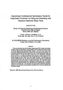
II. M ODELLING ISSUES The network structure is represented with a symmetric directed graph G = (V, A), where each node of set V corresponds to a router and the set of arcs A represents the connections between them, constituted by the transmission lines. The links between routers are taken to be full-duplex, with equal capacity in both directions. Each router is assumed to be composed by a chassis and a set of line cards. Each element of the routers can be switched on or off: each turned on device is characterized by a certain amount of energy consumption which is dependent on the quantity of processed traffic. As depicted in Figure 1, the power consumption of a router as function of the load follows therefore a kind of sawtooth wave, where each step corresponds to the activation of a line card, see [12], [13]. For a router with several line cards, a good approximation of the consumed power can be given by the linear power characteristic which connects power values W0 (chassis and one line card activated, but without traffic) and W f (chassis with all line cards switched on and maximum load, Γ, processed). In the proposed models a third power value, Ws , has been introduced: it represents the power consumption in standby condition (it is assumed that, for technical reasons, it is not possible to completely switch off a chassis, but only to put it in standby). The RES energy production was computed using suitable software products for photovoltaic plants design and simulation (like, e.g., PVsyst [14], [15]). The rebates can be given as

25

2013 IEEE INFOCOM Workshop on Communications and Control for Smart Energy Systems

Fig. 1. Schematic representation of measured (dashed line) and linearly fitted (continuous line) power characteristics of a router.

Fig. 3. Example of possible FIT (upper part of the figure) and generated earnings (lower part of the figure).

a percentage of the invested capital (r% ) or as a fixed amount of money (r f ). Suppose that the allowed expense is CII : in the first case, the total funding available to install the solar plants (named CI ) is given by CI = CII /(1 − 0.01r% ), while in the second case it is simply CI = CII +r f . The installation cost of a solar power plant has been modeled as a piecewise linear nonconvex function of the nominal installed power, as depicted in Figure 2. Each straight line is defined by the coefficient ai,k

ρi and Ai are, respectively, the nominal power and the area of each one of them. A¯ i is the maximum available area at i-th ¯ node. κ AAi ρi i , with κ > 1 is a therefore nominal power value greater than the maximum one installable at node i. θˆk and θ¯k are the values of the nominal power defining the beginning and the ending of each interval, which have to be different from nρi ∀n ∈ N, ∀i ∈ V , being N the set of natural numbers. It is easy to verify that Constraints (1) force νi,k + λi,k = 2 only in the intervals where the installed power mi ρi lies, while all the remaining intervals are characterized by νi,k + λi,k = 1. In this work implementation issues are not addressed: it is assumed that the routing strategies can be applied with small modifications to the network management platforms and that daily traffic profiles and electricity prices are both available.

III. M ATHEMATICAL PROGRAMMING FORMULATIONS Fig. 2. Example of price function used to model the costs of the solar power plants.

A. Cost-aware multi-period routing without PG (model ”R0 ”)

and bi,k , with i ∈ V and k ∈ P, being P the set of considered intervals (P = 1, 2, 3 in Figure 2). About FIT modeling, we took into account the fact that each unit of energy produced by the solar plants is remunerated with an amount of money ri,k that depends on the size of the PG [11] (and possibly on the location, i.e. on the node i), see Figure 3. We remark that the earnings generated by FIT as function of the PG size can have very irregular shapes. To handle the non-convex functions of FIT and costs, two binary auxiliary variables, λi,k and νi,k , are associated to each interval. Then, the following constraints are imposed   mi ρi − θˆk ≥ −θˆk (1 − νi,k )      mi ρi − θˆk ≤ (κ A¯ i ρi − θˆk )νi,k Ai , ¯k ≥ −θ¯k λi,k m ρ − θ  i i      mi ρi − θ¯k ≤ (κ A¯ i ρi − θˆk )(1 − λi,k ) Ai

First of all, a model for a basic cost-aware routing problem, called ”R0 ”, is presented. In this case, PG are not present in the network. The only task is to route demands so as to minimize operational costs in a multi-period setting taking into consideration the fact that electricity prices change in time and space. The solutions found using this model will be taken as references when assessing the impact of RES in the network management. The details of the formulation follow. a) Objective function: min ∑

∑ (eσi Wiσ )hσ

(2)

σ ∈S i∈V

where S is the set of periods in which the optimization horizon is divided, parameter eσi represents the electricity price at node i ∈ V in period σ ∈ S, parameter hσ is the duration of period σ ∈ S and the optimization variable Wiσ represents the power consumption of the i-th router in period σ ∈ S. The objective function therefore consists of the total operational costs of the network.

∀i ∈ V, ∀k ∈ P. (1) where mi is the number of modules installed at i-th node and

26

2013 IEEE INFOCOM Workshop on Communications and Control for Smart Energy Systems

b) Router power consumption constraints without PG: Wiσ ≥

horizon. g) Decision variable domains:

W f i −W0i d,σ d,σ ( ∑ ∑ qd,σ xd,σ xi, j ) j,i + ∑ ∑ q Γi ( j,i)∈A d∈D (i, j)∈A d∈D +W0i −W f i (1 − yσi ) Wiσ ≥ Wsi

∀i ∈ V, ∀σ ∈ S

∀i ∈ V, ∀σ ∈ S

uσi ∈ {0, 1}

(3) (4)

where D is the set of origin-destination demands, parameter qd,σ is the value of demand d ∈ D during period σ ∈ S. Router parameters W f i , W0i , Γi and Wsi are dependent on the node. Optimization routing variables xd,σ j,i are equal to 1 if the demand d ∈ D is routed on link (i, j) ∈ A during period σ ∈ S, and 0 otherwise. Optimization chassis status variables yσi are equal to 1 if a chassis i is switched on in period σ ∈ S, and 0 otherwise. Constraint (4) forces the power consumption of the i-th router to be greater or equal d,σ xd,σ ) to Wsi . Being (∑( j,i)∈A ∑d∈D qd,σ xd,σ j,i + ∑(i, j)∈A ∑d∈D q i, j the total traffic processed by the i-th router, when it is switched on (yσi = 1) Constraint (3) forces its power consumption to be above or on than the straight line between Wsi and W f i , while when the router is switched off (yσi = 0), Constraint (3) is always satisfied (because W f i > W0i > Wsi > 0). c) Arc capacity constraints:

∑ qd,σ xi,d,σj ≤ µi, j

∀(i, j) ∈ A, ∀σ ∈ S

∀i ∈ V, ∀σ ∈ S

(10)

Wiσ ≥ 0

∀i ∈ V, ∀σ ∈ S

(11)

xi,d,σ j yσi

∈ {0, 1}

∀(i, j) ∈ A, ∀σ ∈ S, ∀d ∈ D

(12)

∈ {0, 1}

∀i ∈ V, ∀σ ∈ S.

(13)

B. Cost-aware multi-period routing and PG installation (model ”RI ”) We recall that, when we solve this MILP model, the main goal is finding offline the optimal value of the optimization variable mi . a) Objective function: min ∑

∑ (eσi ζiσ − δiσ )hσ .

where the optimization power variable ζiσ and the optimization FIT variable δiσ represent, respectively, the amount of purchased non-renewable power and the earnings per unit of time at i-th node during period σ . The cost function consists in the total operational costs of the network. b) Router power consumption constraints with PG: Wiσ ≥ Wsi

(5)

d∈D

∀i ∈ V, ∀σ ∈ S

Wiσ ≤ Wsi +W f i yσi

where parameter µi, j represents the capacity of arc (i, j) ∈ A. d) Chassis capacity constraints:

Wiσ ≥

∀i ∈ V, ∀σ ∈ S

(15a) (15b)

W f i −W0i d,σ d,σ ( ∑ ∑ qd,σ xd,σ xi, j ) j,i + ∑ ∑ q Γi ( j,i)∈A d∈D (i, j)∈A d∈D

d,σ d,σ xi, j ≤ Γi yσi ∑ ∑ qd,σ xd,σ j,i + ∑ ∑ q ( j,i)∈A d∈D

(14)

σ ∈S i∈V

+W0i −W f i (1 − yσi )

∀i ∈ V, ∀σ ∈ S

(16a)

(i, j)∈A d∈D

∀i ∈ V, ∀σ ∈ S

(6)

Wiσ ≤

which impose the respect of the router capacity and force the chassis to be switched on (yσi = 1) when there is at least one demand incident to it. e) Flow conservation constraints (for single-path routing):  1 if i = sd ,   −1 if i = t d , ∑ xi,d,σj − ∑ xd,σ j,i =   (i, j)∈A ( j,i)∈A 0 otherwise. ∀i ∈ V, ∀σ ∈ S, ∀d ∈ D

+W0i +W f i (1 − yσi )

≥ yσi

− yσi −1

∑ uσi ≤ ηi

∀i ∈ V, ∀σ ∈ S ∀i ∈ V.

∀i ∈ V, ∀σ ∈ S. (16b)

Constraints (15b) and (16b) have to be added to force Wiσ to take the correct value. Indeed, where PG are present, this is not guaranteed by the fact that the objective function (14) is minimized. c, d, e, f) Constraints (5), (6), (7), (8), (9). g) Loops avoiding constraints:

(7)

d,σ xi,d,σ j + x j,i ≤ 1

where parameters sd and t d represent, respectively, the origin and destination of demand d ∈ D. f) Switching on restriction constraints: uσi

W f i −W0i d,σ d,σ ( ∑ ∑ qd,σ xd,σ xi, j ) j,i + ∑ ∑ q Γi ( j,i)∈A d∈D (i, j)∈A d∈D

∀i ∈ V, ∀d ∈ D, ∀(i, j) ∈ E, ∀σ ∈ S. (17) where E is the set of network edges (each couple of arcs corresponds to an edge). h) Single-passage constraints:

(8) (9)

∑

σ ∈S

xi,d,σ j ≤1

∀i ∈ V, ∀d ∈ D, ∀σ ∈ S.

(18)

(i, j)∈A

uσi

Constraints (8) guarantee that auxiliary binary variables take value 1 when router i is switched on in period σ , and 0 otherwise. Constraints (9) limit to ηi the number of switching on of the i-th router in the whole considered optimization

This constraint guarantees that the routing is performed without two or more passages of the same demand through the same router. Constraints (17) and (18) are needed because in presence of PG the energy could be available free of charges.

27

2013 IEEE INFOCOM Workshop on Communications and Control for Smart Energy Systems

i) Constraints on ζiσ : ζiσ ≥ Wiσ − mi pσi

∀i ∈ V, ∀σ ∈ S

b, c, d, e, f, g, h, i, j) Constraints (15a), (15b), (16a), (16b), (5), (6), (7), (17), (18), (8), (9), (19), (10), (11), (12), (13), (28).

(19)

pσi

where parameter represents the power production of a single photovoltaic module at i-th node during period σ . j) Maximum available area constraints: mi Ai ≤ A¯ i

∀i ∈ V

D. Remarks

(20)

Some remarks about the proposed MILP models are due.

k) Constraints (1) on auxiliary variables λi,k and νi,k . l) Single plants cost constraints:

•

ci ≥ (ai,k mi ρi + bi,k ) − C¯i (2 − νi,k − λi,k )

∀i ∈ V, ∀k ∈ P (21a) ∀i ∈ V, ∀k ∈ P (21b)

ci ≤ ai,k mi ρi + bi,k

•

where ci is the cost optimization variable equal to the price ¯ paid at i-th node for installing the PG and C¯i = κ(ai,1 AAi ρi i + bi,1 ), κ > 1. Given the shape of the price function, the term on the right side of Constraints (21a) is smaller than zero in all the intervals where νi,k + λi,k = 1. This means that the only active constraints are the one corresponding to the intervals in which νi,k + λi,k = 2. m) Total cost constraints:

∑ ci ≤ CI .

•

IV. C OMPUTATIONAL RESULTS

(22) A. Parameters used in the simulations

i∈V

n) Constraints on δiσ

≤ ri,k mi pσi

The models deal specifically with PG, but it is possible to apply them to any different kind of RES (all is needed is the value of pσi ). The minimization of the operational costs does not guarantee that a reduction in energy consumptions is achieved. To reach that target it is anyway sufficient adding the constraint ∑i∈V,σ ∈S Wiσ ≤ ε W¯ , with ε < 1, where W¯ is the total energy consumption of the network with the standard management strategy. The simplified model for the router, if needed, could be substituted with more accurate ones without having any conceptual difference.

δiσ :

+ r¯(2 − νi,k − λi,k )

∀i ∈ V, ∀k ∈ P, ∀σ ∈ S (23) ¯ where r¯ = maxi∈V,k∈P (ri,k AAii pi ) guarantees that only the constraints corresponding to the single interval where νi,k +λ i, k = 2 are activated. o) Decision variable domains (10), (11), (12), (13) and: ci ≥ 0

∀i ∈ V

(24)

mi ∈ N

∀i ∈ V

(25)

λi,k ∈ {0, 1}

∀i ∈ V, ∀k ∈ P

(26)

νi,k ∈ {0, 1}

∀i ∈ V, ∀k ∈ P

(27)

ζiσ δiσ

≥0

∀i ∈ V, ∀σ ∈ S

(28)

≥0

∀i ∈ V, ∀σ ∈ S.

(29)

1) Periods: the time horizon of one day has been divided into four periods, i.e. S = {1 (8 a.m. - 11 a.m.), 2 (11 a.m. - 7 p.m.), 3 (7 p.m. - 23 p.m.), 4 (23 p.m. - 8 a.m.) }. The instances for the MILP model RI have been solved considering only S = {1, 2}. 2) Networks topologies and communication devices parameters: for all the routers and arcs we set Wsi = 0.5 kW , W0i = 1.4 kW , W f i = 2 kW , and Γi = 50 Gigabit, ηi = 1 and µi, j = 5 Gigabit. As for the network topologies, we considered two examples, both taken from the largely used SND-Library [16]: nobelgermany (26 links and 17 nodes, see Figure 4) and dfn-bwin (45 links and 10 nodes, see Figure 5).

C. Cost-aware multi-period routing in presence of PG (model ”RR ”) In this case the position of PG (i.e., mi ), is known. The aim of the model is leading to the optimal online demand routing for networks where PG are installed. a) Objective function: min ∑

∑ (eσi ζiσ − ri mi pσi )hσ + ∑ ∑

σ ∈S i∈V˜

(eσi Wiσ )hσ

(30)

σ ∈S i∈V \V˜

where V˜ is the set that collects all the locations where PG are present. As before, the objective is to minimize the total cost due to the purchase of the non-renewable energy. As mi is now a known parameter, the size of each PG is fixed: thus, each ri is known as well.

Fig. 4.

28

nobel-germany network with 17 nodes and 26 links.

2013 IEEE INFOCOM Workshop on Communications and Control for Smart Energy Systems

Fig. 5.

and destination belonging to the first set. 2) The set of origin-destination demands is divided into two subsets and the demands of the first one have twice the magnitude of the second one. 3) The demands of the two subsets are initialized to 1.25 Gigabit to 0.625 Gigabit (1/4 and 1/8 of the links capacity). 4) A single-period version of R0 is used to route the demands. 5) If feasibility is found, the demands of the first subset are incremented by 0.625 Gigabit, while the demands of the second one are increased by 1.25 Gigabit. 6) The routing with R0 is performed again. 7) Points 4) and 5) are repeated until the problem stay feasible. The reference demands are the last ones for which R0 can be solved. 6) Considered benchmarks: The standard network management have consumptions dependent also (weakly) on the traffic. Being the traffic demands always smaller than their maximum possible values, we did not consider the reference power absorption of each router, W¯ i , always equal to W f i . Instead, presenting conservative results, according to [12], [13], we set W¯ i = 0.95W f i .

dfn-bwin network with 10 nodes and 45 links.

3) Photovoltaic modules data: modules SunPower SPR200-WHT-I/U with ρi = 0.2 kWp are considered. The installation instances were solved using the average energy production between March, 15th and October, 15th. For each considered network, the routing problems based on model RR was always solved in two different cases: in the first one, the output power of the photovoltaic modules has been set to the average production in May; in the second one, the month of September has been considered. We set C¯I = 50000 Euro, Ai = 2.8 m2 and A¯ i = 70 m2 for all the nodes. We chose P = {(−0.01, 10.01) − (10.01, 40.01)} (i.e., θˆ1 = −0.01,θˆ2 = 10.01, θ¯1 = 10.01, θ¯2 = 40.01) and ai,1 = 3000, ai,2 = 2800, bi,1 = 0 and bi,2 = 2000. As for the FIT we set ri,1 = 0.1836 and ri,2 = 0.1742. 4) Electricity prizes: the electricity prize is variable both with the period and with the location. To generate the data, a reference value, e∗ = 0.145 Euro/kW h, has been arbitrarily chosen. Then, for each of the four periods a nominal value e¯σi has been computed as e¯1i = 0.7e∗ , e¯2i = 0.9e∗ , e¯3i = 0.7e∗ and e¯4i = 0.5e∗ . e¯1i and e¯2i were used for RI , while for RR a random variation of ±20% was introduced to modify the nominal values. 5) Network demand generation: each period is characterized by a nominal demand and by a realistic demand. The nominal demand was generated as a fraction of a reference demand values di,∗ j , computed using a procedure explained later in this paragraph. Specifically the nominal demands related to the fourth periods are: d¯i,1 j = 0.6di,∗ j , d¯i,2 j = 0.75di,∗ j , d¯i,3 j = 0.3di,∗ j and d¯i,4 j = 0.1di,∗ j . d¯i,1 j and d¯i,2 j were used for RI . The realistic demands for RR were created randomly varying the nominal ones by ±20%. The reference demands di,∗ j were found with a method which aims at finding a realistic maximum feasible traffic level according to link capacities. The procedure is the following. 1) The set of nodes is splitted into two subsets: the first one contains the routers which can be origin or destination (or both) of demands, while the second one is constituted by the nodes that can only route traffic. The original set of the demands is then created selecting those having origin

B. R0 /RI /RR MILP models applied to networks nobel-germany and dfn-bwin The optimal solutions of RI model provided the optimal number of solar panels to be installed, shown in Table I. Node Berlin Bremen Dortmund Duesseldorf Essen Frankfurt Hamburg Hannover Karlsruhe Koeln Leipzig Mannheim Muenchen Norden Nuernberg Stuttgart Ulm

mi (nobel − germany) 4 0 0 0 0 24 0 0 0 0 0 0 20 7 0 21 7

mi (d f n − bwin) 12 24 0 0 0 0 0 23 0 24 -

TABLE I N UMBER OF PHOTOVOLTAIC PANELS TO BE INSTALLED AT EACH NODE OF nobel-germany AND dfn-bwin NETWORKS IN THE OPTIMAL SOLUTION TO RI MILP MODEL .

Figure 6 and in Figure 7 show the overall operating costs in the two networks obtained solving R0 and RR to optimality after having set mi to the values reported in Table I. The left y-axis is related to the real magnitude of the costs (in Euro), while the right y-axis gives their normalized value with respect to the reference case. R0 always allows to save more

29

2013 IEEE INFOCOM Workshop on Communications and Control for Smart Energy Systems

than 30% of the costs, with peak of 50% during the night. The introduction of PG, anyway, leads to a huge decrease in the costs during the first two periods, even generating earnings (negative costs) for the dfn-bwin network. Anyway, let us underline that these performances are possible thanks to an initial investment of 50000 Euro. Considering the month of September and the whole time horizon of one day, the costs obtained solving to optimality R0 model are 44.33 Euro and 27.27 Euro, respectively, for nobel-germany and dfn-bwin network, while the corresponding values resulting from the optimal solution to RR model are 27.48 Euro and 10.49 Euro. This means that installing the PG allows to reach savings equal to 16.85 Euro and 16.78 Euro in the two cases in September. Assuming an average of 13 − 15 Euro daily savings all year long, it takes approximately 10 years to refund the investment. For both nobel-germany and dfn-bwin network, the needed power lies always below 65% of the reference case, and during the night nearly half of the power can be saved.

aim at minimizing the operational costs. Temporal variation of the traffic demands and of the energy prices are considered, as well as constraints between different time periods. Since we assume that renewable energy sources can be located at some network nodes, we have addressed the problems of deciding where to install PG while respecting a maximum budget constraint, and of finding the optimal routing once PG have been properly placed. FIT and refunds are also considered and concave piecewise linear functions are used to model the cost for installing the PG. It has been found that considerable savings can be reached by adopting appropriate sleeping strategies, and that they can be significantly increased by installing photovoltaic generators in the network, in spite of initial investment. Future work includes the investigation of the case with different types of renewable energies and the extension of the proposed approach to more detailed models of routers. R EFERENCES [1] M. Gupta and S. Singh, “Greening of the internet,” in Proceedings of the 2003 conference on Applications, technologies, architectures, and protocols for computer communications. ACM, 2003, pp. 19–26. [2] A. Bianzino, C. Chaudet, D. Rossi, and J. Rougier, “A survey of green networking research,” Communications Surveys & Tutorials, IEEE. [3] R. Bolla, R. Bruschi, F. Davoli, and F. Cucchietti, “Energy efficiency in the future internet: a survey of existing approaches and trends in energy-aware fixed network infrastructures,” Communications Surveys & Tutorials, IEEE. [4] N. Vasi´c and D. Kosti´c, “Energy-aware traffic engineering,” in Proceedings of the 1st International Conference on Energy-Efficient Computing and Networking. ACM, 2010, pp. 169–178. [5] E. Amaldi, A. Capone, L. Gianoli, and L. Mascetti, “A MILP-based heuristic for energy-aware traffic engineering with shortest path routing,” in Network Optimization - 5th International Conference, INOC 2001, Lecture Notes in Computer Science, Vol. 6701. Springer, 2011, pp. 464–477. [6] S. Lee, P. Tseng, and A. Chen, “Link weight assignment and loop-free routing table update for link state routing protocols in energy-aware internet,” Future Generation Computer Systems, 2011. [7] Y. Zhang, M. Tornatore, P. Chowdhury, and B. Mukherjee, “Energy optimization in ip-over-wdm networks,” Optical Switching and Networking, 2011. [8] C. Cavdar, A. Yayimli, and L. Wosinska, “How to cut the electric bill in optical wdm networks with time-zones and time-of-use prices,” in Optical Communication (ECOC), 2011 37th European Conference and Exhibition on. IEEE, 2011, pp. 1–3. [9] X. Dong, T. El-Gorashi, and J. Elmirghani, “Ip over wdm networks employing renewable energy sources,” Lightwave Technology, Journal of. [10] ——, “Energy efficient optical networks with minimized non-renewable power consumption,” Journal of Networks. [11] T. Couture and Y. Gagnon, “An analysis of feed-in tariff remuneration models: Implications for renewable energy investment,” Energy Policy. [12] J. Chabarek, J. Sommers, P. Barford, C. Estan, D. Tsiang, and S. Wright, “Power awareness in network design and routing,” in INFOCOM 2008. The 27th Conference on Computer Communications. IEEE. Ieee, 2008, pp. 457–465. [13] P. Mahadevan, P. Sharma, S. Banerjee, and P. Ranganathan, “A power benchmarking framework for network devices,” NETWORKING 2009, pp. 795–808, 2009. [14] A. Mermoud, “Pvsyst: Software for the study and simulation of photovoltaic systems,” ISE, University of Geneva, www. pvsyst. com. [15] N. Van Der Borg and M. Jansen, “Energy loss due to shading in a bipv application,” in Photovoltaic Energy Conversion, 2003. Proceedings of 3rd World Conference on. [16] S. Orlowski, R. Wess¨aly, M. Pi´oro, and A. Tomaszewski, “Sndlib 1.0survivable network design library,” Networks.

Fig. 6. Overall costs of nobel-germany network obtained solving to optimality RR model in May (above) and September (below). Solid line (left y-axis): costs of the network with PG, in Euro. Dashed line (right y-axis): normalized costs with respect to the reference case. Dash-dot line (right yaxis): normalized costs of the network without PG managed using R0 model with respect to the reference case.

Fig. 7. Overall costs of dfn-bwin network obtained solving to optimality RR model in May (above) and September (below). Solid line (left y-axis): costs of the network with PG, in Euro. Dashed line (right y-axis): normalized costs with respect to the reference case. Dash-dot line (right y-axis): normalized costs of the network without PG managed using R0 model with respect to the reference case.

V. C ONCLUSIONS In this work, we have proposed mixed integer optimization models for smart communication network management which

30