Counting, Fanout, and the Complexity of Quantum ACC
arXiv:quant-ph/0106017v1 4 Jun 2001
Frederic Green Department of Mathematics and Computer Science Clark University, Worcester, MA 01610
[email protected] Steven Homer ∗ Computer Science Department Boston University, Boston, MA 02215
[email protected] Cristopher Moore † Computer Science Department University of New Mexico, Albuquerque NM 87131 and the Santa Fe Institute
[email protected] Christopher Pollett Department of Mathematics University of California, Los Angeles, CA
[email protected]
Abstract We propose definitions of QAC0 , the quantum analog of the classical class AC0 of constant-depth circuits with AND and OR gates of arbitrary fan-in, and QACC[q], the analog of the class ACC[q] where Modq gates are also allowed. We prove that parity or fanout allows us to construct quantum MODq gates in constant depth for any q, so QACC[2] = QACC. More generally, we show that for any q, p > 1, MODq is equivalent to MODp (up to constant depth). This implies that QAC0 with unbounded fanout gates, denoted QAC0wf , is the same as QACC[q] and QACC for all q. Since ACC[p] 6= ACC[q] whenever p and q are distinct primes, QACC[q] is strictly more powerful than its classical counterpart, as is QAC0 when fanout is allowed. This adds to the growing list of quantum complexity classes which are provably more powerful than their classical counterparts. ∗ †
Supported in part by the NSF under grant NSF-CCR-9988310 Supported in part by the NSF under grant NSF-PHY-0071139
We also develop techniques for proving upper bounds for QACC0 in terms of related language classes. We define classes of languages EQACC, NQACC and BQACCQ . We define a notion of log-planar QACC operators and show the appropriately restricted versions of EQACC and NQACC are contained in P/poly. We also define a notion of log-gate restricted QACC operators and show the appropriately restricted versions of EQACC and NQACC are contained in TC0 .
1
Introduction
Advances in quantum computation in the last decade have been among the most notable in theoretical computer science. This is due to the surprising improvements in the efficiency of solving several fundamental combinatorial problems using quantum mechanical methods in place of their classical counterparts. These advances led to considerable efforts in finding new efficient quantum algorithms for classical problems and in developing a complexity theory of quantum computation. While most of the original results in quantum computation were developed using quantum Turing machines, they can also be formulated in terms of quantum circuits, which yield a more natural model of quantum computation. For example, Shor [27] has shown that quantum circuits can factor integers more efficiently than any known classical algorithm for factoring. And quantum circuits have been shown (see Yao [33]) to provide a universal model for quantum computation. The theory of circuit complexity has long been an important branch of theoretical computer science. Shallow circuits correspond to parallel algorithms that can be performed in small amounts of time on a massively parallel computer with constant communication delays, and so circuit complexity can be thought of as a study of how to solve problems in parallel. In addition, some low-lying circuit classes have beautiful algebraic characterizations, e.g. [4, 5, 17]. In [18, 19], Moore and Nilsson suggested a definition of QNC, the quantum analog of the class NC of problems solvable by circuits with polylogarithmic depth and polynomial size [21]. Here, we will study quantum versions of some additional circuit classes. Recall the following definitions: 1. NCk consists of problems solvable by families of circuits of AND, OR, and NOT gates with depth O(logk n) and size polynomial in n, where n is the size of the input, and where the AND and OR gates have just two inputs each. 2. ACk is like NCk , but where we allow AND and OR gates with unbounded fan-in, i.e. arbitrary numbers of inputs, in each layer of the circuit. 3. ACCk [q] is like ACk , but where we also allow Modq gates with unbounded fan-in, where Modq (x1 , . . . , xn ) outputs 1 iff the sum of the inputs is not a multiple of q. 4. ACCk = ∪q ACCk [q]. 5. NC = ∪k NCk = ∪k ACk = ∪k ACCk . Then we have AC0 ⊂ ACC0 [2] ⊂ ACC0 ⊆ NC(1) ⊆ · · · ⊆ NC 2
In fact, these first two inclusions are known to be proper [2, 13, 22, 30]. Neither Majority nor Parity are in AC0 , while the latter is trivially in ACC0 [2]. In addition, ACC0 [p] and ACC0 [q] are known to be incomparable whenever p and q are distinct primes. Thus these classes give us some of the few strict inclusions known in computational complexity theory. However, for all anyone knows, ACC0 [6] could contain PP, NP, and the entire polynomial hierarchy! Quantum analogs of AC0 and ACC are defined and studied here. One central class that we examine is a quantum analog of AC0 that we denote QAC0wf . QAC0wf is the class of families of operators which can be built out of products of constantly many layers consisting of polynomialsized tensor products of one-qubit gates (analogous to NOT’s), Toffoli gates (analogous to AND’s and OR’s) and fan-out gates. The subscript “wf ” in the notation denotes “with fan-out.” The idea of fan-out in the quantum setting is subtle, as is made clear in Section 3 of this paper. The sub-class of QAC0wf that does not include fan-out gates is denoted simply QAC0 . An analog of ACC[q] (i.e., ACC circuit families only allowing Modq gates) is QACC[q], defined similarly to QAC0wf , but replacing the fan-out gates with quantum Modq gates (which we denote as MODq ). The class QACC is ∪q QACC[q]. In this paper, we prove a number of results about QAC and QACC, and address some definitional difficulties. We show that an ability to form a “cat state” with n qubits, or fan out a qubit into n copies in constant depth, is equivalent to being able to construct an n-ary parity gate in constant depth. We discuss how best to compare these circuit classes to classical ones. We prove the surprising result that, for any integer q > 1, QAC0wf = QACC[q] = QACC. This is in sharp contrast to the classical result of Smolensky [30] that says ACC0 [q] 6= ACC0 [p] for any pair of distinct primes q, p, which implies that for any prime p, AC0 ⊂ ACC0 [p] ⊂ ACC. This result shows that parity gates are as powerful as any other mod gates in QACC, and more generally, that any MODq gate is as good as any other, up to polynomial size and constant depth. Thus we conclude that QAC0wf , or, for any q, QACC[q], is strictly more powerful than ACC[q] and AC0 . We also develop methods for proving upper bounds for QACC. The definition of QACC immediately leads to a problem in this regard: QACC is a class of operators that only have a natural interpretation quantum mechanically. In order to clarify the relationship with classical computation we assign properties to QACC circuits based on measurements we can perform on them. In particular, we define several natural languages classes related to QACC. These language classes arise from considering a quantum circuit family in the class and specifying a condition on the expectation of observing a particular state after applying a circuit from the family to an input state. The condition might simply be that the expectation is non-zero, or that it is bounded away from zero by some constant, or that it is exactly equal to some constant. We call the language classes obtained by these conditions on the expectation NQACC, BQACC and EQACC, respectively. For example, the class NQACC corresponds to the case where x is in the language if the expectation of the observed state after applying the QACC operator is non-zero. This is analogous to the definition of the class NQP as defined in Adleman et al. [1] and discussed in Fenner et al. [12]. In this way we obtain natural classes of languages which correspond to those defined classically by families of small depth circuits. In these terms, for example, we can more succinctly and precisely express the statement “QACC[q] is strictly more powerful than ACC[q]” by writing ACC[q] ⊂ EQACC[q]. We desire upper bounds showing that these language classes are contained in classically defined circuit classes, thus delimiting the power of these quantum computations. In particular, we 3
believe that the languages arising in this way from our definitions are contained within TC0 , those problems computed by constant-depth threshold circuits. We have been unable to verify this, and in fact the only classical upper bound for these language classes that we know of is the very powerful counting class coC= P (see [12]). We do give some evidence for this proposed TC0 upper bound here and further provide some techniques which may prove useful in solving this problem. Our methods result in upper bounds for restricted QACC circuits. Roughly speaking, we show that QACC is no more powerful than P/poly provided that a layer of “wire-crossings” in the QACC operator can be written as log many compositions of Kronecker products of controlled-not gates. We call this class QACClog pl , where the “pl” is for this planarity condition. We show if one further restricts attention to the case where the number of multi-line gates (gates whose input is more than 1 qubit) is log-bounded then the circuits are no more powerful than TC0 . We call this class QACClog gates . These results hold for arbitrary complex amplitudes in the QACC circuits. log 0 In terms of our language classes, we show that NQACClog gates is in TC and NQACCpl is in P/poly. Although the proof uses some of the techniques developed by Fenner, Green, Homer and Pruim [12] and by Yamakami and Yao [31] to show that NQPC = coC= P, the small depth circuit case presents technical challenges not present in their setting. In particular, given a QACC operator built out of layers M1 , . . . , Mt and an input state |x, 0p(n) i, we must show that a TC0 circuit can keep track of the amplitudes of each possible resulting state as each layer is applied. After all layers have been applied, the TC0 circuit then needs to be able to check that the amplitude of one possible state is non-zero. Unfortunately, there could be exponentially many states with non-zero amplitudes after applying a layer. To handle this problem we introduce the idea of a “tensor-graph,” a new way to represent a collection of states. We can extract from these graphs (via TC0 or P/poly computations) whether the amplitude of any particular vector is non-zero. The exponential growth in the number of states is one of the primary obstacles to proving that all of NQACC is in TC0 (or even P/poly), and thus the tensor graph formalism represents a significant step towards such an upper bound. The reason the bounds apply only in the restricted cases is that although tensor graphs can represent any QACC operator, in the case of operators with layers that might do arbitrary permutations, the top-down approach we use to compute a desired amplitude from the graph no longer seems to work. We feel that it is likely that the amplitude of any vector in a tensor graph can be written as a polynomial product of a polynomial sum in some extension algebra of the ones we work with in this paper, in which case it is quite likely it can be evaluated in TC0 . Another important obstacle to obtaining a TC0 upper bound is that one needs to be able to add and multiply a polynomial number of complex amplitudes that may appear in a QACC computation. We solve this problem. It reduces to adding and multiplying polynomially many elements of a certain transcendental extension of the rational numbers. We show that in fact TC0 is closed under iterated addition and multiplication of such numbers (Lemma 5.1 below). This result is of independent interest, and our application of tensor-graphs and these closure properties of TC0 may prove useful in further investigations of small-depth quantum circuits. We now discuss the organization of the rest of this paper. Section 2 contains definitions for the quantum operator classes we will be considering as well as other background definitions. Section 3 shows the constant-depth quantum circuit equivalence of fan-out and parity gates. Section 4 establishes for arbitrary p and q the constant-depth quantum equivalence of Modp and Modq . Section 5 contains our upper bound results. Finally, the last section has a conclusion and some 4
open problems. Preliminary versions of these results appeared in [16] and [15].
2
Preliminaries
In this section we define the gates used as building blocks for our quantum circuits. Classes of operators built out of these gates are then defined. We define language classes that can be determined by these operators and give a couple of definitions from algebra. Lastly, some closure properties of TC0 are described. Definition 2.1 We define various quantum gates as follows: • By a one-qubit gate we mean an operator from the group U(2). • Let U =
u00 u01 u10 u11
!
∈ U(2). ∧m (U) is defined as: ∧0 (U) = U and for m > 0, ∧m (U) is
∧m (U)(|~x, yi) =
(
uy0 |~x, 0i + uy1 |~x, 1i if ∧m k=1 xk = 1 |~x, yi otherwise
!
01 • Let X = σx = . A Toffoli gate is a ∧m (X) gate for some m ≥ 0. A controlled-not 10 gate is a ∧1 (X) gate. • The Hadamard gate is the one-qubit gate H =
√1 2
!
1 1 . 1 −1
• An (m-)spaced controlled-not gate is an operator that maps |y1, . . . , ym , xi to |x ⊕ y1 , y2 . . . , ym , xi or |x, y1 , . . . , ym i to |x, y1 . . . , ym−1 , ym ⊕ xi • An (m-ary) fan out gate F is an operator that maps |y1, . . . , ym , xi to |x ⊕ y1 , . . . , x ⊕ ym , xi. • The classical Boolean Modq -function on n bits is defined so that Modq (x1 , . . . , xn ) = 1 iff Pn Pn i=1 xi 6≡ 0 mod q. We also define Modq,r (x1 , ..., xn ) to output 1 iff i=1 xi ≡ r mod q. A quantum MODq gate is an operator that maps |y1 , . . . , ym, xi to |y1 , . . . , ym , x ⊕ Modq (y1 , . . . , ym )i. A quantum MODq,r gate maps |y1 , . . . , ym, xi to |y1 , . . . , ym , x ⊕ Modq,r (y1 , . . . , ym )i. We write ¬MODq for MODq,0 . A parity gate is a MOD2 gate. Note that, since negation is built into the output (via the exclusive OR), it is easy to simulate negations using MODq,r gates (unlike the classical case). For example, by setting b = 1, we can compute ¬Modq,r . More generally, using one work bit, it is possible to simulate “¬MODq,r ,” defined so that, |x1 , ..., xn , bi 7→ |x1 , ..., xn , b ⊕ (¬Modq,r (x1 , ..., xn ))i using just MODq,r and a controlled-not gate. Thus MODq,r and ¬MODq,r are equivalent up to constant depth. Finally, observe that MOD−1 q,r = MODq,r . 5
π
=
θ
U
q
=
H
H
H
X
X
U
U
Figure 1. Our notation for n-ary Toffoli, controlled-U , and MODq gates, fanout gates, symmetric phase shift gates, and the Hadamard gate. On the top right, we show a useful identity between the controlled-not, the controlled π -shift, and the Hadamard gate. On the bottom right we show a controlled-U gate with one of its inputs negated by conjugation with X .
We will use the notation in Figure 1 for our various gates. As discussed in further detail in section 3 below, the no-cloning theorem of quantum mechanics makes it difficult to directly fan out qubits in constant depth (although constant fan-out in constant depth is no problem, since we can make multiple copies of the inputs). Thus it is necessary to define the operator F as in the above definition. Also, in the literature it is frequently the case that one says a given operator M on |y1 , . . . , ymi can be written as a tensor product of certain gates Mj . What is meant is that there is an permutation operator Π ( a map from |y1 , . . . , ym i to |yπ(1) , . . . , yπ(m) i for some permutation π) such that M|y1 , . . . ym i = Π ⊗nj Mj Π−1 |y1 , . . . ym i where the Mj ’s are our base gates, i.e. those gates for which no inherent ordering on the yi is assumed a priori, and ⊗ is the Kronecker product, which flattens a tensor product into a matrix with blocks indexed in a particular way. Since it is important to keep track of such details in our upper bounds proofs, we will always use Kronecker products of the form ⊗nj Mj without unspoken permutations. Nevertheless, being able to do permutation operators (not conjugation by a permutation) intuitively allows our circuits to simulate classical wire crossings. To handle permutations, we allow our circuits to have controlled-not layers. A controlled-not layer is a gate which performs, in one step, controlled-not’s between an arbitrary collection of disjoint pairs of lines in its domain. That is, it performs Π ⊗nj ∧1 (X)Π−1 for some permutation operator Π. It is easy to see [18] that any permutation can be written as a product of a constant number of controlled-not layers. We say a controlled-not layer is log-depth if it can be written as the composition of log many matrices each of which is the Kronecker product of identities and spaced controlled-not gates. M ⊗n is the n-fold Kronecker product of M with itself. Definition 2.2 QACk is the class of families {Fn }, where Fn is in U(2n+p(n) ), p a polynomial, and each Fn is writable as a product of O(logk n) layers, where a layer is a Kronecker product of one-qubit gates 6
and Toffoli gates or is a controlled-not layer. Also for all n the number of distinct types of one qubit gates used must be fixed. QACCk [q] is the same as QACk except we also allow MODq gates. QACCk = ∪q QACCk [q]. QACkwf is the same as QACk but we also allow fan-out gates.
QACC is defined as QACC0 and QACC[q] is defined as QACC0 [q]. QACClog pl is QACC restricted to log log-depth controlled not layers. QACCgates is QACC restricted so that the total number of multi-line gates in all layers is log-bounded. If C is one of the above classes and K ⊆ C, then CK are the families in C with coefficients restricted to K. Let {Fn } and {Gn }, Gn , Fn ∈ U(2n ) be families of operators. We say {Fn } is QAC0 reducible to {Gn } if there is a family {Rn }, Rn ∈ U(2n+p(n) ) of QAC0 operators augmented with operators from {Gn } such that for all n, x, y ∈ {0, 1}n , there is a setting of z1 , ..., zp(n) ∈ {0, 1} for which hy|Fn |xi = hy, z|Rn |x, zi. Operator families are QAC0 equivalent if they are QAC0 reducible to each other. If C1 and C2 are families of QAC0 equivalent operators, we write C1 = C2 . We refer to the zi ’s above as “work bits” (also called “ancillae” in [18]). Note that in proving QAC0 equivalence, the work bits must be returned to their original values in a computation so that they are disentangled from the rest of the circuit, and can be re-used by subsequent layers. It follows for any {Fn } ∈ QAC0 that Fn is writable as a product of finite number of layers. In an earlier paper, Moore [16] places no restriction on the number of distinct types of one-qubit gates used in a given family of operators. Here we restrict these so that the number of distinct amplitudes which appear in matrices in a layer is fixed with respect to n. This restriction arises implicitly in the quantum Turing machine case of the upper bounds proofs in Fenner, et al. [12] and Yamakami and Yao [31]. Also, it seems fairly natural since in the classical case one builds circuits using a fixed number of distinct gate types. Our classes here are, thus, more “uniform” than those defined earlier [16]. We now define language classes based on our classes of operator families. Definition 2.3 Let C be a class of families of U(2n+p(n) ) operators where p is a polynomial and n = |x|. 1. E·C is the class of languages L such that for some {Fn } ∈ C and {h~zn |} = {hzn,1 , . . . , zn,n+p(n)|} a family of states, m := |h~zn |Fn |x, 0p(n) i|2 is 1 or 0 and x ∈ L iff m = 1. 2. N·C is the class of languages L such that for some {Fn } ∈ C and {h~zn |} a family of states, x ∈ L iff |h~zn |Fn |x, 0p(n) i|2 > 0. 3. B·C is the class of languages L where for {Fn } ∈ C and {h~z|}, x ∈ L if |h~zn |Fn |x, 0p(n) i|2 > 3/4 and x 6∈ L if |h~zn |Fn |x, 0p(n) i|2 < 1/4 . It follows E·C ⊆ N·C and E·C ⊆ B·C. We frequently will omit the ‘·’ when writing a class, so E·QACC is written as EQACC. Let |Ψi := Fn |x, 0p(n) i. Notice that |h~zn |Fn |x, 0p(n) i|2 = hΨ|P|~zn i |Ψi, where P|~zn i is the projection matrix onto |~zn i. We could allow in our definitions measurements of up to polynomially many such projection observables and not affect our results below. However, 7
this would shift the burden of the computation in some sense away from the QACC operator and instead onto preparation of the observable. Next are some variations on familiar definitions from algebra. P
Definition 2.4 Let k > 0. A subset {βi }1≤i≤k of C is linearly independent if ki=1 ai βi 6= 0 for any (a1 , . . . , ak ) ∈ Qk − {~0k }. A set {βi }1≤i≤k is algebraically independent if the only p ∈ Q[x1 , . . . , xk ] with p(β1 , . . . , βk ) = 0 is the zero polynomial. We now briefly mention some closure properties of TC0 computable functions that are useful in 0 proving NQACClog gates ⊆ TC . For proofs of the statements in the next lemma see [28, 29, 10]. Lemma 2.5 (1) TC0 functions are closed under composition. (2) The following are TC0 computable: x + y, x −. y := x − y if x − y > 0 and 0 otherwise, |x| := ⌈log2 (x + 1)⌉, x · y, ⌊x/y⌋, 2min(i,p(|x|) , and cond(x, y, z) := y if x > 0 and z otherwise. (3) If f (i, x) is TC0 comPp(|x|) Qp(|x|) putable then k=0 f (k, x), k=0 f (k, x), ∀i ≤ p(|x|)(f (i, x) = 0), ∃i ≤ p(|x|)(f (i, x) = 0), and µi≤p(|x|)(f (i, x) = 0) := the least i such that f (i, x) = 0 and i ≤ p(|x|) or p(x) + 1 otherwise, are TC0 computable. We drop the min from the 2min(i,p(|x|)) when it is obvious a suitably large p(|x|) can be found. We define max(x, y) := cond(1 −. (y −. x)), x, y) and define maxi≤p(|x|) (f (i)) := µi≤p(|x|)(∀j ≤ p(|x|)(f (j) −. f (i) = 0) Using the above functions we describe a way to do sequence coding in TC0 . Let β|t| (x, w) := ⌊(w −. ⌊w/2(x+1)|t| ⌋ · 2(x+1)|t| )/2x|t| ⌋. The function β|t| is useful for block coding. Roughly, β|t| first gets rid of the bits after the (x+1)|t|th bit then chops off the low order x|t| bits. Let B = 2| max(x,y)| , so that B is longer than either x or y. Hence, we code pairs as hx, yi := (B+y)·2B+B+x, and projections . (0, β 1 . (0, β 1 as (w)1 := β⌊ 1 |w|⌋−1 ⌊ 2 |w|⌋ (0, w)) and (w)2 := β⌊ 12 |w|⌋−1 ⌊ 2 |w|⌋ (1, w)). We can encode a poly2 P 0 length, TC computable sequence of numbers hf (1), . . . , f (k)i as the pair h ki (f (i)2i·m), mi where m := |f (maxi (f (i)))| + 1. We then define the function which projects out the ith member of a sequence as β(i, w) := β(w)2 (i, w). We can code integers using the positive natural numbers by letting the negative integers be the odd natural numbers and the positive integers be the even natural numbers. TC0 can use the TC0 circuits for natural numbers to compute both the polynomial sum and polynomial product of a sequence of TC0 definable integers. It can also compute the rounded quotient of two such integers. For instance, to do a polynomial sum of integers, compute the natural number which is the sum of the positive numbers in the sum using cond and our natural number iterated addition circuit. Then compute the natural number which is the sum of the negative numbers in the sum. Use the subtraction circuit to subtract the smaller from the larger number and multiply by two. One is then added if the number should be negative. For products, we compute the product of the natural numbers which results by dividing each integer code by two and rounding down. We multiply the result by two. We then sum the number of terms in our product which were negative integers. If this number is odd we add one to the product we just calculated. Finally, division can be computed using the Taylor expansion of 1/x. 8
=
Figure 2. Two ways to make a cat state on n qubits. The circuit on the left uses only two-qubit gates and has depth log n. On the right, we define a “fanout gate” that simultaneously performs n controlled-nots from one input qubit.
3
Fanout, Cat States, and Parity
To make a shallow parallel circuit, it is often important to fan out one of the inputs into multiple copies. One of the differences between classical circuits and quantum ones as we have defined them here is that in classical circuits, we usually assume that we get arbitrary fanout for free, simply by splitting a wire into as many copies as we like. This is difficult in quantum circuits, since making an unentangled copy requires non-unitary, and in fact non-linear, processes: (α|0i + β|1i) ⊗ (α|0i + β|1i) = α2 |00i + αβ(|01i + |10i) + β 2 |11i has coefficients quadratic in α and β, so it cannot be derived from α|0i + β|1i using any linear operator, let alone a unitary one. This is one form of the so-called “no cloning” theorem. However, the controlled-not gate can be used to copy a qubit onto a work bit in the pure state |0i by making a non-destructive measurement: (α|0i + β|1i) ⊗ |0i → α|00i + β|11i Note that the final state is not a tensor product of two independent qubits, since the two qubits are completely entangled. This means that whatever we do to one copy, we do to the other. Except when the states are purely Boolean, we have to treat this kind of “fanout” more gingerly than we would in the classical case. By making n copies of a qubit in this sense, we can make a “cat state” α|000 · · · 0i+β|111 · · · 1i. Such states are useful in making quantum computation fault-tolerant (e.g. [9, 26]). We can do this in log n depth with controlled-not gates, as shown on the left-hand side of Figure 2. When preceded by a Hadamard gate on the top qubit, this circuit will map an initial state |0000i onto a cat state √12 (|0000i + |1111i). However, we will also consider circuits which can do this in a single layer, with a “fanout gate” that simultaneously copies a qubit onto n target qubits. This is simply the product of n controlled-not gates, as shown on the right-hand side of Figure 2. We now show that in quantum circuits, we can do fanout in constant depth if and only if we can construct a parity gate in constant depth. Proposition 3.1 In any class of quantum circuits that includes Hadamard and controlled-not gates, the following are equivalent: 9
= 2
=
H
H
H
H
H
H
H
H
=
H
H
H
H
H
H
H
H
Figure 3. The parity and fanout gates are conjugates of each other by a layer of Hadamard gates.
1. It is possible to map α|0i + β|1i and n − 1 work bits in the state |0i onto an n-qubit cat state α|000 · · · 0i + β|111 · · · 1i in constant depth. 2. The n-ary fanout gate on the right-hand side of Figure 2 can be implemented in constant depth with at most n − 1 additional work bits. 3. An n-ary parity or MOD2 gate as defined above can be implemented in constant depth with at most n − 1 additional work bits. Proof. First, note that (1) is a priori weaker than (2), since (1) only requires that an operator map |100 · · · 0i to |111 · · · 1i and |000 · · · 0i to itself. In fact, the two circuits shown in Figure 2 both do this, even though they differ on other initial states. To prove (2 ⇔ 3), we simply need to notice that the parity gate is a fanout gate going the other way conjugated by a layer of Hadamard gates, since parity is simply a product of controlled-nots with the same target qubit, and conjugating with H reverses the direction of a controlled-not. This is shown in Figure 3. Clearly the number of work bits used to perform either gate will be the same. (We prove this equivalence in greater detail and generality in Proposition 4.2 below.) To prove (1 ⇒ 3), we use a slightly more elaborate circuit shown in Figure 4. Here we use the identity shown in Figure 1 to convert the parity gate into a product of controlled π-shifts. Since these are diagonal, they can be parallelized as in [18] by copying the target qubit onto n − 1 work bits, and applying each one to a different copy. While we have drawn the circuit with two fanout gates, any gate that satisfies the conditions in (1), and its inverse after the π-shifts, will do. Finally, (2 ⇒ 1) is obvious.
This brings up an interesting issue. It is not clear that a QAC0 operator as we have defined QAC0 here can “simulate” any AC 0 circuit, since we are not allowing arbitrary fanout in each layer. An alternate definition, which we might call QAC with fanout or QAC0wf , would allow us to perform controlled-U gates or Toffoli gates in the same layer whenever they have different target qubits, even if their input qubits overlap. This seems reasonable, since these gates commute. Since we can fan out to n copies in log n layers as in Figure 2, we have QACk ⊆ QACkwf ⊆ QAC(k+1) . We can define QACCwf in the same way, and Proposition 3.1 implies that QACkwf = QACCkwf [2] = QACCk [2]. It is partly a matter of taste whether QAC0 or QAC0wf is a better analog of AC0 . However, fanout does seem possible in several proposed technologies for quantum computing. In an ion trap computer [8], vibrational modes can couple with all the atoms simultaneously, so we could apply a controlled-not from one atom to the “bus qubit” and then from the bus to the other n atoms. In bulk-spin NMR [14], we can activate the couplings from one atom to n others, and perform n controlled π-shifts simultaneously, which is equivalent to fanout with the target qubits 10
π
π π
=
π
=
π
π 2
H
H
H
H
0
0
0
0
Figure 4. The parity gate can also be written as a product of controlled π -shifts, with the target qubit conjugated by H . Since these are diagonal, we can parallelize them using any gate that can make a cat state .
conjugated with the Hadamard gate. Thus allowing fanout may in fact be the most reasonable model of constant-depth quantum circuits.
4
Constant Depth Equivalence of MODp and MODq Gates
As stated in the Introduction, in the classical case Modp and Modq gates are not easy to build from each other whenever p and q are relatively prime. In fact, to do it in constant depth requires a circuit of exponential size [30]. In this section, we will show this is not true in the quantum case. Specifically, we show that any MODq gate can be built in constant depth from any MODp gate, for any two numbers p and q. We start by showing that any MODq gate can be built from parity gates in constant depth. Proposition 4.1 In any circuit class containing n-ary parity gates and one-qubit gates, we can construct an n-ary MODq gate, with O(n log q) work bits, in depth depending only on q. Proof. Let k = ⌈log2 q⌉, and let M be a Boolean matrix on k qubits where the zero state has period q. For instance, if we write |xi as shorthand for |xk−1 · · · x1 x0 i where xi is the 2i digit of x’s binary expansion and 0 ≤ x < 2k , we can define M so that it permutes the |xi as follows: M|xi =
(
|(x + 1) mod qi |xi
if x < q if x ≥ q
Then if we start with k work bits in the state |0i and apply a controlled-M gate to them from each input, the state will differ from |0i on at least one qubit if and only if the number of true inputs is not a multiple of q. (Note that this controlled-M gate applies to k target qubits at once in an entangled way.) We can then apply an n-ary OR of these k qubits to the target qubit, i.e. a Toffoli gate with its inputs conjugated with X and its target qubit negated before or after the gate. We end by applying the inverse series of controlled-M † gates to return the k work bits to |0i. Now we use Proposition 4 of [18] to parallelize this set of controlled-M gates. We can convert them to diagonal gates by conjugating the k qubits with a unitary operator T , where T † DT = M 11
and D is diagonal. If we have a parity gate, we can fan out the k work bits to n copies each using Proposition 3.1. We can then simultaneously apply the n controlled-D gates from each input to the corresponding copy, and then uncopy them back. √ This is shown in Figure 5. For q = 3, for instance, M = 1
and D =
1 e2πi/3
010 0 0 1 100
,
3
T =
1
√1 3
1 e4πi/3 e2πi/3
1
e2πi/3 e4πi/3
1 1 1
,
.
e4πi/3 †
The operators T , T , and the controlled-D gate can be carried out in some finite depth by controlled-nots and one-qubit gates by the results of [3]. The total depth of our MODq gate is a function of these and so of q, but not of n. Finally, the number of work bits used is (n − 1)k = O(n log q) as promised.
To look more closely at the depth as a function of q, we note that using the methods of Reck et al. [23] and Barenco et al. [3], any operator on k qubits can be performed with O(k 3 4k ) two-qubit gates. Since k = ⌈log2 q⌉, this means that the depths of T , T † and the controlled-D gates are at most O(q 2 log3 q). Since we can construct MODq gates in constant depth, we have QACCk [q] ⊂ QACCk [2] for all q, so QACCk = QACCk [2]. By Proposition 3.1, these are both also equal to QACkwf . In particular, we have QAC0wf = QACC[2] = QACC while classically both equalities are strict inclusions. Note that allowing fanout immediately gives QACCwf [q] = QACC[2] = QACC for any q, but we will show below that including fanout explicitly is not necessary. We now show the converse QACC[2] ⊆ QACC[q] for any q, i.e. parity can be built from MODq for any q. This shows the constant depth equivalence of MODq gates for all q. Let q ∈ N, q ≥ 2 be fixed for the remainder of this section. Consider quantum states labeled by digits in D = {0, ..., q − 1}. By analogy with “qubit,” we refer to a state of the form, q−1 X
k=0
P
ck |ki
with k |ck |2 = 1 as a “qudigit.” We define three important operations on qudigits. The n-ary modular addition operator Mq acts as follows: Mq |x1 , ..., xn , bi = |x1 , ...xn , (b + x1 + ... + xn ) mod qi
We use the same graphical notation for Mq as we do for a MODq gate, but interpreting the lines as qudigits, as illustrated in Figure 6. Since Mq merely permutes the states, it is clear that it is unitary. Similarly, the n-ary unitary base q fanout operator Fq acts as, Fq |x1 , ...xn , bi = |(x1 + b) mod q, ...(xn + b) mod q, bi
We write F for F2 , since it is the “standard” fan-out gate introduced in Definition 2.1. Note that Mq−1 = Mqq−1 and Fq−1 = Fqq−1 . 12
=
0 0
}
0 M
M
M
M
q
M
M
0
log q
X
= M
M
M
T
T
D
D
D
D
T
T
= 0 0
0 D
0
0 0
0 D
0
Figure 5. Building a Modq gate. We choose a matrix M on k = ⌈log2 q⌉ qubits such that M q = 1, apply controlled-M gates from the n inputs to k work bits, apply an OR from these k qubits to the target qubit, and reverse the process to return the work bits to |0i. To parallelize this, we can diagonalize M by writing it as T † DT , fan the k qubits out into n copies each using Proposition 3.1, and apply controlled-D gates simultaneously from each input to a set of copies. The total depth depends on q but not on n.
13
. x1 . . u xn q (b + x1 + ... + xn ) mod q
x1 . . . xn
u
b
Figure 6. An Mq gate.
Finally, the Quantum Fourier Transform Hq (which generalizes the Hadamard transform H on qubits) acts on a single qudigit as, X 1 q−1 ζ ab |bi Hq |ai = √ q b=0 2πi
where ζ = e q is a primitive complex q th root of unity. It is easy to see that Hq is unitary, via Pq−1 aℓ the fact that ℓ=0 ζ = 0 iff a 6≡ 0 mod q. The first observation is that, analogous to parity and fanout for Boolean inputs, the operators Mq and Fq are “conjugates” in the following sense. This is a generalization of the equivalence of assertions (2) and (3) of Proposition 3.1. Proposition 4.2 Mq = (Hq⊗(n+1) )−1 Fq−1 Hq⊗(n+1) . Proof. We apply the operators Hq⊗(n+1) , Fq−1 , and (Hq⊗(n+1) )−1 in that order to the state |x1 , ..., xn , bi, and check that the result has the same effect as Mq . The operator Hq⊗(n+1) simply applies Hq to each of the n + 1 qudigits of |x1 , ..., xn , bi, which yields, 1 q
(n+1) 2
X q−1 X
y∈D n a=0
ζ x·y+ab|y1 , ..., yn , ai,
where y is a compact notation for y1 , ..., yn , and x · y denotes the above state yields, 1 q
(n+1) 2
X q−1 X
y∈D n
a=0
Pn
i=1
xi yi . Then applying Fq−1 to
ζ x·y+ab|(y1 − a) mod q, ..., (yn − a) mod q, ai.
By a change of variable, the above can be re-written as, 1 q
(n+1) 2
X q−1 X Pn
ζ
i=1
xi (yi +a)+ab
y∈D n a=0
14
|y1 , ..., yn , ai
Finally, applying (Hq⊗(n+1) )−1 to the above undoes the Fourier transform and puts the coefficient of a in the exponent into the last slot of the state. The result is, (Hq⊗(n+1) )−1 Fq−1 Hq⊗(n+1) |x1 , ..., xn , bi = |x1 , ..., xn , (b + x1 + ... + xn ) mod qi, which is exactly what Mq would yield. We now describe how the operators Mq , Fq and Hq can be modified to operate on registers consisting of qubits rather than qudigits. Firstly, we encode each digit using ⌈log q⌉ bits. Thus, for example, when q = 3, the basis states |0i, |1i and |2i are represented by the two-qubit registers |00i, |01i and |10i, respectively. Note that there remains one state (in the example, |11i) which does not correspond to any of the qudigits. In general, there will be 2⌈log q⌉ − q such “non-qudigit” states. Mq , Fq and Hq can now be defined to act on qubit registers, as follows. Consider a state |xi where x is a number represented as m bits (i.e., an m-qubit register). If m < ⌈log q⌉, then Hq leaves |xi unaffected. If 0 ≤ x ≤ q − 1 (where here we are identifying x with the number it √ Pq−1 xy ζ |yi. If x ≥ q, represents), then Hq acts exactly as one expects, namely, Hq |xi = (1/ q) y=0 again Hq leaves |xi unchanged. Since the resulting transformation is a direct sum of unit matrices and matrices of the form of Hq as it was originally set down, the result is a unitary transformation. Mq and Fq can be defined to operate similarly on m-qubit registers for any m: Break up the m bits into blocks of ⌈log q⌉ bits. If m is not divisible by ⌈log q⌉, then Mq and Fq do not affect the “remainder” block that contains fewer than ⌈log q⌉ bits. Likewise, in a quantum register |x1 , ..., xn i where each of the xi ’s (with the possible exception of xn ) are ⌈log q⌉-bit numbers, Mq and Fq operate on the blocks of bits x1 , ..., xn exactly as expected, except that there is no affect on the “non-qudigit” blocks (in which xi ≥ q), or on the (possibly) one remainder block for which |xn | < ⌈log q⌉. Since Mq and Fq operate exactly as they did originally on blocks representing qudigits, and like unity for non-qudigit or remainder blocks, it is clear that they remain unitary. Henceforth, Mq , Fq , and Hq should be understood to act on qubit registers as described above. Nevertheless, it will usually be convenient to think of them as acting on qudigit registers consisting of ⌈log q⌉ qubits in each. Lemma 4.3 Fq and Mq are QAC0 -equivalent. Proof. By Barenco et al. [3], any fixed dimension unitary matrix can be computed in fixed depth using one-qubit gates and controlled nots. Hence Hq can be computed in QAC0 , as can Hq⊗(n+1) . The result now follows immediately from Proposition 4.2. Lemma 4.4 MODq and Mq are QAC0 -equivalent. Proof. First note that ¬MODq and MODq,r are equivalent, since a MODq,r gate can be simulated by a ¬MODq gate with q − r extra inputs set to the constant 1. Since ¬MODq and MODq gates are equivalent, we can freely use MODq,r gates in place of MODq gates and vice versa. It is easy to see that, given an Mq gate, we can simulate a MODq gate. Applying Mq to n + 1 digits (represented as bits, but each digit only taking on the values 0 or 1) transforms, |x1 , ..., xn , 0i 7→ |x1 , ..., xn , ( 15
X i
xi ) mod qi.
(0)
u
(1)
u
(0)
u
x1
(1)
u u u
x1
e u e
0
x1
x1
0 x(0) n
. . . . . u.
≡
x(0) n
u
u u u (1) xn x(1) n e e u 0 0 q b b ⊕ mod(x)
u
qb, r
d Figure 7. A MOD 3,r circuit for r = 0. In the figure, mod(x) denotes notation on the right will be used as a shorthand for this circuit.
Mod3,r (x1 , ..., xn ). The
P
Now send the bits of the last block ( i xi mod q) to an n-ary OR gate with control bit b (see the proof of Proposition 4.1). The resulting output is exactly b ⊕ Modq (x1 , ..., xn ). The bits in the last block can be erased by reversing the Mq gate. This leaves only x1 , ..., xn , O(n) work bits, and the output b ⊕ Modq (x1 , ..., xn ). The converse (simulating Mq given MODq ) requires some more work. The first step is to show that MODq,0 can also determine if a sum of digits is divisible by q. Let x1 , ..., xn ∈ D be a set of (k) digits represented as ⌈log q⌉ bits each. For each i, let xi (0 ≤ k ≤ ⌈log q⌉ − 1) denote the bits of P⌈log q⌉−1 (k) k xi . Since the numerical value of xi is k=0 xi 2 , it follows that n X i=1
xi =
⌈log q⌉−1 n X X k=0
(k)
xi 2k .
i=1
The idea is to express this last sum in terms of a set of Boolean inputs that are fed into a (k) MODq,0 gate. To account for the factors 2k , each xi is fanned out 2k times before plugging it into the MODq,0 gate. Since k < ⌈log q⌉, this requires only constant depth and O(n) work bits (which of course are set back to 0 in the end by reversing the fanout). Thus, just using MODq,0 P and constant fanout, we can determine if ni=1 xi ≡ 0 mod q. More generally, we can determine if Pn d i=1 xi ≡ r mod q using just a MODq,r gate and constant fanout. Let MODq,r (x1 , ..., xn ) denote the resulting circuit, that determines if a sum of digits is congruent to r mod q. The construction d of MOD q,r (x1 , ..., xn ) is illustrated in Figure 7 for the case of q = 3. P d We can get the bits in the value of the sum ni=1 xi mod q using MOD q,r circuits. This is done, Pq−1 essentially, by implementing the relation x mod q = r=0 r · Modq,r (x). For each r, 0 ≤ r ≤ q − 1, we compute Modq,r (x1 , ..., xn ) (where now the xi ’s are digits). This can be done by applying d the MOD q,r circuits in series (for each r) to the same inputs, introducing a 0 work bit for each application, as illustrated in Figure 8. 16
x1
u
u
u
. . .
. . .
xn
u
0 0 0
b 0 q,
u
u
x1
xn
Modq,0(x1 , ..., xn ) Modq,1(x1 , ..., xn ) b 2 Modq,2 (x1 , ..., xn ) q,
qb, 1
d Figure 8. Applying MOD q,r circuits in series.
Let rk denote the k th bit of r. For each r and for each k, we take the AND of the output of d the MOD q,r with rk (again by applying the AND’s in series, which is still constant depth, but introduces q extra work inputs). Let ak,r denote the output of one of these AND’s. For each k, q−1 we OR together all the ak,r ’s, that is, compute ∨r=0 ak,r , again introducing a constant number of d work bits. Since only one of the r’s will give a non-zero output from MOD q,r , this collection of Pn OR gates outputs exactly the bits in the value of i=1 xi mod q. Call the resulting circuit C, and the sum it outputs S. Finally, to simulate Mq , we need to include the input digit b ∈ D. To do this, we apply a unitary transformation T to |S, bi that transforms it to |S, (b + S) mod qi. By Barenco, et al. [3] (as in the proof of Lemma 4.3), T can be computed in fixed depth using one-qubit gates and controlled NOT gates. Now using S and all the other work inputs, we reverse the computation of the circuit C, thus clearing the work inputs. This is illustrated in figure 9.
x1
. . .
xn 0 . C . . S 0 b
. . .
x1
xn . 0 . . S 0 (b + S) mod q C −1
T
Figure 9. Combining circuits to compute Mq .
The result is an output consisting of x1 , ..., xn , O(n) work bits, and (b + is the output of an Mq gate.
Pn
i=1
xi ) mod q, which
It is clear that we can fan out digits, and therefore bits, using an Fq gate (setting xi = 0 for 1 ≤ i ≤ n fans out n copies of b). It is slightly less obvious (but still straightforward) that, given an Fq gate, we can fully simulate an F gate. 17
Lemma 4.5 For any q > 2, F and Fq are QAC0 -equivalent. Proof. By the preceding lemmas, Fq and MODq are QAC0 -equivalent. By Proposition 4.1, MODq is QAC0 -reducible to F . Hence Fq is QAC0 -reducible to F . Conversely, arrange each block of ⌈log q⌉ input bits to an Fq gate as follows. For the control-bit block (which contains the bit we want to fan out), set all but the last bit to zero, and call the last bit b. Set all bits in the ith input-bit block to 0. Now the ith output of the Fq circuit is b, represented as ⌈log q⌉ bits with only one possibly nonzero bit. Send this last output bit b and the input bit xi to a controlled-NOT gate. The outputs of that gate are b and b ⊕ xi . Now apply Fq−1 to the bits that were the outputs of the Fq gate (which are all left unchanged by the controllednot’s). This returns all the b’s to 0 except for the control bit which is always unchanged. The outputs of the controlled-not’s give the desired b ⊕ xi . Thus the resulting circuit simulates F with O(n) work bits. Theorem 4.6 For any q ∈ N, q 6= 1, QACC = QACC[q]. Proof. By the preceding lemmas, fanout of bits is equivalent to the MODq function. Thus we can do fanout, and hence MOD2 , if we can do MODq . By the result of Proposition 4.1, we can do MODq if we can do fanout in constant depth. Hence QACC = QACC[2] ⊆ QACC[q].
To compare these results with classical circuits requires a little care. For any Boolean function φ with n inputs and m outputs, we can define a reversible version φ′ on n + m bits where φ′ (x, y) = (x, y ⊕ φ(x)) keeps the input x and XORs the output φ(x) with y. Then if φ has a circuit with depth d and width w, it is easy to construct a reversible circuit for φ′ of depth 2d − 1 where wd work bits start and end in the zero state. We do this by assigning a work bit to each gate in the original circuit, and replacing each gate with a reversible one that XORs that work bit with the output. Then we can erase the work bits by moving backward through the layers of the circuit. Then if we adopt the convention that a Boolean function with n inputs and m outputs is in a quantum circuit class if its reversible version is, we clearly have, for any k, ACk ⊆ QACkwf and ACCk ⊆ QACCk . Thus we have AC0 ⊂ ACC0 [2] ⊂ ACC0 ⊆ QAC0wf = QACC[q] = QACC showing that QAC0wf and QACC[2] are more powerful than AC0 and ACC0 [2] respectively. Interestingly, if QAC0 as we first defined it cannot do fanout, i.e. if QAC0 ⊂ QAC0wf , then in a sense it fails to include AC0 , since the fanout function from {0, 1} to {0, 1}n is trivially in AC0 . However, it is not clear whether it fails to include any AC0 functions with a one-bit output. On the other hand, if QAC0 can do fanout, it can also do parity and is greater than AC0 , so either way AC0 and QAC0 are different. We are indebted to Pascal Tesson for pointing this out.
5
Upper Bounds
log 0 0 In this section, we prove the upper bounds results NQACClog gates ⊆ TC , BQACCQ,gates ⊆ TC , log NQACClog pl ⊆ P/poly, and BQACCQ,pl ⊆ P/poly.
18
Suppose {Fn } and {zn } determine a language L in NQACC. Let Fn be the product of the layers U1 , . . . , Ut and E be the distinct entries of the matrices used in the Uj ’s. By our definition of QACC, the size of E is fixed with respect to n. We need a canonical way to write sums and products of elements in E to be able to check |h~z|U1 · · · Ut |x, 0p(n) i|2 > 0 with a TC0 function. To do this let A = {αi }1≤i≤m be a maximal algebraically independent subset of E. Let F = Q(A) and let B = {βi }0≤i 0, and we know ~x is in the language. In the BQACCQ case everything is a rational so P/poly can explicitly compute the magnitude of the amplitude and check if it is greater than 3/4. The TC0 result follows similarly from the TC0 part of Theorem 5.1. Finally, we note that some of the inclusions in the previous corollary can be strengthened if we assume that the circuit families are polynomial-time uniform and their coefficients polynomiallog time computable. In particular p-uniform NQACClog pl is contained in P and p-uniform NQACCgates is contained in p-uniform TC0 .
6
Discussion and Open Problems A number of open questions are suggested by our work. • Is QAC0 = QAC0wf ? That is, can the fanout gate be constructed in constant depth when each qubit can only act as an input to one gate in each layer? • Is QAC0wf = QTC0 ? That is, can the techniques used here be extended to construct quantum threshold gates in constant depth? • Is all of NQACC in TC0 or even P/poly? We conjecture that NQACC is in TC0 . As mentioned in the introduction, we have developed techniques that remove some of the important obstacles to proving this. • Are there any natural problems in NQACC that are not known to be in ACC? • What exactly is the complexity of the languages in EQACC, NQACC and BQACCQ ? We entertain two extreme possibilities. Recall that the class ACC can be computed by quasipolynomial size depth 3 threshold circuits [32]. It would be quite remarkable if EQACC could also be simulated in that manner. However, it is far from clear if any of the techniques used in the simulations of ACC (the Valiant-Vazirani lemma, composition of low-degree polynomials, modulus amplification via the Toda polynomials, etc.), which seem to be inherently irreversible, can be applied in the quantum setting. At the other extreme, it would be equally remarkable if NQACC and NQTC0 (or BQACCQ and NQTC0 ) coincide. Unfortunately, an optimal characterization of QACC language classes anywhere between those two extremes would probably require new (and probably difficult) proof techniques. • How hard are the fixed levels of QACC? While lower bounds for QACC itself seem impossible at present, it might be fruitful to study the limitations of small depth QACC circuits (depth 2, for example).
Acknowledgments: We thank Bill Gasarch for helpful comments and suggestions.
26
References [1] L. Adleman, J. DeMarrais, and M. Huang. Quantum computability. SIAM J. Computing 26 (1997) 1524–1540. [2] M. Ajtai. “Σ11 formulae on finite structures.” Ann. Pure Appl. Logic 24 (1983) 1–48. [3] A. Barenco, C. Bennett, R. Cleve, D.P. DiVincenzo, N. Margolus, P. Shor, T. Sleator, J.A. Smolin, and H. Weifurter, “Elementary gates for quantum computation.” Phys. Rev. A 52, pages 3457–3467, 1995. [4] D. A. Barrington, “Bounded-width polynomial-size branching programs recognize exactly those languages in NC1 .” J. Comput. System Sci. 38 (1989) 150–164. [5] M. Beaudry, P. McKenzie, P. P´eladeau, and D. Th´erien, “Circuits with monoidal gates.” Proc. Symposium on Theoretical Aspects of Computer Science (1993) 555–565. [6] C.H. Bennett, “Time/space trade-offs for reversible computation.” SIAM J. Computing 4(18) (1989) 766–776. [7] K. C. Chung and T. H. Yao, “On Lattices Admitting Unique Lagrange Interpolations.” SIAM Journal of Numerical Analysis 14 (1977) 735–743. [8] J.I. Cirac and P. Zoller, “Quantum computers with cold trapped ions.” Phys. Rev. Lett. 74 (1995) 4091–4094. [9] D.P. DiVincenzo and P.W. Shor, “Fault-tolerant error correction with efficient quantum codes.” quant-ph/9605031. [10] P. Clote, “On polynomial Size Frege Proofs of Certain Combinatorial Principles.” In P. Clote and J. Krajicek, editors, Arithmetic, Proof Theory, and Computational Complexity, Oxford (1993) 164–184. [11] L. Fortnow and J. Rogers, “Complexity Limitations on Quantum Computation.” Proc. 13th Conference on Computational Complexity (1998) 202–209. [12] S. Fenner, F. Green, S. Homer, and R. Pruim, “Quantum NP is hard for PH.” Royal Society of London A (1999) 455, pp 3953 - 3966. [13] M. Furst, J.B. Saxe, and M. Sipser, “Parity, circuits, and the polynomial-time hierarchy.” Math. Syst. Theory 17 (1984) 13–27. [14] N. Gershenfeld and I. Chuang, “Bulk spin resonance quantum computation.” Science 275 (1997) 350. [15] F. Green, S. Homer, and C. Pollett, “On the Complexity of Quantum ACC,” in Fifteenth Annual Conference on Computational Complexity Theory, IEEE Computer Society Press, (2000) 250-262. 27
[16] C. Moore, “Quantum Circuits: Fanout, Parity, and Counting.” quant-ph/9903046. [17] C. Moore, D. Th´erien, F. Lemieux, J. Berman, and A. Drisko , “Circuits and Expressions with Non-Associative Gates.” Journal of Computer and System Sciences 60 (2000) 368–394. [18] C. Moore and M. Nilsson, “Parallel quantum computation and quantum codes.” quantph/9808027, and to appear in SIAM J. Computing. [19] C. Moore and M. Nilsson, “Some notes on parallel quantum computation.” quantph/9804034. [20] R. A. Nicolaides, “On a class of finite elements generated by Lagrange interpolation.” SIAM Journal of Numerical Analysis 9 (1972) 177–199. [21] C.H. Papadimitriou, Computational Complexity. Addison-Wesley, 1994. [22] A.A. Razborov, “Lower bounds for the size of circuits of bounded depth with basis {&, ⊕}.” Math. Notes Acad. Sci. USSR 41(4) (1987) 333–338. [23] M. Reck, A. Zeilinger, H.J. Bernstein, and P. Bertani, “Experimental realization of any discrete unitary operator.” Phys. Rev. Lett. 73 (1994) 58-61. [24] M. Saks, “Randomization and derandomization in space-bounded computation.” Proc. 11th IEE Conference on Computational Complexity (1996) 128–149. [25] P.W. Shor, “Algorithms for quantum computation: discrete logarithms and factoring.” Proc. 35th IEEE Symposium on Foundations of Computer Science (1994) 124–134. [26] P.W. Shor, “Fault-tolerant quantum computation.” quant-ph/9605011. [27] P. W. Shor, “Polynomial-time algorithms for prime number factorization and discrete logarithms on a quantum computer.” SIAM J. Computing 26 (1997) 1484–1509. [28] K.-Y. Siu and V Rowchowdhury, “On optimal depth threshold circuits for multiplication and related problems.” SIAM J. Discrete Math. 7 (1994) 284–292. [29] K.-Y. Siu and J Bruck, “On the power of threshold circuits with small weights.” SIAM J. Discrete Math. 4 (1991) 423–435. [30] R. Smolensky, “Algebraic methods in the theory of lower bounds for Boolean circuit complexity.” Proc. 19th Annual ACM Symposium on Theory of Computing (1987) 77–82. [31] T. Yamakami and A.C. Yao, “NQPC = co-C= P .” To appear in Information Processing Letters. [32] A. C.-C. Yao, “On ACC and threshold circuits.” Proc. 31st IEEE Symposium on Foundations of Computer Science (1990) 619–627. [33] A. C.-C. Yao, “Quantum circuit complexity.” Proc. 34th IEEE Symposium on Foundations of Computer Science (1993) 352–361.
28