Descriptive Complexity of Optimization and Counting Problems

University of California Santa Cruz

Descriptive Complexity of Optimization and Counting Problems A dissertation submitted in partial satisfaction of the requirements for the degree of Doctor of Philosophy

in Computer and Information Sciences

by

Madhukar Narayan Thakur December 1992 The dissertation of Madhukar Narayan Thakur is approved: Phokion G. Kolaitis David Haussler Manfred K. Warmuth

Dean of Graduate Studies and Research

c by Copyright Madhukar Narayan Thakur 1992

iii

Dedicated to my parents Smt. Laxmi N. Thakur and Shri Narayan V. Thakur.

iv

Contents Dedication

iii

Abstract

viii

Acknowledgments

x

1. Introduction to Descriptive Complexity

1

2. Logic Preliminaries

4

I Optimization Problems

7

3. Introduction

8

3.1 Towards a structural theory of optimization problems : : : : : : : : : : : :

4. Classifying Optimization Problems

9

12

4.1 Computational Approaches : : : : : : : : : : : : : : : : : : : : : : : : : : :

13

4.2 The Logical De nability Approach : : : : : : : : : : : : : : : : : : : : : : :

21

5. Maximization Problems

24

5.1 Logical De nability of NP Max. Problems : : : : : : : : : : : : : : : : : : :

24

5.1.1 A characterization of MAX PB : : : : : : : : : : : : : : : : : : : :

24

5.1.2 Logical Hierarchy in MAXFO : : : : : : : : : : : : : : : : : : : : :

26

5.1.3 Approximation Properties of Subclasses of MAX FO : : : : : : : :

34

5.2 Logic and Feasible Solutions : : : : : : : : : : : : : : : : : : : : : : : : : : :

35

5.2.1 MAX PB and Feasible Solutions : : : : : : : : : : : : : : : : : : : :

35

5.2.2 Subclasses in MAX FFO : : : : : : : : : : : : : : : : : : : : : : : :

37

v

6. Minimization Problems

40

6.1 Logical De nability of NP Min. Problems : : : : : : : : : : : : : : : : : : :

40

6.1.1 A characterization of MIN PB : : : : : : : : : : : : : : : : : : : : :

40

6.1.2 Logical Hierarchy in MIN FO : : : : : : : : : : : : : : : : : : : : :

42

6.2 Approximation Properties of Subclasses of MIN FO : : : : : : : : : : : : :

48

6.3 Logic and Feasible Solutions : : : : : : : : : : : : : : : : : : : : : : : : : :

50

6.3.1 MIN PB and Feasible Solutions : : : : : : : : : : : : : : : : : : : :

51

6.3.2 Subclasses of MIN FFO : : : : : : : : : : : : : : : : : : : : : : : :

53

6.4 Approximation Properties of Subclasses of MIN FFO : : : : : : : : : : : :

56

6.4.1 The class MIN F+ 1 : : : : : : : : : : : : : : : : : : : : : : : : : : :

57

6.4.2 The class MIN F+ 2 : : : : : : : : : : : : : : : : : : : : : : : : : : :

62

7. On the Undecidability of Approximation Properties

69

8. Maximization Problems vs. Minimization Problems

73

9. Concluding Remarks

78

9.1 Discussion : : : : : : : : : : : : : : : : : : : : : : : : : : : : : : : : : : : : :

78

9.2 Non-polynomially bounded Optimization Problems : : : : : : : : : : : : : :

80

II Counting Problems

81

10.Introduction

82

11.Logical De nability of #P

86

11.1 Preliminaries : : : : : : : : : : : : : : : : : : : : : : : : : : : : : : : : : : :

86

11.2 A Descriptive Characterization of #P : : : : : : : : : : : : : : : : : : : : :

87

11.3 Logical Hierarchy in #P : : : : : : : : : : : : : : : : : : : : : : : : : : : :

90

vi

12.Computational Properties of Logically De ned Subclasses

95

12.1 Computational Properties of #1 : : : : : : : : : : : : : : : : : : : : : : : :

95

12.1.1 The class #0 : : : : : : : : : : : : : : : : : : : : : : : : : : : : : :

95

12.1.2 The class #1 : : : : : : : : : : : : : : : : : : : : : : : : : : : : : :

96

12.2 Good Computational Properties beyond #1 : : : : : : : : : : : : : : : : : 101 12.3 Undecidability of Some Computational Properties of #P Problems : : : : : 103

13.Discussion

106

References

107

A. De nitions of Max. and Min. Problems

111

B. De nitions of Counting Problems

118

vii

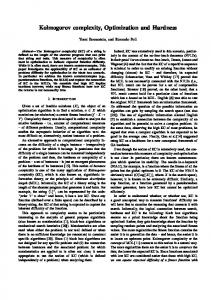
List of Figures 5.1 Classes of Maximization problems : : : : : : : : : : : : : : : : : : : : : : :

39

6.1 Classes of Minimization problems : : : : : : : : : : : : : : : : : : : : : : : :

56

Descriptive Complexity of Optimization and Counting Problems

Madhukar Narayan Thakur abstract

This thesis is about the descriptive complexity of two function classes, namely, NP optimization problems and #P counting problems. It is divided into two parts. In Part I we investigate NP optimization problems from a logical de nability standpoint. We show that the class of optimization problems whose optimum is de nable using rstorder formulae coincides with the class of polynomially bounded NP optimization problems on nite structures. Next, we analyze the relative expressive power of various classes of optimization problems in this framework. We introduce an alternate approach to the logical de nability of NP optimization problems by focusing on the expressibility of feasible solutions. We study the relationships between classes de ned in these two frameworks. We identify sucient syntactic conditions for approximability and isolate rich classes of approximable problems. Some of our results show that logical de nability has dierent implications for NP maximization problems than it has for NP minimization problems, in terms of both expressive power and approximation properties. Regarding the relationship between approximability and logical de nability, we show that, assuming P 6= NP, it is undecidable to tell if a given rst-order sentence de nes an approximable optimization problem.

Finally, we provide a machine-independent characterization of the NP =? co-NP problem in terms of logical expressibility of the MAX CLIQUE problem. We conclude Part I by discussing some future directions in this line of research. In Part II, we give a logic based framework for de ning counting problems and show that it exactly captures the problems in Valiant's counting class #P. We study the expressive power of the framework under natural syntactic restrictions and show that some of the subclasses so obtained contain problems in #P with interesting computational properties.

In particular, using syntactic conditions, we isolate a class of polynomial time computable #P problems, and also a class in which every problem is approximable by a polynomial time randomized algorithm. We show, under reasonable complexity theoretic assumptions, that it is undecidable to tell if a counting problem expressed in our framework is polynomial time computable or is approximable by a randomized polynomial time algorithm. This work sets the foundation for further study of the descriptive complexity of the class #P.

x

Acknowledgments I wish to thank my parents, my grandparents, and my brother for all the innumerable things that they have taught me and for their unwavering support and encouragement, especially during the Ph.D. program. I am specially grateful to my father for imparting to me his love of science and research. I am deeply indebted to my thesis advisor Professor Phokion Kolaitis who rekindled my latent interest in Logic in Computer Science. All that I have learned about the eld is due to his encouragement and guidance. I also thank him for suggesting the rst part of this thesis topic and working along with me in this research. Besides Logic, I have learned a lot from him, including research techniques and presentation of results in print and in seminars. Thank you, Phokion. Other members of my reading committee, Professors David Haussler and Manfred Warmuth, deserve thanks for reading this thesis in such a short time. It was Manfred Warmuth who introduced me to the interesting eld of Complexity Theory through his classes and many discussions. I am grateful to Professors Allen van Gelder and Nick Burgoyne who agreed to serve on my oral-exam committee. A part of the work involved in this thesis was initiated at the Tata Institute of Fundamental Research, Bombay. I wish to thank the faculty and sta of the Theoretical Computer Science Group of the institute for providing me with a good research environment one summer. I also extend my thanks to my collaborators, Sanjeev Saluja and K. V. Subrahmanyam, who were involved in the second part of this research. My colleagues and friends have provided much needed support through the course of this thesis. A special thanks goes to Neeta, whose support and love from halfway across the globe has done a lot to keep my morale high during the nal phases of this work. I thank Bala, Thomas, Vikram and Vikram, who provided me many thoughtful conversations, to KB for introducing me to the adventures of spelunking, during which some wild theorems were conjectured, to Phil, Cathi, and Shankar for all the enjoyable late night bridge games, and to Ravi and Ramanathan who provided encouragement and support from thousands of

xi miles away. I am also grateful to Sharon who edited the introductory chapters of this thesis and improved their readability. Numerous other people, by their pleasant distractions, made the rigors of the Ph.D. program less noticeable. Thank you Anil, Gunjan, Leena, Lisa, Max, Naim, Nicolo and Yoav. Finally, the sta of the CIS/CE boards at UCSC deserve my heartfelt thanks. They have been very helpful during my Ph.D. program.

1

1. Introduction to Descriptive Complexity Computer Science deals with solving problems on a computing device. Theoretical Computer Science has, over the years, tried to make precise the meaning of \problems" and \computing device". It has been accepted by computer scientists that Turing machines, or other equivalent devices, provide good models for studying problem-solving techniques, the precise speci cations of which are called algorithms. Computational complexity theory has traditionally focussed on the computational complexity of problems, which is the amount of resources, such as space or time, required by a computing device that solves the problem. A \problem" in this eld is often a language, de ned as a set of words over an alphabet. In this language setting, solving a problem amounts to answering YES or NO to the following question: Given a word w, is w in the language L? Computational models like Turing machines have been well studied as recognizers of languages (subsets of f0; 1g). This is especially true in computational complexity theory where resources like time and space can be de ned naturally using these machine models and the resource complexity of recognizing languages can be studied. More recently, mathematical logic has been used to study the complexity of recognizing the same languages. Logic provides a machine independent framework to study languages and the resources required to recognize them. In this approach, strings in f0; 1g are viewed as encodings of nite structures over an appropriate vocabulary, and formulae in a certain logic can be viewed as recognizers of languages in the following way. Let  be a vocabulary and let  be a sentence in a certain logic. One can associate with the formula  the language fe(A) 2 f0; 1g : A j= g where A is a nite structure over the vocabulary  and e(A) is an encoding of the structure A as a string in a natural way. Logical frameworks for de ning subsets of f0; 1g become much more interesting to a complexity theorist if there are appropriate logics that capture exactly the languages in the complexity classes that are otherwise de ned using computational machine models. These logical characterizations capture computational complexity without involving a model of

2 computation directly and suggest that logical expressibility of problems may determine their computational complexity. This is the direction taken by descriptive complexity theory [Imm89]. These studies began with the work of Fagin who provided a logical characterization of the class NP [Fag74]. A language L is in the class NP if and only if it is de nable by an existential second order sentence, i.e., if and only if there is a vocabulary  and a formula (S1 ;


; St) with predicate symbols amongst those in  SfS1 :


St g such that

e(A) 2 L () A j= (9S)(S); where A is a nite structure over the vocabulary  and e(A) is a string that encodes the structure A in a natural way. Another demonstration of such a close connection between computational and descriptive complexity was demonstrated by Immerman and Vardi [Imm86, Var82] who discovered a logical characterization of the complexity class P using xpoint logic. In addition to these results, researchers have provided logical characterization of many complexity classes; among these are the characterizations of uniform versions of the circuit class AC0 [BIS90], NLOGSPACE [Imm87b], and PSPACE [Imm87b]. The important results in this eld are surveyed in [Gur88, Imm87a, Imm89]. These are logical characterizations of language classes, or in other words, the above work studies how a decision problem can be de ned in a logical framework. With appropriate modi cations, the logical de nability framework can also be used to de ne classes of functions which map nite structures to natural numbers. Papadimitriou and Yannakakis [PY91] were the rst to use logic to study NP optimization problems. They showed that descriptive complexity of NP maximization problems has some bearing on the approximability of such problems in polynomial time. This set the logical de nability framework for further study of NP optimization problems and provided the motivation for study of descriptive complexity of function classes in general. In this thesis, we study the descriptive complexity of two dierent function classes, NP optimization problems and #P counting functions. This thesis is divided into two parts. We begin by presenting, in Chapter 2, some notation and background from logic. Then in

3 part I, we study the descriptive complexity of optimization problems arising from the class NP and in Part II, we study the descriptive complexity of #P, a counting class introduced by Valiant [Val79]. The results presented in Part I of this thesis have been arrived jointly with Phokion Kolaitis and are published in [KT90, KT91]. The results presented in Part II of the thesis dealing with counting problems have been arrived jointly with Sanjeev Saluja and K. V. Subrahmanyam and are published in [SST92].

4

2. Logic Preliminaries This chapter contains some basic de nitions from mathematical logic and a minimum amount of necessary background material from logical de nability theory. We give below brief de nitions of these terms and refer the reader to [End72] for a more rigorous treatment. De nition 2.1: [End72] A vocabulary (also known as a similarity type)  = fR~1;


; R~kg is a nite set of predicate symbols. Each predicate symbol R~i has a positive integer ri as

its designated arity. A structure A = (A; R1;


Rk ) over the vocabulary  consists of a set A, called the universe of A, and relations R1;


; Rk of arities r1;


rk on A, i.e., subsets of the Cartesian products Ar ; : : :; Ark respectively. A nite structure is a structure whose universe is a nite set. The size jAj of a nite structure A is the cardinality of its universe. 1

For example, a nite graph G = (V; E ) is a structure over a vocabulary with a single binary predicate E~ and a nite set of vertices V as the universe. In most cases either an NP decision problem is described directly as a problem on nite structures or it can be easily encoded by such a problem. For example, CLIQUE and VERTEX COVER are problems about nite graphs, while an instance I of SATISFIABILITY can be identi ed with a nite structure A(I ) = (X; C; P; N ), where X is the set of variables and clauses of I , the predicate C (x) expresses that x is a clause, and P (c; v) and N (c; v) are binary predicates expressing that a variable v occurs positively or negatively in a clause c. For the purpose of this thesis, we shall assume that the instances of an optimization problem (in Part I) and counting problem (in Part II) are given as nite structures over some vocabulary  . Since we will be using rst order logic extensively in this thesis, we give a brief de nition of this language.

De nition 2.2: A rst order language is a collection of formulae built up using predicate

symbols of a vocabulary  , the logical connectives ^; _; :; !, variables x1; x2; :::; y1 ; y2; :::; z1 ; z2; :::, quanti ers 9; 8 which range over the elements of the universe of a nite structure, and a built-in binary relation = which is always interpreted as equality. The reader is referred to [End72] for a thorough introduction on rst-order logic.

5

Notation: We shall use A; B; ::: to refer to nite structures and A; B; ::: to refer to the universe of these structures. We shall also use S, T to denote a nite sequence of predicate symbols, and w; x; y; z to denote a nite sequence of rst order variables. Every formula  of rst-order logic can be given semantics on structures over the vocabulary  . The predicate symbols of  are interpreted by the corresponding relations of the structure, the variables vi in the quanti ers (9vi ) and (8vi ), i  1, are interpreted as ranging over elements of the universe of the structure. The formula  becomes true or false on a structure A whenever a tuple of elements from the universe of the structure is assigned as interpretation to the sequence of the free variables of the formula, i.e., to those variables vi that do not always occur within the scope of a quanti er (9vi ) or (8vi ) in the formula (cf. [End72] for the precise de nitions). Let w be a nite sequences of variables. We shall write (w) to indicate that w is the sequence of the free variables of the formula . Finally, if A is a structure over the vocabulary  , then fw : A j= (w)g is the set of all tuples from the universe A of A for which the formula  becomes true (equivalently, the set of all tuples from A that satisfy ). For example, if G = (V; E ) is a graph, then fw : G j= (9y)(9z)(E~ (w; y) ^ E~ (w; z) ^ :(y = z))g is the set of all vertices of degree at least 2, i.e., the set of all vertices with at least two distinct neighbors. Notice that in order to simplify matters in the above expressions we mixed syntax with semantics by using the same notation for both a sequence of variables and a tuple of elements from the universe of the structure interpreting these variables. By the same token, from now on we shall take the liberty to use the same notation for both predicate symbols and relations on a structure interpreting these symbols. We trust that the reader is able to tell the dierence from the context.

6 Let S = (S1; : : :; Sm ) be a sequence of predicate symbols of arities s1 ; : : :; sm not in the vocabulary  . We write (w; S) to denote a formula of rst-order logic over the vocabulary  [ fS1; : : :; Smg having w as its free variables. If A = (A; R1; : : :; Rk ) is a structure over the vocabulary  and S1; : : :; Sm are relations on A of arities s1 ; : : :; sm respectively, then we write (A; S) to denote the expanded structure (A; R1; : : :; Rk ; S1; : : :; Sm). Thus,

fw : (A; S) j= (w; S)g denotes the set of all tuples from A for which the formula (w; S) becomes true on the expanded structure (A; S). For example, if G = (V; E ) is a graph and S is a subset of V , then fx : (G; S ) j= (8y )(E (x; y ) ! S (y ))g denotes the set of all vertices with the property that all their neighbors are in S . We also let fhw; Si : (A; S) j= (w; S)g denote the set of all pairs hw; Si, where w is a tuple from the universe A of A and S is a sequence of relations on the structure A, such that (w; S) becomes true on the expanded structure (A; S). In particular, fhSi : (A; S) j= (S)g is the set of all expansions of the structure A such that the expanded structure (A; S) satu es (S). For example, fhS i : G j= (8x)(8y)(S (x) ^ S (y):(x = y)) ! E (x; y)g is the set of all cliques in the graph G. De nition 2.3: A formula is in prenex normal form if and only if it contains no quanti ers, or it is in the form Q1 x1


Qk xk (x1;


xk ), where (x1;


xk ) is a quanti er-free formula, x1 ;


xk are (not necessarily distinct) variables, and Qi 2 f9; 8g, for i = 1;


; n. We denote by n ; n  1, the class of rst-order formulae in prenex normal form that have n ? 1 alternations of quanti ers and start with a block of existential quanti ers. For example, 1 is the collection of existential formulae, while 2 is the class of existentialuniversal formulae. Similarly, n , n  1, is the class of rst-order formulae in prenex normal form with n alternations of quanti ers, starting with a block of universal quanti ers. Thus, a 1 formula has universal quanti ers only, while 2 is the collection of universal-existential formulae. The class of quanti er-free formulae is denoted by 0 or by 0 .

7

Part I Optimization Problems

8

3. Introduction We study optimization problems arising from the class NP, a class of decision problems. To a large extent, optimization problems have provided motivation for the study of the class NP and the theory of NP-completeness. In fact, many natural NP-complete languages consist of decision problems that are derived from an optimization problem by imposing a bound on the objective function ([GJ79]). In return, the theory of NP-completeness has made it possible to prove a large set of optimization problems NP-hard. This means that nding an optimum solution for these problems is probably hard, i.e., cannot be done in polynomial time. In such a case, there are many approaches to solve an optimization problem. One approach is to nd probably optimal solutions. In this case, we seek fast, i.e., polynomial time, randomized algorithms. A randomized algorithm can toss coins as it runs and obtains a solution which is optimal with a very large probability. In general, it may not always obtain the best solution. The second approach is to use an algorithm that will always obtain an optimum solution at the cost of increasing its running time. On most inputs, the algorithm may execute fast, i.e., in polynomial time, but on some few inputs, it may take a long time to halt. In such cases, we seek algorithms that have fast average running time, where the average is taken w.r.t. some natural distribution over all inputs. A third approach is to sacri ce optimality of the solution to achieve polynomial running time. We seek polynomial time algorithms that will give us an approximate solution. This approach has lead to the study of approximation algorithms. In such a approach, a natural question to ask is, how good of an approximation can a given polynomial time algorithm achieve? Research in the eld of approximation algorithms has been in two directions. One led to a number of creative approximation algorithms for a variety of NP-hard optimization problems. The other direction led to classi cation of optimization problems. The motivation of this direction was to provide a robust theory of NP-optimization problems, that would classify optimization problems based on some structural similarities between them. We are

9 interested in such a structural theory. It would be very useful if such a theory also provided classes of problems with interesting computational properties, like the existence of \good" approximation algorithms for all the members of the class.

3.1 Towards a structural theory of optimization problems We have mentioned before that a problem in complexity theory often refers to the question of membership in a language. When naturally stated, optimization problems are not language problems. An optimization problem of the form, \given a graph G, what is the cardinality of the largest complete subgraph in G?", asks to evaluate a function from the set of all nite graphs into natural numbers. One can always disguise the function evaluation into a language problem under a suitable encoding. Given the impact of optimization theory on complexity theory and vice versa, it was natural to study optimization problems in the same framework as decision problems. For an optimization problem to be considered in this context, we must rst derive a language problem from it. There have been several attempts to classify optimization problems by classifying related language problems. Notable among these is the work of Krentel [Kre87], Wagner [Wag86], Leggett and Moore [LM81], Ausiello, and D'Atri and Protasi [ADP80]. (cf. [BJY89] for a comprehensive survey of the results in the area). We are interested in a structural theory of NP optimization problems that isolates interesting and natural classes of optimization problems with good approximation algorithms. However, the formalism of NP and complexity theory in general is ill-suited to the study of optimization problems from an approximation point of view. For an optimization problem to be considered in this context, we must rst derive a language problem from it. As a result of this rather awkward way of dealing with optimization problems in this framework, the theory of NP-completeness developed along a strikingly dierent path than the one taken by optimization theory. One of the reasons for the vast development of the theory of NP-completeness is the appropriate model of computation, namely, Turing machines and polynomial time reductions between problems. Turing

10 machines have a precise notion of \acceptance" of an input. This makes them good models of computation for studying decision problems. It is dicult to incorporate the notion of \approximate" solution in the Turing machine model of computation. The absence of a good model of computation for optimization problems has hindered the development of structural optimization theory on a par with structural complexity theory. Polynomial reducibility also seems to be an inappropriate notion of reduction between optimization problems. Although all known natural NPcomplete problems are polynomially isomorphic [BH77], their optimization counterparts have drastically dierent approximation properties. Even though the tools of complexity theory seem inappropriate to deal with classi cation of optimization problems, researchers have made some progress in classifying optimization problems so as to obtain classes of problems approximable by polynomial time algorithms. Notable is the work of Orponen and Manila [OM90], Crescenzi and Panconesi [CP88], and Paz and Moran [PM81]. The work in classifying optimization problems are attempts to answer some questions put forth by Johnson in 1974. In Johnson's words: [Joh74] \What is it that makes algorithms for dierent problems behave the same way? Is there some stronger kind of reducibility than the simple polynomial reducibility that will explain these results, or are they due to some structural similarity between the problems as we de ne them? And what other types of behavior and ways of analyzing and measuring it are possible?" Johnson's questions remained largely unanswered for a number of years. In 1988, Papadimitriou and Yannakakis [PY91] made the rst major, and quite successful, attempt to answer Johnson's questions about the structural similarity of some optimization problems based on their de nition. They brought a fresh perspective to this area by focusing on the logical de nability of optimization problems. This approach makes no explicit reference to Turing machines and provides a machine independent classi cation of optimization

11 problems. Later, Panconesi and Ranjan [PR90] showed the limited expressive nature of some of the classes of optimization problems de ned by Papadimitriou and Yannakakis. In Part I of this thesis, motivated by [PY91, PR90], we study optimization problems using logic. We study the logical de nability of NP maximization and minimization problems dierently. For minimization problems, we reveal a picture drastically dierent than the one for maximization problems. We show that logical de nability has dierent implications on maximization and minimization problems both in terms of expressive power and approximation properties. The logical framework used in [PY91, PR90] does not help us isolate classes of approximable minimization problems. Therefore, we modify the logical framework used in these papers and introduce a second framework and show the applicability of both these frameworks in de ning classes of approximable problems. Finally, for minimization problems, we identify syntactic conditions that imply approximability. This part of the thesis is organized as follows: In Chapter 4 we study, in more detail, some of the earlier work in classifying optimization problems. In Chapters 5 and 6, we study NP maximization and minimization problems respectively, their logical de nability and approximation properties. Having seen in these chapters that logic helps us de ne and study optimization problems, we ask: How far can logic help us in studying approximation behavior of optimization problems? As an answer to this question, we show in Chapter 7 that it is an undecidable problem to say whether or not an optimization problem, stated in a logical framework, is approximable. In Chapter 8 we study the relationship between maximization and minimization problems and provide a purely logical characterization of the NP =? coNPproblem. Finally, in Chapter 9, we end Part I by discussing some directions for future work.

12

4. Classifying Optimization Problems In this chapter, we review some of the earlier approaches to the study of NP optimization problems. The approaches can be classi ed into two types. Those which study the nature of optimization problems by studying the structure and computational complexity of associated language problems, and those which study the logical de nability of these optimization problems. This thesis takes the second approach. In Section 4.1, we review some of the earlier work in classifying optimization problems using the computational approach. In Section 4.2 we review the recent work in using the logical de nability approach to classify optimization problems and lay the foundation for our work in this area. In the review of previous work, sometimes we use a notation dierent from that used by the original researchers; our aim in doing so is to use a common notation, as far as possible, to integrate the results of previous researchers and our own. We begin by de ning an NP optimization problem.

De nition 4.1: An NP optimization problem is a tuple Q = (IQ; FQ; fQ; optQ) such that  IQ is the set of input instances. It is assumed that IQ can be recognized in polynomial time.

 FQ(I ) is the set of feasible solutions for the input I .  fQ is a polynomial time computable function, called the objective function. It takes positive integer values and is de ned on pairs (I; T ), where I is an input instance and T is a feasible solution of I .  optQ is one of the two functions de ned below, from IQ into positive integers. optQ(I ) = max f (I; T ) or optQ(I ) = min f (I; T ): T Q T Q In the former case, we say Q is a maximization problem and in the later case we say Q is a minimization problem.

 The following decision problem is in NP : Given I 2 IQ and an integer k, does there exist a feasible solution T 2 FQ (I ) such that fQ (I; T )  k, for a maximization

13 problem Q (or, fQ (I; T )  k, for a minimization problem Q)? We shall call this the standard decision problem associated with the optimization problem Q. Let NPOpt denote the class of all NP optimization problems. An optimization problem Q is said to be NP-hard if the standard decision problem associated with Q is NP-complete. The above de nition is a variation of the de nition given by [PR90] and is broad enough to encompass every known optimization problem arising in NP-completeness. For example, the MAX CLIQUE1 optimization problem has as input space the set of all nite undirected graphs, the set of feasible solutions of a given graph G is the set of all complete subgraphs of G, and the objective function is the number of vertices in the complete subgraph.

De nition 4.2: An NP optimization problem Q is said to be polynomially bounded if there

is a polynomial p such that

optQ (I )  p(jI j) for all I 2 IQ; where jI j is the length of the input I . Let MAX PB (MIN PB) denote the class of all polynomially bounded NP maximization (minimization) problems. MAX CLIQUE, MAX SAT, MIN VERTEX COVER, and MIN DOMINATING SET are examples of polynomially bounded NP optimization problems. On the other hand, MIN TSP, KNAPSACK are not polynomially bounded optimization problems.

4.1 Computational Approaches Leggett and Moore [LM81] were amongst the rst to study optimization problems by studying the complexity of determining membership in a related set. Corresponding to an optimization problem Q = (IQ ; FQ; fQ ; optQ), they de ne the set EXACT(Q)2 as follows: EXACT(Q) = f(I; k) : I 2 IQ and optQ (I ) = kg: 1 2

Appendix A contains precise de nitions of this and other optimization problems used in this thesis. Leggett and Moore called this OPT(Q).

14 The membership question in this set can be equivalently stated as, given an instance I and an integer k, is the optimum value of the objective function, on input I , equal to k? Leggett and Moore prove the following result for polynomially bounded problems. Theorem 4.1: Let Q be a polynomially bounded NP-hard optimization problem. If NP 6= coNP, EXACT(Q) is a proper-PNP problem. This means, if NP 6= coNP, EXACT(Q) 62 NP [ coNP : The proofs involved in their work do not use the full power of the class PNP . The essence of their results is that, to solve an NP-hard optimization problem exactly, we have to solve two problems, an NP-complete problem and a coNP-complete problem. Papadimitriou and Yannakakis [PY84] (cf. also [PW88]) studied the class of such problems and called it the class DP . De nition 4.3: The class DP is de ned as fL1 \ L2 : L1 2 NP ; L2 2 coNP g: Papadimitriou and Yannakakis [PY84] show that if Q is an NP-hard optimization problem, then EXACT(Q) is a language complete for DP . This result subsumes some of the results of Leggett and Moore. Papadimitriou and Yannakakis' work on the class DP generated interest in the closure of NP under boolean operations and the natural optimization problems that lie in the dierent classes so obtained. Prominent in this area is the work of Wagner [Wag86] who studied the related language problems and placed them in the Boolean Hierarchy. The Boolean Hierarchy was introduced and investigated independently in [CH86, WW86]. The simplest question one can ask about an optimization problem Q is the standard decision problem, namely, given I 2 IQ and an integer k, is optQ (I )  k (or is optQ (I )  k)? Wagner studied the complexity of more complicated questions about maxima and minima of optimization problems. In particular, he studied the following languages related to an NP optimization problem Q.

De nition 4.4:

Qk = f(I; a1;


ak ) : I 2 IQ; a1;


ak 2 N and optQ (I ) 2 fa1;


ak gg; k  1: Qodd = fI : I 2 IQ and optQ(I ) is oddg:

15 Wagner was interested in classifying the languages Qk and Qodd corresponding to problems Q which are polynomially bounded, which are polynomially invertible, and which are neither polynomially bounded nor polynomially invertible. He de ned an optimization problem to be polynomially invertible as follows:

De nition 4.5: An optimization problem Q is polynomially invertible if the mapping (I; n) ! fT : T 2 FQ (I ) and fQ (I; T ) = ng; for all I 2 IQ ; n 2 N is polynomial time computable. MAX SATISFYING ASSIGNMENT is an example of a polynomially invertible optimization problem. On the other hand, MIN TSP, and MAX CLIQUE are not polynomially invertible. Wagner proved the following theorem.

Theorem 4.2:

 If Q is a polynomially bounded optimization problem, then Qk is NP NP Wk complete for C2NP k and Qodd is complete for Pbf , where C2k = i=1 (NP ^ coNP) and P PNP bf is the closure of NP w.r.t polynomial time boolean formula reducibility (bf ). Note that the class C2NP has been called DP in [PY84].

 If Q is a polynomially invertible optimization problem, then Qk is complete for the class coNPand Qodd is complete for the class PNP .  Finally, if Q is neither polynomially bounded nor polynomially invertible, then Qk is NP complete for the class C2NP k and Qodd is complete for the class P . With this work, Wagner provided insight into the computational complexity of various decision problems arising from an optimization problem. Wagner's work and that of others cited above studies optimization problems by classifying the complexity of some related decision problems. Krentel, on the other hand, approached the complexity of optimization problems by studying the complexity of function classes directly. The main focus of his work was to exhibit a deeper structure among NP optimization problems. Krentel gave an alternate, but equivalent, de nition of an NP maximization (minimization) problem based on polynomial time non-deterministic machines, which write an integer value on every accepting path and the output of the

16 machine is the maximum (minimum) integer written. He called them Metric Turing machines. The functions computed by such machines are exactly the class of NP optimization problems de ned above. Krentel de ned subclasses of NPOpt3 as follows:

De nition 4.6: We say Q is in the class NPOpt[z(n)], if optQ (I ) is written in binary

using z (n) bits where n = jI j. In this notation, NPOpt[O(log n)] is precisely the class of polynomially bounded NP optimization problems. Note that NPOpt = NPOpt[nO(1)].

Krentel studied a suitable notion of polynomial reducibilities between functions in NPOpt. He called it a metric reduction, but it turns out that this is equivalent to a one-truth-table reduction.

De nition 4.7: Let Q; R 2 NPOpt. We say Q is metric reducible to R if there exist two

polynomially computable functions t1 : IQ ! IR and t2 : (IR  N ) ! IQ , such that optQ (I ) = t2 (I; optR(t1 (I ))) for all I 2 IQ . Using this notion of metric reduction, Krentel showed many problems complete for the classes NPOpt and for NPOpt[O(log n)].

Theorem 4.3: MAX WEIGHTED SATISFIABILITY, MIN TSP, KNAPSACK, 0-1 INTEGER PROGRAMMING are complete for NPOpt under metric reductions. MAX SAT, MAX CLIQUE, MIN COLORING, and LONGEST CYCLE are complete for NPOpt[O(log n)] under metric reductions. Such results help separate optimization problems by directly separating their functional versions. The proofs of completeness of most of the above problems are straightforward variations of those used to prove that the associated standard decision problem is NP complete. With an aim of \quantifying the extent of NP completeness" present in an NP optimization problem Q, Krentel raised the question, how many queries to an NP oracle does it take to solve an NP optimization problem Q in polynomial time? In the process of answering this question, he related NPOpt to FPSAT which is de ned as follows. We give the de nitions in the context of optimization problems. 3

Krentel called the class OptP

17

De nition 4.8: An optimization problem Q is in FPSAT if optQ is computable in

polynomial time given access to an oracle for SATISFIABILITY. We say Q is in FPSAT [z (n)] if Q 2 FPSAT and optQ is computable using at most z (n) queries on inputs of length n. Krentel's main result is that a problem complete for NPOpt[O(z (n))] via metric reductions is also complete for FPSAT [z (n)]: Thus MAX WEIGHTED SATISFIABILITY, MIN TSP, KNAPSACK, 0-1 INTEGER PROGRAMMING are all complete for FPSAT and MAX SAT, MAX CLIQUE, MIN COLORING, and LONGEST CYCLE are complete for FPSAT [O(log n)]. He further classi ed problems within FPSAT and dierentiated between using O(log n) and nO(1) queries to a SAT oracle. He proved the following theorem.

Theorem 4.4: If FPSAT[O(log n)] = FPSAT [nO(1)] then P = NP.

As a corollary, it follows that, unless P = NP, there is no metric reduction from MIN TSP to MAX CLIQUE and, therefore, TSP is strictly harder to solve (optimally) than MAX CLIQUE. He also proved the following theorem to make a ner distinction between optimization problems based on the number of queries to a SAT oracle required to compute the optimum.

Theorem 4.5: Let f (n); g(n) be non-decreasing functions such that 1n 7! 1f (n), 1n 7! 1g(n) are polynomial time computable, for all n, f (n) < g (n), and f (n) < 21 log n: If FPSAT [f (n)] = FPSAT [g (n)] then P = NP. This separates the complexity of problems like BIN PACKING and MAX CLIQUE. This is because, MAX CLIQUE is complete for FPSAT [O(log n)], but BIN PACKING can be solved in polynomial time with 2 log log n + O(1) queries to SAT [KK82]. The work described above studies the diculty of solving various optimization problems and related language problems exactly. It was aimed at providing structural properties of language classes related to the maximum/minimum solutions of optimization problems and of the function classes directly. However, it hardly addresses the existence of polynomial time approximation algorithms. We rst de ne an approximation algorithm and discuss some past work in this area.

18

De nition 4.9: Let g(n) be a function from positive integers to positive reals. We say that

an algorithm is a g (n)-approximation algorithm for an optimization problem Q if, given an instance I of Q, the algorithm produces a feasible solution T such that

8 > < g(jI j)  > :

f (I;T ) optQ(I )

if Q is a minimization problem

optQ(I ) f (I;T )

if Q is a maximization problem;

where jI j denotes the size of the instance I . We say that an optimization problem is g(n)-approximable if there is a polynomial time g(n)-approximation algorithm for it. We say that an optimization problem is O(g (n))-approximable if it is cg (n)-approximable for some constant c > 0. An optimization problem is constant-approximable, if it is g (n)approximable for some constant function g (n) = c, i.e., if it is O(1)-approximable. Similarly, an optimization problem is log-approximable if it is O(logn)-approximable. For every   0, if there is a (1 + )-approximation algorithm A ; then Q is said to have a polynomial time approximation scheme (PTAS). Further, if the running time of A is bounded by a polynomial in 1=, then Q is said to have a fully polynomial time approximation scheme (FPTAS). The theory of NP-completeness is not ne enough a sieve to separate optimization problems according to their approximability. A variety of optimization problems, whose decision versions are NP-complete have vastly dierent approximation behavior. They range from being non-approximable on one extreme to having FPTAS. For example, MAX CLIQUE is not constant approximable [AS92, ALM+ 92] unless P = NP. On the other hand a large number of optimization problems like MAX SAT, MAX CUT, MIN VERTEX COVER, and MIN TSP with weights f1, 2g are constant-approximable [PS82]. On a more positive note, the MAX INDEPENDENT SET problem restricted to planar graphs has a PTAS [Bak83] and the KNAPSACK problem has a fully polynomial time approximation scheme [IK75]. On the other hand, no PTAS exists for MAX 3SAT, MAX CUT, MIN VERTEX COVER, unless P = NP [ALM+ 92]. One of the rst attempts made to study optimization problems with an aim of deriving necessary and sucient conditions for their approximability, was made by Paz

19 and Moran [PM81]. They observed that for many NP optimization problems Q, for every constant k, there is a polynomial time algorithm to decide if optQ (I )  k. They called such problems simple. Paz and Moran showed the following conditions to be necessary and sucient for the existence of a PTAS for an NP maximization problem.

Theorem 4.6: An NP maximization problem has a PTAS if and only if  Q is simple  There is a positive constant h such that for every instance I 2 IQ and every positive integer c O  optQc (I ) ? B(I; c)  h;

where B : IQ  N ! N and B (I; n) be computable in time polynomial in jI j and optQ(I ).

An analogous result holds for minimization problems too. Such necessary and sucient conditions are not very interesting as they are themselves stated, implicitly, in terms of approximate solutions. Orponen and Mannila [OM90] studied minimization problems and reductions between such problems. These reductions have the property that they preserve approximability within a constant factor between optimization problems We use here a variant of these reductions introduced by Crescenzi and Panconesi [CP89].

De nition 4.10: [CP89] Let Q and R be two NP optimization problems. An

approximabilty preserving reduction (or, A-reduction) from Q to R is a triple  = (t1 ; t2; c) for which the following hold:

 t1 : IQ ! IR and t2 : IR  FR ! FQ are polynomially computable functions.  If T is a g(n)-approximate solution for an instance t1(I ) of R, then t2(I; T ) is an O(g(n))-approximate solution for Q. If there is an A-reduction form Q to R, then we say that Q is A-reducible to R and we write Q A R. We say Q is approximation complete for a class C if Q 2 C and every problem R in the class C is A-reducible to Q.

20 Using these reductions, Orponen and Mannila show a number of problems, including MIN TSP and 0-1 LINEAR PROGRAMMING complete for the class of all NP minimization problems. Using the notion of approximability preserving reduction used by Orponen and Mannila, Crescenzi and Panconesi [CP89] studied the structural properties of NP optimization problems and identi ed classes of approximable problems and classes of problems that have a PTAS and those that have a FPTAS. They introduce and study the classes Apx, Ptas, Fptas. The classes Apx, Ptas, Fptas contain optimization problems which are approximable, which have a polynomial time approximation scheme and which have a fully polynomial time approximation scheme respectively. Crescenzi and Panconesi also demonstrate problems complete for these classes, via approximation preserving reductions. In particular, they show that BOUNDED SAT, a weighted version of SATISFIABILITY, with weights on the clauses, is complete for the class Apx via A-reductions. They also show another weighted variation of SATISFIABILITY, called LINEAR BOUNDED SAT, is complete for the class Ptas via A-reductions. Further, they raise the following natural question. Assuming P 6= NP are there non-approximable problems (those not in Apx ) that are not complete for NPOpt? As an answer to this question, using diagonalization techniques, they show a problem that is in the class NPOpt ? Apx and is not complete for NPOpt but is Apx -hard via A-reductions. This explains the dierence between showing that a problem is non-approximable and it is complete for NPOpt. It also shows that problems which are NP-complete in their decision version behave dierently w.r.t. their approximation properties and their completeness for NPOpt. More recently, Arora and Safra [AS92] showed the non-approximability of the MAX CLIQUE problem. They used techniques related to probabilistic proof checking and provided a new characterization of the class NP in terms of resources required to probabilistically verify proofs. Using such a characterization of NP they showed that if there is a polynomial p n time algorithm to approximate the maximum size of a clique within O( n O ) , then NP = P. In particular, this resolves the long standing open a factor of 2 log

(log log

)

(1)

21 problem of the constant-approximability of the MAX CLIQUE problem.

4.2 The Logical De nability Approach Papadimitriou and Yannakakis [PY91] brought a fresh perspective to approximation theory by focusing on the logical de nability of optimization problems. Their main motivation came from Fagin's [Fag74] characterization of NP in terms of de nability in second-order logic on nite structures. An existential second-order formula is an expression of the form (9S)(S), where S is a sequence of predicates and (S) is a rst-order formula. Fagin's theorem [Fag74] asserts that a class C of nite structures, closed under isomorphism, is NPcomputable if and only if it is de nable by an existential second-order formula. Moreover, it is well known that by the process of Skolemization (cf. [End72]), we can show that every such formula is equivalent to one of the form (9S)(8x)(9y) (x; y; S), where is a quanti er-free formula and x; y are nite sequences of variables. Thus, a class C of nite structures is NP-computable if and only if there is a formula (9S)(8x)(9y) (x; y; S), with quanti er-free, such that for every nite structure A we have that

A 2 C () (A; S) j= (9S)(8x)(9y) (x; y; S): Papadimitriou and Yannakakis [PY91] introduced the class MAX NP of maximization problems whose optimum can be de ned as max jfx : (A; S) j= (9y) (x; y; S)gj; S where is quanti er-free. Intuitively, in an NP decision problem one seeks predicates S witnessing some existential second-order sentence (9S)(8x)(9y) (x; y; S), while in the corresponding maximization problem in MAX NP one seeks predicates S that maximize the number of tuples x satisfying the existential rst-order sentence (9y) (x; y; S). MAX SAT is the canonical example of a problem in MAX NP. This problem asks for the maximum number of clauses that can be satis ed in a given Boolean formula. In order to obtain a uniform nomenclature for classes of optimization problems de ned using logical formulae, we call this class MAX 1 .

22 Papadimitriou and Yannakakis [PY91] showed that every optimization problem in MAX 1 is -approximable for some constant . They also considered the subclass MAX SNP of MAX 1 consisting of those maximization problems that are de ned by quanti er-free formulae, i.e., the optimum of such problems can be de ned as max jfx : (A; S) j= (x; S)gj; S where is quanti er-free. We call this class MAX 0 . They demonstrated that MAX 0 contains several natural maximization problems that are complete for MAX 0 via a certain reduction that preserves approximability. MAX 3SAT is a typical MAX 0complete problem. Some of the other MAX 0 complete problems are MAX CUT, MAX INDEPENDENT SET-B [PY91], MAX 3-DIMENSIONAL MATCHING-B [Kan91], and MAX BOUNDED H-MATCHING [Kan92]. Later, Panconesi and Ranjan [PR90] investigated the expressive power of MAX 1 and towards this end, they used Kozen's proof that MAX CLIQUE does not belong to this class. They also proved that certain polynomial-time optimization problems are not in MAX 1 . In an attempt to nd a syntactic class of optimization problems containing MAX CLIQUE, they introduced the class MAX 1 of maximization problems whose optimum can be de ned as max jfw : A j= (8x) (w; x; S)gj; S where is quanti er-free and w; x are sequences of rst order variables. It turns out that MAX 1 also contains maximization problems that are not constant-approximable, unless P=NP. In view of this, Panconesi and Ranjan [PR90] studied the class RMAX, which is a syntactic subclass of MAX 1 containing MAX CLIQUE. Every approximation-complete problem in it has the following property. If the problem is constant-approximable, then it has a polynomial time approximation scheme. Motivated by the work of Papadimitriou and Yannakakis [PY91] and Panconesi and Ranjan [PR90] we undertake a systematic study of NP optimization problems from a logical de nability perspective. Our work is motivated by the following natural questions that arise

23 from their work. What other classes of optimization problems can be obtained using the logical de nability perspective and what is the exact expressive power of this framework?

24

5. Maximization Problems We study maximization and minimization problems dierently. This chapter is about the logical de nability of NP maximization problems. Here, we address the questions raised at the end of Chapter 4 by examining, in Section 5.1, the class of all maximization problems whose optimum is de nable using rst-order formulae. In this section we also discuss how logical de nability impacts on the approximation properties of maximization problems. Finally, in Section 5.2 we motivate and propose an alternate syntactic framework to study maximization problems and show how the classes de ned in the two frameworks are related. This framework is particularly useful is identifying classes of approximable minimization problems. In Section 5.2 we explore its expressive power for maximization problems for the sake of completeness.

5.1 Logical De nability of NP Max. Problems In this section, we study the logical de nability of NP maximization problems. We denote by MAX PB, the class of polynomially bounded NP maximization problems. In Section 5.1.1 we provide a purely descriptive characterization of this class. Then we de ne subclasses of MAX PB, that occur naturally in this setting, and show that they form a hierarchy with exactly four levels. Finally, we mention results from [PY91, PR90] on the approxability of some of these subclasses.

5.1.1 A characterization of MAX PB De nition 5.1: Let  be a vocabulary and let Q be a maximization problem with nite structures A over  as instances. We say that Q is in the class MAX FO if there is a rstorder formula (w; S) with predicate symbols among those in  and a sequence of predicate symbols S and rst order variables from the sequence w, such that for every instance A of Q we have that

optQ(A) = max S jfw : (A; S) j= (w; S)gj:

25 We say that Q is in the class MAX n (respectively MAX n ), n  0, if its optimum is de nable as above using a n (respectively n ) formula (w; S). The classes MAX 0 and MAX 1 were introduced and studied by Papadimitriou and Yannakakis [PY91] under the names MAX SNP and MAX NP respectively. We have chosen to use dierent names for MAX SNP and MAX NP here, because we are interested in having a uniform notation and terminology for all the classes of optimization problems obtained using rst-order formulae. Moreover, the notation n and n is consistent with the notation pn and pn used for the polynomial hierarchy [Sto76]. The class MAX 1 was introduced by Panconesi and Ranjan [PR90]. MAX 3SAT and MAX SAT are examples of problems in the classes MAX 0 and MAX 1 respectively and MAX CLIQUE is a prototypical problem in the class MAX 1 . We now investigate the relative expressive power of the classes MAX n and MAX n , n  0, and establish their basic relationship to the class MAX PB of polynomially bounded NP maximization problems.

Theorem 5.1: Let  be a vocabulary and let Q be a maximization problem with nite structures A over  as instances. Then Q is a polynomially bounded NP maximization problem if and only if Q 2 MAX FO , i.e., there is a rst-order formula (w) with predicate symbols among those in  and the sequence S such that for every instance A of Q optQ(A) = max jfw : (A; S) j= (w; S)gj: S Moreover, (w; S) can always be taken to be a 2 formula and, consequently, MAX PB = MAXFO = MAX 2

Proof: It is clear that if a maximization problem Q is in the class MAX FO , then Q is a polynomially bounded NP maximization problem, since for any nite structure A there are polynomially many distinct tuples from A satisfying a given rst-order formula. For the other direction, assume that Q is a polynomially bounded NP maximization problem. Let the instances of Q be nite structures A over the vocabulary  . Since Q is

26 a polynomially bounded maximization problem, there is a positive integer m such that, for any instance A we have that optQ (A)  jAjm, where jAj is the size of the structure A.

Consider now the following decision problem Q: Given a nite structure A over  and a m-ary relation W on the universe A of A, is there a feasible solution T for A such that fQ (A; T )  jW j? Here, fQ is the objective function of Q and jW j is the cardinality of the m-ary relation W . Since Q is an NP optimization problem, we have that Q is a problem in NP. Moreover, Q can be viewed as an NP decision problem whose instances are nite structures over the vocabulary  [fW g. By Fagin's [Fag74] characterization of NP in terms of de nability in second-order logic, there is an existential second-order formula (9S) (S) such that (A; W ) is a YES instance of Q if and only if (A; W ) j= (9S ) (S). Since the maximization problem Q is bounded by jAjm; we have that   optQ (A) = max S;W fjW j : (A; S ; W ) j= (S ; W ))g

or, equivalently,   optQ(A) = max S;W jfw : (A; S ; W ) j= W (w) ^ (S ; W )gj:

Let S denote the sequence (S; W ) and let (w; S) be the formula W (w) ^ (S; W ). It follows that optQ (A) = max jfw : (A; S) j= (w; S)gj: S Moreover, (w; S) can be chosen to be a 2 formula, because Fagin's characterization of NP [Fag74] holds with a 2 formula (w; S).

5.1.2 Logical Hierarchy in MAXFO Theorem 5.1 shows that MAX FO = MAX 2 is the entire class MAX PB of polynomially bounded NP maximization problems. In particular, it shows that MAX 2  MAX 2 . By restricting the quanti er pre x 8 9 of 2 formulae, we obtain the class MAX 1 of [PR90], and the classes MAX 1 = MAX NP and MAX 0 = MAX SNP of [PY91]. It is clear that we have the following containments between these four classes:

27 MAX 0

⊆ ⊆

MAX 1

⊆

MAX 1

⊆

MAX 2 

MAX 2 = MAX PB

We now give examples of natural problems in these classes.

 MAX 3SAT is a problem in the class MAX 0 (cf. [PY91]). This problem asks for the maximum number of clauses that can be satis ed in a given Boolean formula in conjunctive normal form (CNF) with three literals per clause. We view every instance I of MAX 3SAT as a nite structure A(I ) whose universe is the set of variables of the formula and with four ternary predicates C0 ; C1; C2; C3. Under this encoding, Ci (w1; w2; w3) is true if and only if fw1; w2; w3g is a clause with w1;


; wi appearing as negative literals and wi+1 ;


; w3 appearing as positive literals, 0  i  3: The optimum of 3SAT is given by

optMAX 3SAT (A(I )) = max jf(w1; w2; w3) : (A; S ) j= (w1; w2; w3; S )gj; S where (w1; w2; w3; S ) is the formula

C0(w1; w2; w3) ^ (S (w1) _ S (w2) _ S (w3)) _ C1 (w1; w2; w3) ^ (:S (w1) _ S (w2) _ S (w3))_ C2 (w1; w2; w3) ^ (:S (w1) _:S (w2) _ S (w3)) _ C3 (w1; w2; w3) ^ (:S (w1) _:S (w2) _:S (w3)):

 MAX SAT is a problem in the class MAX 1 (cf. [PY91]). Under the encoding of SATISFIABILITY given in Chapter 2, if A(I ) is the nite structure associated with an instance I of MAX SAT, then we have optMAX SAT (A(I )) = max jfw : (A(I ); S ) j= (9y)[C (w)^ S ((P (w; y ) ^ S (y )) _ (N (w; y ) ^ :S (y )))]gj:

 MAX CLIQUE is in the class MAX 1 (cf. [PR90]). Indeed, for MAX CLIQUE we have that

optMAX CLIQUE (G) = max jfw : (G; S ) j= S (w)^ S (8y1 )(8y2)[(S (y1) ^ S (y2) ^ (y1 6= y2 )) ! E (y1; y2)] gj:

28

 MAX CONNECTED COMPONENT (MCC): Given an undirected graph G; nd the size of the largest connected component in G. Notice that actually MCC is an optimization problem on graphs that can be solved in polynomial time. This problem will be of particular interest to us in the sequel. Although Theorem 5.1 implies that MCC is in the class MAX 2 , it is not obvious how to establish this directly. In what follows we produce a 2 formula  that de nes MCC in our framework. In addition to a binary relation symbol E for the edges of the graph, the formula  will involve the relation symbols C; E; P; ; Z . The intuition behind these is as follows: C is a unary relation symbol that represents the vertices of a connected component;  is a binary relation that will vary over total orders on the vertices of the graph; P is a ternary relation symbol; P (x; y; k) indicates that the shortest path from x to y is of length k, where the integer k is encoded by the kth element of the total order ; nally, Z is a unary predicate representing the smallest element of the total order  (Z for zero). Let 1() be a formula asserting that  is a total order and let 2 (Z ) be a formula asserting that Z is a singleton set containing the smallest element of . Let also pred(x; y ) be a formula asserting that y is the predecessor of x under the above order. We leave it to the reader to verify that 1() and pred(x; y ) can be expressed as 1 formulae, while 2 (Z ) can be written as a conjunction of 1 and 1 formulae. We are now ready to demonstrate that MCC is in the class MAX 2 . Indeed, its optimum value on a graph G is given as

optMCC (G) = (C;P; max jfw : (G; C; P; ; Z ) j= C (w) ^ 1 () ^ 2 (Z )^ ;Z ) (8x)(8y )((C (x) ^ C (y )) ! (9z )P (x; y; z )) ^ (8x)(8y )(8v )(8v 0)[(P (x; y; v ) ^ :Z (v ) ^ pred(v; v 0)) ! ((9z )P (x; z; v 0) ^ E (z; y ))] ^ (8x)(8y )(8v )((P (x; y; v ) ^ Z (v )) ! (x = y )) gj We know that, in general the classes of 1 and 1 properties are incomparable. Similarly, one would expect that the classes MAX 1 and MAX 1 are incomparable. The next result shows a rather surprising relationship between these two classes. We show below

29 that the polynomially bounded NP maximization problems form a hierarchy with exactly four distinct levels.

Theorem 5.2: The class MAX 2 is contained in the class MAX 1. As a result, MAX 0  MAX 1  MAX 2 = MAX 1  MAX 2 = MAX FO = MAX PB: Moreover, this sequence of containments is strict. In particular,

 MAX CONNECTED COMPONENT is in MAX 2, but not in MAX 1.  MAX CLIQUE is in MAX 1, but not in MAX 1 ([PR90]).  MAX SAT is in MAX 1, but not in MAX 0.

Proof: We give this proof in four parts. Part A: In this part, we prove that MAX 2 is contained in the class MAX 1. Let Q be a MAX 2 problem and A be a nite structure that is an instance of Q. Thus, optQ (A) = max S jfw : (A; S) j= (9x)(8y) (w; x; y; S)gj; where is quanti er-free. If (A; S) j= (8y) (w; x; y), then we say that x is a witness of w relative to S. Consider now the set

U (S) = fw : (A; S) j= (9x)(8y) (w; x; y; S)g: We will now use an auxiliary predicate symbol R and de ne

V (S; R) = f(w; x) : (A; S; R) j= (8y) (w; x; y) ^ R(w; x)^ (8x1 )(8x2)((R(w; x1) ^ R(w; x2)) ! x1 = x2)g Intuitively, a pair (w; x) is in the set V (S; R) if x is a witness of w relative to S and x is the only tuple x such that the pair (w; x) is in R. It is now easy to verify that for every xed sequence S of relations we have that

jU (S)j = max jV (S; R)j R

30 and, as a result,

optQ (A) = max S jU (S)j = max S;R jV (S; R)j:

Since V (S; R) is de ned using a 1 formula, it follows that Q 2 MAX 1 and, consequently, the class MAX 2 is contained in the class MAX 1 . Part B: We showed earlier that MCC is in the class MAX 2. In this part of the proof we show that MCC is not in the class MAX 1 . Towards a contradiction, assume that the optimum of MCC is given by

optMCC (G) = max S jfw : (G; S) j= (8y) (w; y; S)gj; where is quanti er-free and w ranges over tuples of arity m. Let G be a graph that is a path with vertices fa1 ;


; an g, for some n > 8m + 1; and edges fai ; ai+1g; 1  i  n ? 1: Consider the subgraphs Hi; 1  i  bn=2c; obtained from G by deleting ai and all edges incident to it. Assume that the maximum value in the above expression occurs at S = S . Let Si be the restriction of S to the vertex set fa1;


; ai?1; ai+1;


; ang of Hi. Since optMCC (Hi) = n ? i, we have that

jfw : (Hi; Si ) j= (8y) (w; y; Si )gj  n ? i: Since universal formulae are preserved under substructures, we have that if b is an m-tuple from Hi such that (G; S) j= (8y) (b; y; S), then (Hi ; Si ) j= (8y) (b; y; Si ).

If there is an ai 2 G such that ai occurs in less than i tuples in the set fw : (G; S) j= (8y) (w; y)g, then jfw : w 2 Hi and (G; S) j= (8y) (w; y; S)gj > n ? i, and, consequently, jfw : (Hi; Si ) j= (8y) (w; y; Si )gj > n ? i; a contradiction. Therefore, each ai occurs in at least i tuples in the set fw : (G; S) j= (8y) (w; y; S)g. As a result, P the total number of occurrences of all ai 's in this set is at least ( ii==1bn=2c i) > nm; since n > 8m + 1: On the other hand, since w ranges over tuples of arity m and the cardinality of the set fw : (G; S) j= (8y) (w; y; S)g is n, the total number of occurrences of all ai 's in this set is at most nm. Thus, we have arrived at a contradiction. Part C: Kozen showed that that MAX CLIQUE is in the class MAX 1 but not in the

31 class MAX 1 [PR90]. Part D: We have seen before that MAX SAT is in the class MAX 1. In this part of the proof we show that MAX SAT is not in the class MAX 0. Let I be an instance of SAT and let A(I ) = (X; C; P; N ) be its encoding as a nite structure. Recall that X consists of the variables and the clauses of I , while the unary relation C consists of the clauses of I . Also recall that (c; v) 2 P (respectively, (c; v) 2 N ) if and only if the variable v occurs positively (respectively, negatively) in the clause c. Towards a contradiction, assume that MAX SAT is in the class MAX 0 . Therefore, there is a quanti er-free formula (w; S) such that for every nite structure A(I ) encoding an instance I of MAX SAT we have that

optMAX SAT (A(I )) = max S jfw : (A(I ); S) j= (w; S)gj; where w ranges over m-tuples (w1; w2;


; wm) and S = (S1;


; St). We distinguish two cases and show that in either case we arrive at a contradiction. Case 1: Assume that for every structure A(I ) encoding an instance I the maximum number of clauses satis able is given by

optMAX SAT (A(I )) = max |
{z

; w}) : (A(I ); S) j= (w; |
{z

; w}; S)gj: S jf(w; m

m

Let 0(w; S) be the formula obtained from by replacing each occurrence of every variable by w. It is clear that 0 optMAX SAT (A(I )) = max S jfw : (A(I ); S) j= (w; S)gj:

Since is a quanti er-free formula, 0 is also a quanti er-free formula whose only variable is w. As a result, in 0(w; S) the only occurrences of the predicate symbols C; P; N and S1 ;


; St in S are amongst the following:

C (w); :C (w); P (w; w); :P (w; w); N (w; w); :N (w; w); Sl(w; |
{z

; w}); :Sl(w; |
{z

; w}); 1  l  t; [l]

[l]

where [l] is the arity of Sl . For every instance I encoded by a nite structure A(I ) = (X; C; P; N ), it is the case that A(I ) 6j= P (x; x) and A(I ) 6j= N (x; x); for all x 2 X , because

32 the rst arguments of P; N refer to a clause, the second to a variable and the variables are dierent from the clauses. Let 00(w; S) be the formula obtained from 0(w; S) by replacing each occurrence of P (w; w), N (w; w) by the logical constant FALSE, and each occurrence of :P (w; w), :N (w; w) by the logical constant TRUE. Then we have that for every instance I, 00 optMAX SAT (A(I )) = max S jfw : (A(I ); S) j= (w; S)g: Let I1; I2 be two instances of MAX SAT, each having the same number of variables and the same number of clauses, but diering in the maximum number of satis able clauses. Without loss of generality, we can nd structures A(I1) = (X1; C1; P1; N1) and A(I2) = (X2; C2; P2; N2) encoding I1; I2 respectively, such that X1 = X2 and C1 = C2. Since 00(w; S) does not have any occurrences of the symbols P and N , we have

fw : (A(I1); S) j= 00(w; S)g = fw : (A(I2); S) j= 00(w; S)g: for all values of S. Therefore,

optMAX SAT (A(I1)) = optMAX SAT (A(I2)); which is a contradiction. Case 2: Assume that there is some instance I1 such that its encoding by the structure A(I1) = (X1; C1; P1; N1) satis es

optMAX SAT (A(I1)) 6= max |
{z

; w}) : (A(I1); S) j= (w; |
{z

; w}; S)gj: S jf(w; m

m

For simplicity, we write A1 for the structure A(I1). Let S be a sequence (S1; S2;


; St) of predicates that realizes optMAX SAT (A1), i.e.,

optMAX SAT (A1) = jf(w1;


; wm) : (A1; S) j= (w1;


; wm; S)gj: Let x11 ; x12;


; x1n be the variables and the clauses of I1, i.e., X1 = fx11; x12; : : :; x1n g. We now construct n ? 1 additional structures, A2;


; An, where Ai = (Xi ; Ci; Pi; Ni) with Xi = fxi1; xi2;


; xing; 2  i  n, such that they are all isomorphic to A1 via the mapping xiu to x1u , for 1  i; u  n.

33 We de ne next a structure A = (X; C; P; N ) as follows:

X =

[n i

[n

Xi ; C = Ci; i

P = f(xiu ; xjv ) : P1 (x1u ; x1v ); 1  u; v; i; j  ng; N = f(xiu ; xjv ) : N1 (x1u ; x1v); 1  u; v; i; j  ng: It can be seen that A encodes an instance of MAX SAT. Also, observe that jC j = njC1 j  n(n ? 1), as the universe of the structure A1 has at least one variable. Therefore, optMAX SAT (A)  n(n ? 1). We will arrive at a contradiction by showing that optMAX SAT (A)  n2. For 1  l  t, let

Sl = f(xiu ; xiu ;


; xuill ) : Sl(x1u ; x1u ;


; x1u l ); where 1  i1 ;


; i[l]  n and 1  u1;


; u[l]  ng; 1 1

2 2

[ ] [ ]

1

2

[ ]

and let S  denote the sequence (S1 ; S2;


; St). We will show that jV j  n2 , where

V = f(w1;


; wm) : (A; S ) j= (w1;


; wm; S )g: Let

V1 = f(w1;


; wm) : (A1; S) j= (w1;


; wm; S)g

From the hypothesis of Case 2, it follows that

V1 6= f(w;


; w) : (A1; S) j= (w;


; w; S)g: Indeed, otherwise we would have

optMAX SAT (A1) = max S jf(w1;


; wm) : (A1; S) j= (w1;


; wm; S)gj  max S jf(w;


; w) : (A1; S) j= (w;


; w; S)gj  jf(w;


; w) : (A1; S) j= (w;


; w; S)gj = jV1j = optMAX SAT (A1): Thus, optMAX SAT (A1) = maxS jf(w;


; w) : (A1; S) j= (w;


; w; S)gj, which contradicts the hypothesis of Case 2.

34 We now know that there is a tuple e in V1 with at least two distinct components x1p and x1q . For every i; j with 1  i; j  n; let ei;j be obtained from e by replacing every occurrence of x1p by xip and every occurrence of x1q by xjq . Also, let Ai;j denote the substructure of A with universe

fx11;


; x1p?1; xip; x1p+1;


; x1q?1; xjq; x1q+1;


; x1ng: It is clear that Ai;j is isomorphic to A1 . Moreover, the restriction of S  to the above set is a sequence of predicates isomorphic to S, where the isomorphism maps xip to x1p , maps xiq to x1q , and is the identity on the rest of the elements. Let Si;j denote the restriction of S  to the universe of Ai;j and observe that (Ai;j ; Si;j ) j= (ei;j ; Si;j ) for 1  i; j  n: Since 0 sentences are preserved under extensions, it is also true that (A; S ) j= (ei;j ; S ) for 1  i; j  n: As there are n2 distinct such elements ei;j , we have that jV j  n2 . It follows that optMAX SAT (A)  n2 , which is a contradiction. The proof that MAX SAT is not in the class MAX 0 is now complete.

5.1.3 Approximation Properties of Subclasses of MAX FO In this section, we mention the results from [PY91] and [PR90] concerning the approximation properties of the maximization classes MAX 1 and MAX 1 .

Theorem 5.3: [PY91] Every problem in the class MAX 1, and consequently, MAX 0, is constant-approximable. This result for the rst time gave a syntactic condition on approximability of optimization problems. It led to the work of Panconesi and Ranjan, who were interested in identifying a larger class of approximable problems. In the process, they studied the class MAX 1 and showed a negative approximability result for this class. They observed that a simple generalization of the MAX SAT problem, MAX NSF, is non approximable, unless P 6=NP [PR90]. The MAX NUMBER OF SATISFIABLE FORMULAE (NSF) takes as input a set of 3CNF formulae and asks for the maximum number of satis able formulae. It is also easy to see that this problem is in the class MAX 1 . This result showed that the

35 quanti er complexity only helps to a certain degree in isolating approximable problems in this framework.

5.2 Logic and Feasible Solutions In this section we introduce a dierent approach to de ne optimization problems using logic. In Section 5.2.1, we provide an equivalent characterization of MAX PB using this approach and study the dierent subclasses obtained by natural syntactic conditions. In Section 5.2.2, we also prove the relationships between the two frameworks.

5.2.1 MAX PB and Feasible Solutions For many natural optimization problems, a feasible solution is a collection of relations and the objective function is the cardinality of one of these relations. For example, a feasible solution of the MAX CLIQUE problem is a set of vertices forming a clique and the objective function is its cardinality.

optMAX

fjC j : (G; C ) j= (8x)(8y)(C (x) ^ C (y) ^ x 6= y) ! E (x; y)g: CLIQUE (G) = max C

In this example, a feasible solution consists of a single relation. In what follows, we use this observation to introduce classes of maximization problems.

De nition 5.2: Let MAX FFO (F stands for feasible) be the class of maximization problems Q whose optima on nite structures A over a vocabulary  are de ned as follows: 8 > < maxS fjS1j : (A; S) j= (S)g if there is an S such that (A; S) j= (S), optQ(A) = > :1 otherwise,

where S = (S1 ;


; St) is a sequence of predicate symbols and (S) is a rst order sentence (i.e., a formula with no free variables) with predicate symbols from  [ S. We say that Q is in the class MAX Fn (respectively MAX Fn ), n  1 if its optimum is de nable as above a n (respectively n ) formula (S). For the sake of brevity, we shall denote the optimum as maxSfjS1j : (A; S) j= (S)g, but implicitly refer to the precise de nition above.

36 Intuitively, if Q is an optimization problem in one of the classes de ned above, then a feasible solution for an instance A of Q is a sequence S = (S1;


; St) of relations satisfying (S) and the objective function is the cardinality of S1. We exhibit next the relationships between the classes of optimization problems de ned above and those de ned in Section 5.1 Let Q be an optimization problem with optimum on a structure A expressed as optQ (A) = maxfjS1j : (A; S) j= (S)g; S where (S) is a rst-order sentence. Let w range over tuples of arity the same as the arity of S1 . Then we can see, that optQ(A) = max jfw : (A; S) j= S1(w) ^ (S)gj: S From the preceding remarks, it follows that, for n  1, MAX Fn  MAX n ;

MAX Fn  MAX n ; n  1;

In the opposite direction, assume that Q is a maximization problem with optimum on a structure A expressed as optQ (A) = max jfw : (A; S) j= (w; S)gj; S where (w; S) is a rst-order formula. By introducing a new predicate symbol T with arity the same as that of w, we can express the optimum as optQ(A) = maxfjT j : (A; T; S) j= (8w)(T (w) $ (w; S))g: T;S It follows that optQ(A) = maxfjT j : (A; T; S) j= (8w)(T (w) ! (w; S))g: T;S As a result, we have the containments MAX n  MAX Fn ; n  1

MAX n  MAX Fn+1 ; n  0:

Consequently, MAX n = MAX Fn ; for n  1: The preceding Theorem 5.1 can now be restated as follows:

37

Theorem 5.4: The class MAX PB of all polynomially bounded NP maximization problems coincides with the class MAX FFO . In fact, it is MAX PB = MAX F2 . Thus, MAX PB = MAX F2 = MAX FFO :

5.2.2 Subclasses in MAX FFO By restricting the quanti er complexity of the sentences involved in de ning a maximization problem, we obtain the classes MAX F1 and MAX F1 . In this section, we brie y comment on the relationships between the subclasses of MAX PB obtained in both these frameworks and on the computational properties of MAX F1. We rst prove the following theorem.

Theorem 5.5: Every maximization problem in the class MAX F1 is computable in polynomial time.

Proof: Let Q be a problem in MAX F1 which is de ned on nite structures over a vocabulary  . Hence, there is a quanti er-free formula (x; S) such that optQ(A) = max S fjS1j : (A; S) j= (9x) (x; S)g; where A is a nite structure, with universe A of cardinality n, over the vocabulary  , S is a sequence (S1; S2; :::; Sr) of second order predicate variables of arities a1; a2; :::; ar respectively, and x is an m-tuple (x1 ; :::; xm). For every x = (x1 ;


; xm ) 2 Am , we de ne

f (x ) def = maxfjS1j : (A; S) j= (x; S)g; S and let B (x ) be the set fx1 ; x2;


xm g. It is clear that optQ (A) = maxx 2Am f (x).

We show below, how to compute f (x) in polynomial time. There are at most k def = ri=1 2mai possible values for the relation sequence S on the universe B (x). Note that k is independent of n. For every x 2 Am and every S of appropriate arities de ned on B(x ), let g(x; S) be the number of w 2 Aa such that neither S1 (w) nor :S1 (w) appear in the formula (x; S). For every sequence S = (S1 ;


; Sr ) of arities a1 ;


; ar respectively, 1

38 de ned on B (x ), such that (B (x ); S) j= (x; S), we can compute jS1 j  2g(x ;S) in time polynomial in jAj = n. Hence we can compute, f (x), the maximum over all sequences, in polynomial time. Consequently, optQ (A) is computable in polynomial time. We now show how the naturally obtained subclasses of MAX FFO and MAX FO are related. The proposition below, follows from Theorem 5.2 and the above discussion on relationship between the subclasses of MAX FFO and MAX FO .

Theorem 5.6: The subclasses of MAX F2 are related as follows. MAX 0 MAX F1

⊂ ⊂

MAX 1  MAX F1  MAX F2 .

where  denotes proper containment. Moreover, MAX 0 is not contained in MAX F1 and MAX F1 is not contained in MAX 0.

Proof: From the above discussion we know that MAX 1 = MAX F1 and MAX 2 =

MAX F2. This along with Theorem 5.2 gives us that MAX 1  MAX F1  MAX F2 , where  denotes proper containment. We rst show that a trivial optimization problem OPT=n-1 on graphs de ned below is not in the class MAX 0 .

8 > < jV j ? 1 if the edge relation of G = (V; E ) is nonempty, optOPT=n?1 (G) = > :1 otherwise. optOPT=n?1 (G) = max fjS j : (9x)(9y)E (x; y) ^ :S (x)g: S

It is clear that OPT=n-1 is in the class MAX F1. In Theorem 5.2, we showed that MAX 3SAT is not in the class MAX 0 . Using essentially the same proof, we can show that OPT=n-1 is not in the class MAX 0 and conclude that MAX 0 6 MAX F1. To show that MAX F1 is not contained in MAX 0 , we observe below that the optimum of every problem in MAX F1 has a non-trivial lower bound on all structures. Let Q be a problem in MAX F1 which is de ned on nite structures over a vocabulary  . Hence, there is a quanti er-free formula (x; S) such that

39

optQ(A) = max S fjS1j : (A; S) j= (9x) (x; S)g; where A is a nite structure, with universe A of cardinality n, over the vocabulary  , S is a sequence (S1; S2; :::; Sr) of second order predicate variables of arities a1; a2; :::; ar; respectively, and x is an m-tuple. It follows from the proof of the above Theorem 5.5 that optQ (A)  jAja ? ma , for every x 2 Am and for all structures A. But, there are problems like MAX CUT in the class MAX 0 which have optimum value 0 on graphs with arbitrarily large vertex sets and empty edge relations. This completes the proof that MAX F1 6 MAX 0 . 1

1

In summary, we present below a comprehensive picture of the classes of polynomially bounded NP maximization problems. Figure 5.1: Classes of Maximization problems MAX 0 ⊂

MAX 1  MAX F1

⊂

MAX 1 = MAX F1 =  MAX 2 = MAX F2

MAX 2 = MAX F2 = MAX PB

40

6. Minimization Problems Previous researchers have studied maximization problems only or minimization problems only and have always claimed that maximization and minimization problems can be studied analogously. In this chapter we show that maximization and minimization problems have vastly dierent properties with regard to their logical expressibility and approximation behavior. In Section 6.1 we study the logical characterization of polynomially bounded NP minimization problems and study the syntactically de ned subclasses arising in this framework. Then, in Section 6.2 we study the approximation properties of the subclasses. In Section 6.3, we introduce the second framework, in which the objective function is the cardinality of a feasible solution, to study minimization problems. Finally, in Section 6.4, we study the approximation properties of some subclasses in the second framework.

6.1 Logical De nability of NP Min. Problems The logical de nability of NP minimization problems has not been explored in the literature so far. We undertake this investigation here and unveil a strikingly dierent picture from the one for NP maximization problems.

6.1.1 A characterization of MIN PB We de ne the classes MIN FO and its subclasses in a way analogous to the De nition 5.1 of MAX FO . De nition 6.1: Let  be a vocabulary and let Q be a minimization problem with nite structures A over  as instances. We say that Q is in the class MIN FO if there is a rst-order formula (w; S) with predicate symbols among those in  and a sequence of predicate symbols S such that for every instance A of Q we have that

optQ (A) = min S jfw : (A; S) j= (w; S)gj:

We say that Q is in the class MIN n (respectively MIN n ), n  0, if its optimum is de nable as above a n (respectively n ) formula (w).

41 MIN 3NON TAUTOLOGY, which asks for the minimum number of satis able disjucts in a given 3DNF formula, and MIN COLORING are examples of problems in the classes MIN 0 and MIN 2 respectively.

Theorem 6.1: Let  be a vocabulary and let Q be an NP minimization problem with nite structures A over  as instances. Then Q is a polynomially bounded NP minimization problem if and only if Q is in MIN FO, i.e., if and only if there is a rst order formula (w) with predicate symbols among those in  and S such that for every instance A of Q optQ (A) = min S jfw : (A; S) j= (w; S)gj:

Moreover, (w) can always be taken to be a 2 formula and, consequently, MIN PB = MINFO = MIN 2 :

Proof: Following the same arguments as in Theorem 5.1, we can show that if Q is a polynomially bounded NP minimization problem, then there is a 2 formula such that

optQ(A) = Smin fjW j : (A; S; W ) j= (S; W )g  ;W It follows that

optQ (A) = Smin jfw : (A; S; W ) j= (S; W ) ! W (w)gj :  ;W

Let S denote the sequence (S ; W ) and let (w; S) be the 2 formula (S; W ) ! W (w): We can now conclude that

optQ (A) = min S jfw : (A; S) j= (w; S)gj:

Remark 6.1: Notice that, unlike the case of maximization problems, if optQ(A) = Smin fjW j : (A; S; W ) j= (S; W )g;  ;W then it is not true that

optQ(A) = Smin jfw : (A; S; W ) j= W (w) ^ (S; W )gj;  ;W

42 because the minimum cardinality of the above set is zero, which occurs when W is empty. This explains the \dual" behavior in logical de nability between maximization and minimization problems, viz. MAX PB = MAX 2 , while MIN PB = MIN 2. In fact, we will show later that the class of polynomially bounded NP minimization problems is in fact obtained by a syntactically simpler class of rst order formulae. We will show in Theorem 6.2 that MIN PB = MIN 1 .

6.1.2 Logical Hierarchy in MIN FO The above theorem 6.1 also shows that the class MIN 2 is contained in the class MIN 2 . By restricting the quanti er pre x 9 8 of 2 formulae, we obtain the classes MIN 1 , MIN 1 and MIN 0 . It is obvious that: ⊆ MIN 0 ⊆

MIN 1 ⊆ MIN 1

⊆

MIN 2 = MIN 2 = MIN PB

We give below examples of some natural problems in these classes that will be used in the sequel. We begin by presenting MIN 3NON-TAUTOLOGY, which is an optimization problem in MIN 0 that arises from the NP-complete problem NON-TAUTOLOGY of 3DNF formulae [GJ79]: Given a boolean formula in disjunctive normal form with three literals per disjunct (3DNF), is there a truth assignment that makes this formula false?

 MIN 3NON-TAUTOLOGY (3NT): Given a boolean formula in 3DNF, nd the minimum number of satis able disjuncts. We view every instance I of MIN 3NT as a nite structure A(I ) with four ternary predicates D0; D1; D2; D3, where Di (w1; w2; w3) is true if and only if the set fw1; w2; w3g is a disjunct with w1 ;


; wi appearing as negative literals and wi+1 ;


; w3 appearing as positive literals, 0  i  3: The optimum of 3NT is given by

opt3NT (I ) = min jf(w1; w2; w3) : (A; S ) j= (w1; w2; w3; S )gj; S

43 where (w1; w2; w3; S ) is the following quanti er-free formula asserting that (w1; w2; w3) is a disjunct of the 3DNF formula encoded by A and that S is a truth assignment that satis es this disjunct. (D0(w1; w2; w3) ^ S (w1) ^ S (w2) ^ S (w3)) _ ( D1(w1; w2; w3) ^ :S (w1) ^ S (w2) ^ S (w3))_ (D2(w1; w2; w3) ^:S (w1) ^:S (w2) ^ S (w3)) _ (D3(w1; w2; w3) ^:S (w1) ^:S (w2) ^:S (w3)):

 MIN CHROMATIC NUMBER is an important polynomially bounded minimization problem (cf. [GJ79]). Theorem 3 implies that MIN CHROMATIC NUMBER in the class MIN 2 . We exhibit below a 2 formula that establishes this fact directly. Consider rst the following 2 sentence asserting that S is a coloring of a graph G: (S )  (8x)(9c)S (x; c) ^ (8x)(8c1)(8c2)[S (x; c1) ^ S (x; c2) ! (c1 = c2)]

^ (8x)(8y)(8c1)(8c2)[E (x; y) ^ S (x; c1) ^ S (y; c2) ! (c1 6= c2)]: It now follows that if G is a graph, then

optCHROMATIC NUMBER (G) = min jfc : (G; S ) j= (S ) ! (9x)S (x; c)gj: S Thus, MIN CHROMATIC NUMBER is in MIN 2. In what follows we establish that the precise relationship between the four classes of minimization problems. More speci cally, we will show that the class MIN PB coincides with the class MIN 1 , while the class MIN 1 collapses to the class MIN 0 . In particular, MIN VERTEX COVER will turn out to be a member of the class MIN 0 . These results are rather surprising, especially when compared with Theorem 5.2 for the maximization classes, which asserts that MAX 1 is a proper subclass of MAX PB and that MAX 0 is a proper subclass of MAX 1.

Remark 6.2: Before stating and proving the next theorem, we illustrate an instance of it by showing that MIN VERTEX COVER is in the class MIN 0 . As we saw earlier, for every graph G = (V; E ) we have that

optMIN VC (G) = min jU (S )j; S

44 where

U (S ) = fw : (G; S ) j= (9y1)(9y2 )[(E (y1; y2) ^ :S (y1) ^ :S (y2)) _ S (w)]g: Let

V (S ) = f(w; x) : (G; S ) j= (w = x ^ S (w)) _ (E (w; x) ^ :S (w) ^ :S (x))g: We now claim that for every graph G = (V; E ) we have that min jU (S )j = min jV (S )j: S S Notice that if S  is a minimum vertex cover for G, then V (S ) = f(w; w) : S (w)g and, as a result, min jU (S )j = jS j = jV (S )  min jV (S )j: S S For the other direction, let S 0 be a set of vertices such that jV (S 0)j = minS jV (S )j. We will show that we can add vertices to S 0 until it becomes a vertex cover of G without changing the cardinality of the set V (S 0). Indeed, if (w1; x1) is a pair of vertices of G such that (G; S 0) j= E (w1; x1) ^ :S 0(w1) ^ :S 0 (x1); we put S10 = S 0 [ fw1g. Then jV (S10 )j  jV (S 0)j, because V (S10 ) contains (w1; w1), but it does not contain (w1; x1) and, perhaps, other pairs of the form (w1; x). On the other hand, the minimality property of S 0 yields that jV (S 0)j  jV (S10 )j and, consequently, jV (S 0)j = jV (S10 )j. By repeating this process, we can nd a vertex cover S 00 of G such that jV (S 0)j = jV (S 00)j. It follows that min jU (S )j  jV (S 00)j = jV (S 0)j = min jV (S )j S S and, thus, minS jU (S )j = minS jV (S )j: Since V (S ) is de ned using a quanti er-free formula, we conclude that MIN VERTEX COVER is in the class MIN 0 . Notice that the quanti er-free formula that de nes MIN VERTEX COVER has two free variables w and x, while the 1 formula that de nes it has a single free variable w. It turns out that this increase in arity is inevitable, i.e., there is no quanti er-free formula (w; S) with w as its only free variable such that on every graph G = (V; E )

45

optMIN VC (G) = min S jfw : (G; S) j= (w; S)g: Indeed, if such a formula existed, then on every graph G = (V; E ) we would have that

optMAX CLIQUE (G) = max S jfw : (G; S) j= : (w; S)g; which would imply that MAX CLIQUE is in the class MAX 0 and, a fortiori, in the class MAX 1 , contradicting Theorem 5.2 We are now ready to state and prove the main result of this section.

Theorem 6.2: The class MIN 1 is contained in the class MIN 0 and the class MIN 2 is contained in the class MIN 1 . As a result, MIN 0 = MIN 1  MIN 1 = MIN 2 = MIN FO = MIN PB. We give this proof in two parts.

Proof: Part A: In this part we show that MIN 1 is a subclass of MIN 0 and that MIN 2 is a subclass of MIN 1 . Let Q be a problem in MIN 1 with nite structures over a vocabulary  as instances. Then there is a quanti er-free formula (w; x; S) with predicate symbols from  [ S such that for every nite structure A over the vocabulary 

optQ (A) = min S jfw : (A; S) j= (9x)(w; x; S)gj: We can assume, without loss of generality, that the number of variables in the sequence w is the same as the number of variables in the sequence x. Indeed, let w be the sequence (w1;


; wm) and x be the sequence (x1;


; xl). If m > l, we can increase the length of the sequence x by adding dummy variables xl+1 ;


; xm. If m < l, we introduce new variables, wm+1 ;


; wl and express the optimum of Q as follows:

optQ(A) = min S jf(w1;


; wm; wm+1;


; wl) : (A; S) j= (9x)(w1;


; wm; x; S) ^ wm = wm+1 =


= wlgj:

46 In what follows, we will assume that the number of variables in the sequence w is the same as the number of variables in the sequence x. Our goal is to nd a quanti er-free formula that de nes optQ (A) on every structure A over  . The idea is similar to the one used to construct the quanti er-free formula that de ned MIN VERTEX COVER in the preceding Remark 6.2, but the construction of in the general case requires an auxiliary predicate symbol R that is dierent from all predicate symbols in S. Put

U (S) = fw : (A; S) j= (9x)(w; x; S)g

and notice that

jU (S)j = min fjRj : (A; S; R) j= (8w)((9x)(w; x; S) ! R(w))g R = min fjRj : (A; S; R) j= (8w)(8x)(:(w; x; S) _ R(w))g: R Let

V (S; R) = f(w; x) : (A; S; R) j= [(w = x) ^ R(w)] _ [(w; x; S) ^ :R(w)]:

We now claim that for every graph G = (V; E ) and every sequence S of relations on V we have that jU (S)j = min jV (S; R)j: R Notice rst that if R is a relation such that jU (S) = jRj, then

V (S; R) = f(w; w) : R(w)g and, as a result,

jU (S)j = jRj = jV (S; R)j  min jV (S; R)j: R

For the other direction, let R0 be a relation such that jV (S; R0)j = minR jV (S; R0)j. If (w1 ; x1) is a pair of tuples from G such that (G; S; R0) j= (w1 ; x1; S) ^ :R(w1), we put R01 = R [ fw1g. Then jV (S; R01)j  jV (S; R0)j, because V (S; R01) contains (w1; w1), but does not contain (w1 ; x1) and, perhaps, other pairs of the form (w1 ; x). On the other hand, the minimality property of R0 yields that jV (S; R0)j  jV (S; R01)j and, consequently,

47

jV (S; R0)j = jV (S; R01)j. By repeating this process, we can nd a relation R00 on G such that jV (S; R0)j = jV (S; R00)j and (A; S; R00) j= (8w)(8x)(:(w; x; S) _ R(w))g: It follows that for every sequence S of relations we have

jU (S)j  jV (S; R00)j = jV (S; R0)j = min jV (S; R)j R and, hence, jU (S)j = minR jV (S; R)j: Thus,

optQ(A) = min S;R jV (S; R)j = min jf(w; x) : (A; S; R) j= [(w = x) ^ R(w)] _ [(w; x; S) ^ :R(w)]; S;R which establishes that Q is in the class MIN 0. From this proof it also follows that MIN 2 is a subclass of MIN 1 .

Part B: In this part of the proof we show that MIN CHROMATIC NUMBER is in the class MIN 1 , but not in the class MIN 0 . We have already seen that MIN CHROMATIC NUMBER is in the class MIN 2 and hence, by what we proved above, it is in the class MIN 1 . We now show that MIN CHROMATIC NUMBER is not in the class MIN 0 . Towards a contradiction, assume that there is a quanti er-free formula (w; S) such that for every graph G

optCHROMATIC NUMBER (G) = min S jfw : (G; S) j= (w; S)gj: Let k be a positive integer, let H1 be a graph with optCHROMATIC NUMBER (H1) = k, and let H2 be an isomorphic copy of H1. If G is the disjoint union (direct sum) of H1 and H2 , then it is clear that optCHROMATIC NUMBER (G) = k. Let S be a sequence of relations on G such that jfw : (G; S) j= (w; S)gj = k and let S1 and S2 be the restrictions of S to the vertex sets of H1 and H2 respectively. If b is a tuple from Hi , i = 1; 2; such that (Hi; S1) j= (b), then it is also the case that

48 (G; S) j= (b); because quanti er-free formulae are preserved under extensions. Notice, however, that for i = 1; 2

jfw : (Hi; Si ) j= (w; Si)gj  k; and, moreover, the sets fw : (H1; S1) j= (w; S1)g and fw : (H2; S2) j= (w; S2)g are disjoint. Therefore, jfw : (G; S) j= (w; S)gj  2k; which is a contradiction. Thus, MIN CHROMATIC NUMBER is not in the class MIN 0 .

6.2 Approximation Properties of Subclasses of MIN FO The hierarchy of polynomially bounded NP minimization problems proved in Section 6.1.2 shows that maximization and minimization problems behave vastly dierently w.r.t. their logical de nability. In this section, we show the classes of maximization and minimization properties also dier in their approximation properties. Recall that Papadimitriou and Yannakakis [PY91] showed that every maximization problem in MAX 0 or in MAX 1 is approximable. In contrast, we now prove here that MIN 0 = MIN 1 contain natural minimization problems, such as MIN 3NONTAUTOLOGY, that are not approximable, unless P=NP.

Theorem 6.3: MIN 3NON-TAUTOLOGY is not approximable, unless P = NP . Proof: Assume that there is an -approximation algorithm A for MIN 3NT. We show below that A can be used to solve in polynomial time the NON-TAUTOLOGY problem of 3DNF formulae, a problem that is known to be NP-complete. Given an instance  of NON TAUTOLOGY of 3DNF formulae, we create in polynomial time an instance  of MIN 3NT as follows: Let x be a variable not occurring in  and let x be its negated literal. The formula  is a disjunction of x _ x and of n copies of every disjunct of , where n > (1 + ).

49 If  is a non-tautology, then opt3NT () = 1, because every truth assignment satis es exactly one of the disjuncts x and x, and there is a truth assignment under which no disjuncts in any copy of  are satis ed. If  is a tautology, then there is no truth assignment that falsi es every disjunct in . Hence, in  at least one disjunct from each copy of  is satis ed under every truth assignment. Therefore, opt3NT ()  n + 1. It follows that the formula  is a non-tautology if and only if the algorithm A on input  returns a value less than or equal to (1 + ). Thus, we have exhibited a polynomial time algorithm for solving an NP-complete problem, which implies that P=NP. Recall the de nition of A-reduction presented in De nition 4.10. Using these reduction, we show the following result.

Theorem 6.4: MIN 3NON-TAUTOLOGY is approximation complete for MIN 0 via Areduction.

Proof: We have shown before that MIN 3NT is in MIN 0. We now prove that every

problem in MIN 0 is A-reducible to it. Let Q be a problem in MIN 0, let I be an instance of it, and let A(I ) be a structure encoding I . Then there is a quanti er-free formula such that optQ(A(I )) = min jfw : (A(I ); S) j= (w; S)gj: S Let fw1 ; w2;


; wp(n)g be the domain of w, where p is a polynomial and jA(I )j = n. For every wi we consider the boolean circuit Bi , composed of gates AND, OR and NOT, that represents the formula (wi; S). The inputs to the circuit are of the form Si (wi0 ), where Si is a predicate symbol from the sequence S of symbols and wi0 is an projection of wi of arity the same as the arity of Si . Given an instance I of Q, we construct an instance t1 (I ) of MIN 3NT. Corresponding to the output of every gate g in the circuit Bi , we have a variable g in t1 (I ). The other variables of t1 (I ) are the input variables of the circuit. The disjuncts of t1 (I ) are as follows. If g is the output of a NOT gate with input x, then we have (g ^ x) and (g ^ x) as disjuncts. If g is the output of an AND gate with inputs x1 , x2 , then we have (x1 ^ x2 ^ g ); (x1 ^ x2 ^ g ); (x1 ^ x2 ^ g ); and x1 ^ x2 ^ g ): If g is the output of an OR gate with inputs x1 ; x2, then we

50 have (x1 ^ x2 ^ g), (x1 ^ x2 ^ g ), (x1 ^ x2 ^ g), and (x1 ^ x2 ^ g ) as disjuncts. Finally, if g is the output of the circuit Bi , then we have a disjunct (g ). Given any input to the circuit Bi , we can set the boolean values of the intermediate gates such that every disjunct is falsi ed. The disjuncts are designed such that if g is the output of the AND gate with inputs x1 and x2 , then setting g to x1 ^ x2 will result in falsifying all the disjuncts corresponding to this gate. Similarly, for disjuncts corresponding to OR and NOT gates, if we set the output to the disjunction of the inputs or the negation of the input respectively, then all the disjuncts that correspond to the gate are falsi ed. Thus, if a truth assignment falsi es (wi; S), then we can falsify all the disjuncts corresponding to the circuit Bi . Moreover, if it satis es (wi; S), then the minimum number of disjuncts (corresponding to Bi ) satis ed is 1. Hence, optQ (I ) is equal to the minimum number of satis able disjuncts in the instance t1 (I ) of 3NT. In addition, it is straightforward to de ne the mapping t2 such that, given a g (n)approximate truth assignment to the instance t1 (I ), we obtain a g (n)-approximate solution to Q. Thus, Q A MIN 3NT.

The preceding Theorem 6.3 reveals that the pattern of the quanti er pre x does not impact on the approximability of minimization problems, unlike the case of maximization problems. As a result, we have to seek other syntactic features that may imply good approximation properties.

6.3 Logic and Feasible Solutions In view of previous Theorem 6.4, it is natural to ask: are there other syntactic peoperties of minimization problems that may have implications for approximability? With an aim of answering this question, in this section we introduce a second approach to de ning minimization problems using logic. Again, as in Section 5.2, our motivation is from natural problems for whom the feasible solution is a collection of relations and the objective function is the cardinality of one of these relations. For example, a feasible solution of the MIN VERTEX COVER problem is a set of vertices forming a vertex cover and the objective

51 function is its cardinality. In this example, a feasible solution consists of a single relation. On the other hand, a feasible solution in the MIN GRAPH COLORING problem is a pair of two relations C; T , where C is a set that contains colors and T is a binary relation that denotes a legal assignment of colors to the vertices of the graph. In this case, the objective function is the cardinality of C . In what follows, we use this observation to introduce classes of minimization problems. We have already used this notion to de ne and study maximization problems in Section 5.2 We rst de ne the various classes using this concept and show the relationship between these classes.

6.3.1 MIN PB and Feasible Solutions De nition 6.2: Let MIN FFO (F stands for feasible) be the class of minimization problems Q whose optima on nite structures A over a vocabulary  are de ned as follows: 8 > < minS fjS1j : (A; S) j= (S)g if there is an S such that (A; S) j= (S), optQ (A) = > : jAjm otherwise,

where S = (S1;


; St) is a sequence of predicate symbols, and  is a rst order sentence with predicate symbols from  [ S. We say Q is in the class MIN Fn (respectively, MIN Fn ) if its optimum is de nable using a n (respectively, n ) sentence. For the sake of brevity, we shall denote the optimum as maxS fjS1j : (A; S) j= (S)g, but implicitly refer to the precise de nition above. We now exhibit the relationship between the classes MIN n , MIN n , n  0, of minimization problems and the classes MIN Fn and MIN Fn , n  1. Notice that, although the classes MAX 0 = MIN 0 and MIN 0 = MIN 0 made perfectly good sense, here it is not possible to de ne the classes MAX (MIN) F0 or MAX (MIN) F0, because the new framework requires the use of formulae without free variables and no such quanti er-free formulae exist. Let Q be an optimization problem with optimum on a structure A expressed as

52 optQ (A) = minfjS1j : (A; S) j= (S)g; S where opt 2 fmax, ming, and (S) is a rst-order sentence. Let w range over tuples with arity the same as the arity of S1. The optimum of Q is equivalently expressed as optQ (A) = min jfw : (A; S) j= (S) ! S1 (w)gj: S Notice that, unlike the case of maximization problems, we cannot express the optima of minimization problem as optQ (A) = min jfw : (A; S) j= S1 (w) ^ (S)gj; S because the minimum cardinality of the above set is zero, which occurs when S1 is empty. From the preceding remarks, it follows that, for n  1, MIN Fn  MIN n ;

MIN Fn  MIN n ; n  1:

In the opposite direction, assume that Q is a minimization problem with optimum on a structure A expressed as optQ(A) = min jfw : (A; S) j= (w; S)gj; S where opt 2 fmax, ming, and (w; S) is a rst-order formula. By introducing a new predicate symbol T with arity the same as that of w, we can express the optimum as optQ (A) = minfjT j : (A; S) j= (8w)(T (w) $ (w; S))g: T;S It follows that optQ (A) = minfjT j : (A; S) j= (8w)((w; S) ! T (w))g: T;S As a result, for n  1, we have the containments MIN n  MIN Fn+1 ; n  0

MIN n  MIN Fn ; n  1:

Consequently, MIN n = MIN Fn ; for n  1: The preceding Theorem 6.1 can now be restated as follows. Theorem 6.5: The class MIN PB coincides with the class MIN F2.

53

6.3.2 Subclasses of MIN FFO In this section, we study some subclasses of MIN F2 obtained by natural restrictions on the sentences involved in de ning the problem. By restricting the quanti er structure of the 2 sentences involved in de ning a MIN F2 problem, we obtain the subclasses MIN F1 and MIN F1 . Also, MIN F2 is another subclass of MIN FO = MIN F2 . It is clear that the containments between these classes is as follows: MIN F1 ⊆ MIN F1

⊆

MIN F2  MIN F2 = MIN FFO = MIN PB

We now introduce two minimization problems that will be useful to us in the sequel.

 OPT=1 is a trivial optimization problem. On any graph, the optimum value of the problem is 1. The optimum is given as

optOPT=1 (G) = min fjS j : (G; S ) j= (9x)S (x)g: S Hence, this problem is in the class MIN F1.

 MIN SET COVER: An instance I = (X; C ) of the MIN SET COVER problem is viewed as a nite structure A(I ) = (X [ C; C; M ), where M is a binary relation expressing membership of an element x 2 X in a set S 2 C . The optimum is the cardinality of the S minimum cover C 0 , such that C 0  C , and S 2C 0 S = X: It follows from Theorem 6.5 that

this is a problem in MIN F2.

The following theorem shows that MIN F2 and its three subclasses are indeed distinct.

Theorem 6.6: The classes MIN F1, MIN F1, MIN F2, and MIN F2 are distinct. In particular,  MIN VERTEX COVER is in the class MIN F1 but not in MIN F1.  OPT=1 is in the class MIN F1 but not in MIN F1.  MIN SET COVER is in the class MIN F2 but not in MIN F2.

54

Proof: We give this proof in three parts. Part A: We rst show that MIN VERTEX COVER is in the class MIN F1. On any graph G the optimum is given by

optMIN VC (G) = min fjS j : (G; S ) j= (8y1)(8y2) [ E (y1; y2) ! (S (y1) _ S (y2)) ] g S In this part of the proof we show that it is not in the class MIN F1. Towards a contradiction, assume that the optimum of the MIN VERTEX COVER problem is given using an existential sentence (9x) (x; S) as follows:

optMIN VC (G) = min S fjS1j : (G; S) j= (9x) (x; S)gj; where (x; S) has predicate symbols involving the binary edge relation E of the graph and a sequence S = (S1 ;


St ) and with rst order variables from the sequence x. Let G be a subgraph of H and let optMIN VC (H ) > optMIN VC (G). Let S  = (S1;


; St) witness the optimum of G, i.e., (G; S) j= (9x) (x; S) and jS1j = optMIN VC (G). Since existential sentences are preserved under extensions, we have that (H; S) j= (9x) (x; S). Consequently, we have that optMIN VC (H )  jS1j = optMIN VC (G), a contradiction. Hence MIN VERTEX COVER is not in the class MIN F1. Part B: We showed earlier, that OPT=1 is in the class MIN F1. We now show that it is not in the class MIN F1 . Towards a contradiction, assume OPT=1 belongs to the class MIN F1 ; which coincides with the class MIN 1 . Therefore, assume that the optimum of the OPT=1 problem is given, using an existential formula (9x) (w; x; S), as follows:

optOPT=1 (G) = min S fw : (G; S) j= (9x) (w; x; S)gj; where (w; x; S) is a quanti er-free formula with predicate symbols involving the binary edge relation E of the graph and a sequence S = (S1 ;


St) of predicate symbols, and with rst order variables from the sequences x and w. Let G1; G2 be two graphs on disjoint vertex sets and let H = G1 [ G2 be the union graph. Also, let S witness the optimum for H , i.e., jfw : (H; S) j= (9x) (w; x; S)gj = 1. Let us denote the restrictions of S to the vertex sets of Gi by Si ; i = 1; 2. Let A denote the set fw : (H; S) j= (9x) (w; x; S)g, and let Ai

55 denote the set fw : (Gi ; Si ) j= (9x) (w; x; Si )g; for i = 1; 2: Since optOPT=1 (Gi ) = 1; for i = 1; 2, we have that jAi j  1. Since existential formulae are preserved under extensions, we have that Ai  A for i = 1; 2. Also, the sets A1 and A2 are disjoint. Therefore we have, jAj  2, a contradiction. Hence OPT=1 is not in the class MIN F1. Part C: We now show that MIN SET COVER is not in the class MIN F2. It is in the class MIN F2 as a consequence of Theorem 6.5. Towards a contradiction, assume that MIN SET COVER is de ned as optSET COVER (A) = minfjS1j : (A; S) j= (9x)(8y) (x; y; S)g; S where S = (S1; S2;


; St) is a sequence of predicate symbols and (x; y; S) is a quanti erfree formula over  [ S. Let m denote the arity of x. Let I = (X; C ) be the following instance of MIN SET COVER:

X = fa1;


; am+1 ; b1;


bm+1 g; C = fc1;


; cm+1; d1;


; dm+1; e1;


; em+1 g; where ci = fai g; di = fbi g; ei = fai ; big; for i = 1;


m + 1: Note that the structure A(I ) encoding the instance I has universe A = X [ C . Assume that S = (S1;


; St) and x are witnesses to the optimum of MIN SET COVER on A(I ), i.e., (A(I ); S) j= (8y) (x; y; S) and jS1j = opt(A(I )) = m + 1. Since x has arity m, there is some p, 1  p  m + 1 such that ep does not appear as a component of x. Let A0 be the substructure of A with universe A0 = A?fep g and let T = (T1 ; T2;


Tt ) be the restriction of S to A0 . Since universal formulae are preserved under substructures, and (8y) (x; y; S) is a universal formula such that (A(I ); S ) j= (8y) (x; y; S), it follows that (A0; T ) j= (8y) (x; y; T). On the other hand it is clear that opt(A0) = m + 2 and, consequently, jT1j  m + 2 In turn, this implies that jS1j  m + 2, which is a contradiction.

To summarize, we present below a comprehensive picture of the classes of polynomially bounded NP minimization problems.

56 Figure 6.1: Classes of Minimization problems MIN 0 = MIN 1 = MIN F1

⊂ MIN F2 

MIN F1

⊂

MIN F2 = MIN 1 = MIN 2 = MIN 2 = MIN PB

6.4 Approximation Properties of Subclasses of MIN FFO We now comment on the approximation properties of the subclasses MIN F1 and MIN F1 . We rst show a result analogous to that of Theorem 5.5.

Theorem 6.7: The optimum of every problem in the class MIN F1 is computable in polynomial time.

Proof: This proof is very similar to the proof of Theorem 5.5 that MAX F1 contains only polynomial time problems. Such a result is unlikely to hold for MIN F1. We showed in Section 6.2 that MIN 3NT, a non-approximable problem, is in the class MIN 0 , which coincides with the class MIN F1 . Hence, MIN F1 contains problems, which are not constant-approximable unless P =NP . It is clear from these comments that the quanti er structure of the minimization problems, is not particularly useful in isolating classes of approximable problems. As a result, we seek other syntactic features that may imply good approximation properties.

De nition 6.3: Let  be a vocabulary, let S be a relation symbol not in , and let (S ) be a formula over the vocabulary  [ fS g. We say that (S ) is positive in S if every

57 occurrence of S in (S ) is within an even number of negation symbols or, equivalently, if, after pushing negation symbols inside (S ) and bringing the quanti er-free part of (S ) into disjunctive normal form (DNF), no occurrence of S is negated. The de nition of positivity extends naturally to the case of a formula with multiple additional relations symbols. More speci cally, if  is a vocabulary and S = (S1; : : :; St) is a sequence of relation symbols not in  , then a formula (S) over the vocabulary  [ S is positive in S if every occurrence of each relation symbol Si , 1  i  t, in (S) is within an even number of negation symbols. Our main nding in this section is that positivity combined with quanti er pattern yields sucient conditions for approximability of NP-minimization problems. To this eect, we study the approximation properties of minimization problems that are de nable using positive 1 and 2 formulae.

6.4.1 The class MIN F+ 1 De nition 6.4: MIN F+ 1 is the subclass of MIN F1 consisting of all minimization problems that are de nable using 1 (universal) formulae (S) that are positive in S. In

other words, MIN F+ 1 is the collection of all minimization problems Q whose optima on nite structures A over a vocabulary  can be expressed as:

optQ(A) = min S fjS1j : (A; S) j= (8x) (x; S)g;

where S = (S1; : : :; St) is a sequence of relation symbols not in  and (x; S) is a positive in S quanti er-free formula over the vocabulary  [ fSg. The class MIN F+ 1 contains MIN VERTEX COVER as a member, since the optimum of MIN VERTEX COVER on a graph G = (V; E ) is given by optMINVC (G) = min fjS j : (G; S ) j= (8x)(8y)(E (x; y) ! S (x) _ S (y))g: S Notice that the 1 formula de ning MIN VERTEX COVER has a single additional relation symbol. It is easy to verify one relation symbol suces. In other words, MIN F+ 1 coincides with the syntactically simpler class of all minimization problems Q whose optima on nite structures A over a vocabulary  can be expressed as:

58 optQ (A) = min fjS j : (A; S ) j= (8x) (x; S)g; S where S is a single relation symbol and (x; S ) is a positive in S quanti er-free formula over the vocabulary  [ fS g. Indeed, if Q is a problem in MIN F+ 1 such that  optQ(A) = min S fjS1j : (A; S) j= (8x) (x; S)g;

where (x; S) is positive in S = (S1; S2; : : :; St), then

optQ(A) = min fjS1j : (A; S1) j= (8x) (x; S1; A; : : :; A)g: S 1

Thus, Q is de nable by the positive in S formula (8x) (x; S ) that is obtained from (8x) (x; S) by replacing each occurrence of the relation symbol S1 by S , and each occurrence of the relation symbols Si , 2  i  t, by TRUE. We now de ne a hierarchy of classes in MIN F+ 1 as follows:

De nition 6.5: Let MIN F+1(k); k  2; be the class of all minimization problems Q whose optimum can be expressed as:

optQ (A) = min fjS j : (A; S ) j= (8y) (y; S )g; S where S is a single predicate, is a positive in S quanti er-free formula in in conjunctive normal form (CNF) which S occurs at most k times in each clause. It is clear that MIN F+ 1 =

[ k

MIN F+ 1(k):

The MIN VERTEX COVER problem is the canonical example of a problem in MIN F1(2): By generalizing the vertex cover problem to k-hypergraphs, k  2, we can obtain the problem MIN k-HYPERVERTEX COVER. This is a typical example of a problem in MIN F+ 1 (k).

De nition 6.6: A k-hypergraph is a structure H = (V; E ) with E  V k . A hypervertex

cover is a set S  V such that for every k-tuple (v1 ; : : :; vk ) in E we have that S contains some vi .

59 Notice that a 2-hypergraph can be viewed as an ordinary graph. Moreover, a hypervertex cover for a 2-hypergraph is a vertex cover in the usual sense of the term.  The MIN k-HYPERVERTEX COVER problem is to nd the cardinality of the smallest hypervertex cover in a k-hypergraph. Its optimum is expressed as:

optMIN;kHYPER VC(G) = min fjS j :(G; S ) j= (8y1)


(8yk )(E (y1;


; yk ) ! S (y1) _


_ S (yk )): S The MIN VERTEX COVER problem has a rather straightforward polynomial time 2-approximation algorithm [GJ79] that is based on the idea of maximal matching. By generalizing the notion of maximal matching to hypergraphs, we can obtain a polynomial time k-approximation algorithm for the MIN k-HYPERVERTEX COVER problem.

Theorem 6.8: MIN k-HYPERVERTEX COVER is approximation complete for the class

MIN F+ 1 (k); k  2, under A-reductions. As a result, every problem in MIN F+ 1 is constant-approximable.

Proof: Let Q be a problem in MIN F1(k), let I be an instance of it, and let A(I ) be a structure encoding I . Then there is a quanti er-free formula conditions in de nition 6.5 such that

in CNF satisfying the

optQ(A(I )) = min fjS j : (A(I ); S ) j= (8y) (y; S )g: S

Let fy1; y2;


; yp(n)g be the set of possible values for y, where p is a polynomial and jA(I )j = n. Assume also that the arity of S is m. If we let i(S ) be the formula (yi; S ), then ^ optQ (A(I )) = min fj S j : ( A ( I ) ; S ) j = i (S )g: S i

V Notice that

is a CNF formula whose variables are of the form S (y), where y is a sequence of length m. From the de nition of MIN F+ 1 (k) we know that S occurs at most k times in a clause of this DNF formula. Without loss of generality, we can assume that S occurs exactly k times in each clause. Indeed, if S appears less than k times in a clause, then we can repeat one of its occurrences in that clause. Clauses with no occurrences of S depend only on the structure A(I ) and are true independent of S and hence can be neglected (if such disjuncts are falsi ed by A(I ), then we do not have a feasible solution). i i

60 Given a structure A(I ) with jA(I )j = n encoding an instance I of a problem in MIN F1 (k), we construct an instance G = (V; E ) of the MIN k-HYPERVERTEX COVER problem as follows. The set V of vertices of G is the set of all m tuples from the universe of A(I ). Moreover, if S (yi ); S (yi );


; S (yik ) appear in the same clause in the CNF formula, then fyi ; yi ;


; yik g is an edge in G. 1

1

2

2

Now observe that S = fyj ; yj ;


; yjt g is a hypervertex cover for G if and only if by setting S (yj ); S (yj );


; S (yjt ) to true we have (A(I ); S ) j= (8y) (y; S ). It follows that Q is A-reducible to MIN k-HYPERVERTEX COVER and so MIN k-HYPERVERTEX COVER is complete for MIN F1(k). 1

1

2

2

The approximation properties of the class MIN F+ 1 should be contrasted with those of the class RMAX introduced in [PR90]. This is a syntactic subclass of MAX 1 that is in some sense the \dual" of MIN F+ 1 . More formally, RMAX is the class of NP maximization problems with optimum de nable as

optQ (A) = max fjS j : (A; S ) j= (8y) (y; S )g S where S is a single predicate and is a quanti er-free formula in which all occurrences of S are negative. MAX CLIQUE is the canonical example of a problem in RMAX. Moreover, every approximation complete problem Q in this class is self-improvable, i.e., if Q is approximable for some constant   1, then it has it has a PTAS (cf. [PR90]).

Remark 6.3: From Figure 6.1, observe that MIN F2 is a new class that is sandwiched between the classes MIN F1 = MIN 1 and MIN F2 = MIN 2 . We can also study the subclass MIN F+ 2 of MIN F2 that consists of all minimization problems de nable using 2 sentences (9x)(8y ) (x; y; S) that are positive in S. It turns out, that the approximation properties of the class MIN F+ 1 can be lifted to the class MIN F+ 2, namely, every problem in MIN F+ 2 is constant-approximable. This can be proved by rst interpreting the existential quanti ers (9x) in the sentence (9x)(8y ) (x; y; S) over all tuples of a structure A and obtaining for each such tuple a problem in MIN F+1, then using Theorem 6.8 to nd an approximate solution to each such problem, and nally taking the minimum over

61 all approximate solutions found. Notice that the class MIN F+ 1 is properly contained in the class MIN F+ 2, since the trivial optimization problem OPT=1 in the the proof of Theorem 6.6 is in MIN F+ 2 , but not in MIN F+ 1 . We now discuss the expressive power of MIN F+ 1. On the positive side, in addition to MIN VERTEX COVER, the class MIN F+ 1 contains a large number of node-deletion and edge-deletion graph problems (cf. [Yan81a, Yan81b]). If is a property of graphs, then the node (edge) deletion problem NODE-DEL (EDGEDEL ) associated with is de ned as follows: Given a graph G, nd a set of nodes (edges) of minimum cardinality whose deletion from G results into a graph satisfying [Yan81a, Yan81b]. Several well known NP-hard optimization problems, such as MIN VERTEX COVER and MIN FEEDBACK ARC SET [GJ79], can be stated as node or edge deletion problems by specifying the property appropriately. Assume now that is a property of nite graphs that is de nable using a universal rst-order sentence. Then the node (edge) deletion problem NODE-DEL (EDGE-DEL ) associated with is contained in the class MIN F+ 1. Indeed, it is easy to verify that if is de nable by the universal sentence (8x1 )


(8xt ) (x1;


; xt), then the optimum of NODE-DEL on a graph G can be expressed as opt(G) = min fjS j : (G; S ) j= (8x1)


(8xt)(: (x1;


; xt) ! (S (x1) _


_ S (xt)))g: S Edge Deletion problems can be expressed in a similar manner. Yannakakis [Yan81a, Yan81b] showed that if is one of the following properties, then the node or edge deletion decision problem associated with is NP-complete: 1. transitive digraph (edge deletion problem). 2. without cycles of speci ed length l, for any xed l  3 (edge deletion problem). 3. maximum degree 1 (node deletion problem). Each of the above properties is de nable by a universal rst-order sentence and, thus, the associated minimization problem is in the class MIN F+ 1 .

62 On the negative side, we showed in Theorem 6.6 that the MIN SET COVER problem is not in the class MIN F2, and a fortiori, not in the class MIN F+ 1 . The MIN SET COVER problem is approximable within a log factor of the optimum [Joh74] and no better approximation properties for it are known.

6.4.2 The class MIN F+ 2 De nition 6.7: MIN F+ 2 is the subclass of MIN F2 consisting of all minimization problems that are de nable using 2 (universal-existential) formulae (S) that are positive in S. In other words, MIN F+ 2 is the collection of all minimization problems Q whose optima on nite structures A over a vocabulary  can be expressed as: optQ (A) = min S fjS1j : (A; S) j= (8x)(9y) (x; y; S)g; where S = (S1; : : :; St) is a sequence of relation symbols not in  and (x; y; S) is a positive in S quanti er-free formula over the vocabulary  [ fSg. The class MIN F+ 2 contains MIN SET COVER as a member, since the optimum of MIN SET COVER on a graph G = (V; E ) is given by

optSET COVER (A) = min fjS j : (A; S ) j= (8x)(9y)(:C (x) ! (S (y) ^ M (x; y)))g: S It is clear that MIN F+ 1 is contained in the class MIN F+ 2 . Moreover, by Proposition 6.6, this containment is a proper one, since MIN SET COVER witnesses the separation of the two classes. Notice that the 2 formula de ning MIN SET COVER has a single additional relation symbol not in the vocabulary  . By reasoning in the same way as we did earlier for the class MIN F+ 1 , it is easy to verify that MIN F+ 2 coincides with the syntactically simpler class of all minimization problems Q whose optima on nite structures A over a vocabulary  can be expressed as:

optQ (A) = min fjS j : (A; S ) j= (8x)(9y) (x; y; S )g; S where S is a single relation symbol not in the vocabulary  and (x; y; S ) is a positive in S quanti er-free formula over the vocabulary  [ fS g.

63 In order to study the approximation properties of problems in the MIN F+ 2 , we ramify this class into a hierarchy of classes and examine each level of the hierarchy separately.

De nition 6.8: Let MIN F+ 2(k), k  1, be the class of minimization problems Q whose optimum on a structure A over a vocabulary  can be expressed as: optQ (A) = min fjS j : (A; S ) j= (8x)(9y) (x; y; S )g; S where S is a single relation symbol not in the vocabulary  , (x; y; S ) is a positive in S quanti er-free formula in disjunctive normal form DNF, and S occurs at most k times in each disjunct of (x; y; S ). Notice that MIN SET COVER is a member of the class MIN F+ 2 (1). Moreover, it is clear that [ MIN F+ 2 = MIN F+ 2 (k): k

The next result reveals the approximation properties of the classes MIN F+ 2 (k); k  1.

Theorem 6.9: Let Q be an optimization problem in the class MIN F+2(k), for some k  1. Then there is a polynomial-time approximation algorithm and a constant c such that for every instance A of Q the algorithm produces a feasible solution on which the objective function takes value less than or equal to c(optQ(A)k ) log(jAj): Proof: Since Q is a problem in MIN F+2(k), its optima on instances A can be expressed as

optQ (A) = min fjS j : (A; S ) j= (8x)(9y) (x; y; S)g; S

where S is an m-ary predicate symbol, (x; y; S ) is a quanti er-free DNF formula in which all occurrences of S are positive and S occurs at most k times in each disjunct. Assume that the arity of x is p and the arity of y is l. We say that a set S covers a tuple b if (A; S ) j= (9y) (b; y; S ): Observe that optQ (A) is the cardinality of the smallest S  Am such that S covers every element of Ap . Moreover, note that if b is covered by some set S , then it is covered by a subset of S with at most k elements. This is because (b; y; S ) has only positive occurrences of S and at most k occurrences of S per disjunct when (b; y; S ) is expressed by an equivalent DNF formula.

64 We now use the structure A to construct the following instance IA = (X; C ) of the MIN SET COVER problem:

X = Ap ; C = fs :  is a non-empty subset of Am of cardinality k or lessg; where s consists of all tuples b 2 Ap covered by  .

Let R be a feasible solution for the instance A. Then it can be seen that the set, fs :   R; 1  jj  kg; is a feasible solution for IA of size at most jRjk . Therefore, optMIN SET COVER (IA )  (optQ (A))k . Also, if T is any feasible solution for IA , then the S set, ST = s 2T  is a feasible solution for the instance A of size at most kjT j. We can now use Johnson's approximation algorithm for the set cover problem [Joh74] to obtain an approximate solution T for IA such that

jT j  c0 optMIN SET COVER (IA) log(jIAj); where c0 is a constant. Then we obtain the set ST as a feasible solution for A. From the above discussion, it can be seen that jST j  c log(jAj)(optQ (A))k , where c is a constant. Using the notion of approximability preserving reduction, we now prove the following result.

Theorem 6.10: The MIN SET COVER problem and the MIN DOMINATING SET

problem are approximation complete for the class MIN F+ 2 (1). As a result, every problem in the class MIN F+ 2 (1) is approximable within a O(log(n)) factor of the optimum, where n is the length of the input instance.

Proof: It is clear that both the MIN SET COVER and the MIN DOMINATING SET

problems are in the class MIN F+ 2(1) (cf. also Appendix A).

It follows from the proof of Theorem 6.9 that any problem Q in MIN F+ 2 (1) is Areducible to the MIN SET COVER problem. Hence MIN SET COVER is approximation complete for the class MIN F+ 2 (1). We show below that MIN SET COVER A MIN DOMINATING SET. Let I = (X; C ); X = fx1 ;


; xng; C = fs1 ;


; sm g be an instance of the MIN SET COVER

65 problem. We use I to construct the following instance GI = (V; E ) of the MIN DOMINATING SET problem.

V = Z[

m [

i=0

Yi ;

where Yi = fy1i ;


; yni g for i = 0;


; m and Z = fz1;


; zm g:

E = ffyji ; zlg : xj 2 cl ; 1  j  n; 0  i  m; 1  l  mg [ ffzl; zsg : l 6= s; zl; zs 2 Z g: We show below that the minimum dominating set of GI has the same cardinality as the minimum set cover of I . If S is a set cover of I then the set fzl : cl 2 S g is a dominating set of GI . Hence, optMIN DOM: SET (GI )  optMIN SET COVER (I ):

Let S  be an optimum dominating set of GI . We claim that there cannot be p; q; j such that the vertex xpj 2 S  and xqj 62 S . For if such was the case, then S  ? fxpj g would be a dominating set of GI which contradicts the assumption that S  was a minimum dominating S set. Hence, either S  has no elements from mi=0 Yi or jS j  m + 1: From the construction of GI , it is clear that Z is a dominating set of GI . Since S  is a minimum dominating set, we have that jS j  jZ j = m: Therefore, S  has no elements S from mi=0 Yi , or equivalently, S   Z . It can be seen that fcl : zl 2 S  g is a set cover of I . Consequently, optMIN SET COVER (I )  optMIN DOM: SET (GI ). As a result, we have that optMIN SET COVER (I ) = optMIN DOM: SET (GI ). From the above arguments it is also clear that, given a dominating set of GI one can obtain, in polynomial time, a set cover of I of the same or smaller cardinality. Hence MIN SET COVER A MIN DOMINATING SET. As a result MIN DOMINATING SET is approximation complete for MIN F+ 2 (1).

Remark 6.4: The approximation properties of the MIN DOMINATING SET should be contrasted with those of a variant of it, the MIN INDEPENDENT DOMINATING SET. This problem asks for the cardinality of the smallest set of vertices S of a graph, such

66 that S is both an independent set and a dominating set. Irving [Irv91] proved that this problem is not constant-approximable, unless P = NP. A closer examination of his proof reveals that unless P = NP, there is no polynomial time approximation algorithm with constants c; k, such that for every instance G of the MIN INDEPENDENT DOMINATING SET problem, the algorithm produces an independent dominating set with cardinality less than or equal to c(optQ (G))k log(jGj): It follows from this, that assuming P 6= NP, the MIN INDEPENDENT DOMINATING SET problem is not in the class MIN F+ 2 . On the other hand, this problem can be expressed using a 2 formula '(S ), where S is a single predicate variable having both positive and negative occurrences in '(S ). This shows that the positivity of S is an indispensable syntactic condition in establishing the approximation properties of the classes MIN F+ 2 (k); k  1. Finally, it is important to realize that the relation between positivity and approximability is special to minimization problems. Indeed, let MAX F+ n be the subclass of MAX Fn , n = 1; 2, obtained by considering only positive n formulae (S ). Then these classes contain only trivial maximization problems, because the monotonicity of the formulae implies that on every structure A the maximum is realized when Si = Ami for each relation symbol Si in S, where A is the universe of A and mi is the arity of the relation symbol Si . One may wonder if the \dual" concept of negativity might have an impact on the approximation properties of maximization problems. A moment's re ection, however, reveals that this is not the case, since MAX F1 contains MAX CLIQUE, which is not constant-approximable [AS92, ALM+ 92], but is de nable by the 1 formula (8x)(8y )(:S (x) _ :S (y ) _ x = y _ E (x; y )) in which S has negative occurrences only. We now comment on the dierences between the class MIN F+ 2 (1) and the class MIN F2 of all polynomially bounded NP minimization problems. Recall the earlier Theorem 6.5, which asserts that MIN PB coincides with the class MIN F2. In other words, if Q is a polynomially bounded minimization problem with instances nite structures A over a vocabulary  , then there is a 2 sentence (S) over the vocabulary  [ S , where S = (S1;


; St) is a sequence of predicate symbols not in , such that

67 opt(A) = minfjS1j : (A; S) j= (S)g; S for every nite structure A over  . The following simple result shows that a syntactically proper subclass of MIN F2 captures every polynomially bounded minimization problem.

Proposition 6.1: Let Q be a polynomially bounded NP minimization problem with instances nite structures A over a vocabulary  . Then there is a 2 sentence (S) over the vocabulary  [ S , where S is the sequence (S1;


; St) of predicate symbols not in  , such that 1. opt(A) = minS fjS1j : (A; S) j= (S)g; for every nite structure A over  ; 2. the predicate symbol S1 has only positive occurrences in (S ); 3. the quanti er-free part of the sentence (S) is equivalent to a formula in DNF with at most one occurrence of S1 per disjunct.

Proof: Since Q is a polynomially bounded NP minimization theorem, Theorem 6.5 implies that optima on instances A over  can be expressed as    optQ (A) = min S fjS1 j : (A; S ) j= (S )g;

where (S) is a 2 sentence with predicate symbols amongst those in  and the sequence of predicates S = (S1;


; St0 ). Notice that at this point the predicate S1 may have negative occurrences in the formula (S). We now introduce a new predicate S1 and insist that S1  S1 . In other words, we express the optimum value of Q as optQ (A) = min fjS1j : (A; S1; S) j= (8w)(S1(w) ! S1 (w)) ^ (S)g: S ;S 1

Let S = (S1; S1;


; St0 ) and let (S) be the formula (8w)(S1(w) ! S1 (w)) ^ (S). It follows that optQ (A) = minfjS1j : (A; S) j= (S)g: S Note that S1 has only positive occurrences in (S) and note also that the quanti er-free part of (S), when expressed in DNF, has at most one occurrence of S1 per disjunct.

68 The preceding Proposition 6.1 illuminates the dierences between the class MIN F + 2 (1) and the class MIN PB of all polynomially bounded minimization problems. Indeed, it follows that it is the presence of additional predicates in the sequence S that makes the dierence between MIN PB and the MIN F+ 2 (1). More speci cally, the optimization problems in the class MIN F+ 2(1) have the property that the feasible solution is represented by only one predicate, the cardinality of which is the objective function, while in the larger class MIN PB the feasible solution is a sequence of predicates and the objective function is the cardinality of one of these predicates. For both classes the quanti er complexity of the formulae and the syntactic restrictions on the occurrences of S1 in the formulae are the same.

69

7. On the Undecidability of Approximation Properties We showed before that we can express all polynomially bounded NP optimization problems using logic. It is natural to ask whether or not logic can be also used to capture all g -approximable problems, for a given function g . In particular, are there logical characterizations of the constant-approximable or of the log-approximable optimization problems? There are more than one ways in which this question can be made precise. The most liberal and, at the same time, ambitious interpetation is that it asks for a \nice" syntactic criterion that determines when a rst-order formula gives rise to an approximable NP-optimization problem. Notice that it is not possible to formulate such a criterion using only the quanti er complexity of the rst-order formulae de ning the NP-optimization problems. For both maximization and minimization problems, we have isolated sucient, but not necessary syntactic conditions for constant-approximability, since the class MAX 1 contains only constant-approximable problems ([PY91]), but does not contain all such problems. For minimization problems, we have identi ed classes MIN F+ 1 and MIN F+ 2 (1) that have only constant and log-approximable problems. Are there other \nice" syntactic criteria that allow us to inspect a rst-order formula and determine whether or not it gives rise to a constant-approximable NP-optimization problem? In what follows we establish an undecidability result that yields a strong negative answer to this question. Let  be a vocabulary and let (S) be a rst-order sentence with predicate symbols from  [ S. We write Q to denote the minimization problem whose optimum on a structure A is expressed as optQ (A) = minfjS1j : (A; S) j= (S)g: S We now state and prove the main theorem of this chapter.

Theorem 7.1: Let  be a vocabulary with one unary predicate symbol fV g and two binary

predicate symbols fE; E g. Assuming P6=NP, the following is an undecidable problem:

70 Given a rst-order sentence (S) over  [ S, is the minimization problem Q constantapproximable?

Proof: We use Trakhtenbrot's classical theorem [Tra50], which asserts that the set of rst-

order sentences true on all nite structures over a vocabulary  is not recursive, provided  contains at least one non-unary predicate symbol. We reduce the question of \truth on all nite structures" to that of \constant-approximabilty".

Let S = (S1;


; St) be a sequence of predicate symbols and let (S) be a rst-order formula over the vocabulary fE g [ S such that Q is a minimization problem that is not constant-approximable, unless P = NP. The instances of Q are identi ed with nite structures A = (A ; E ). Given a rst-order formula (E ) over the vocabulary fE g, we consider the following formula (S) with predicate symbols from fV; E; E g [ S:

^t

(S) def  : V (E ) ^ V~ (S) ^ ( Si  V~ i ); i=1

where V~ is the complement :V of V , the expression V (E ) denotes the formula (E ) relativized to V , the expression V~ denotes the formula  relativized to V~ , and i is the arity of Si , 1  i  t. The concept of relativization used here is from mathematical logic, namely, if ' is a formula and R is a unary predicate, then the relativized formula 'R is obtained from ' by replacing every subformula (8x)'0(x) of ' by (8x)(R(x) ! '0 (x)) and by replacing every subformula (9x)'0(x) of ' by (9x)(R(x) ^ '0(x)). We now consider the minimization problem Q de ned by (S). The instances of Q are nite structures of the form A = (A; V; E; E ) over the vocabulary  and the optimum of Q is given as optQ (A) = minfjS1j : (A; S) j= (S)g: S We will show that the truth of (E ) on all nite structures is equivalent to the constantapproximabilty of Q , modulo P 6= NP.

If the sentence (E ) is true on all nite structures, then (A; S) 6j= (S), for every nite structure A over  and for every sequence of relations S on A. Hence, for all nite structures

71

A, we have that

optQ (A) = minfjS1j : (A; S) j= (S)g = trivQ : S As a result, in this case Q is trivially constant-approximable.

For the other direction, assume that (V0; E0) is a nite structure over the vocabulary fE g on which the sentence (E ) is false. Then, given any nite structure A = (A; E ) over the vocabulary fE g, we have that optQ (A) = optQ (A); where A is the structure (A [ V0; V0; E0; E ) over  . Since Q is not constant-approximable, unless P = NP, it follows that if P 6= NP, then Q is not constant-approximable.

Remark 7.1: An inspection of the above proof reveals that the argument extends to any function g (n) for which there is an optimization problem Q that is not g (n)-approximable, modulo P6=NP or some other complexity-theoretic assumption. In particular, unless P=NP, it is an undecidable problem to tell whether or not a rst-order formula de nes a logapproximable minimization problem. Moreover, the same undecidability results can be derived for maximization problems.

Remark 7.2: In view of the preceding Theorem 7.1, the question of whether or not there are logical characterizations of all approximable NP-optimization problems must be given a more conservative and modest interpretation, namely can logic capture all constantapproximable optimization problems or, equivalently, is there an eective syntax for these problems? In more precise terms, this question asks for a class F of rst-order formulae such that the following hold: 1. Testing for membership in F is decidable. 2. Every formula in F gives rise to a constant-approximable polynomially bounded NPminimization (maximization) problem. 3. Every constant-approximable polymonially bounded NP-minimization (maximization) problem is de nable by a formula in F .

72 It should be made clear that Theorem 7.1 does not rule out the existence of such a class F , although it implies that it is an undecidable problem to tell if a given rst-order formula is equivalent to some formula in such a class F . The existence of a class F having the above properties remains an important open problem at present, whose solution does not appear to be in sight. The syntactic conditions for approximability revealed by the classes MAX 1 , MIN F+ 1 , and MIN F+ 2 (1) can be viewed as a rst step in the quest for an eective syntax for approximable problems; moreover such results will remain useful, even if it turns out that there is no eective syntax for the class of NP optimization problems.

73

8. Maximization Problems vs. Minimization Problems In some cases, given a maximization problem Q, one can nd a minimization problem Q with the property that the optimum value of Q is equal to the optimum value of Q. LINEAR PROGRAMMING provides the canonical manifestation of this phenomenon. Indeed, duality theory makes it possible to rewrite a given maximization linear programming problem as a minimization linear programming problem, and vice versa (cf. [PS82]). When it comes to NP optimization problems, a folklore result in complexity theory asserts that, unless P = NP , it is not possible to rewrite every NP maximization problem as an NP minimization problem. We now state this result more formally and prove it, since we were not able to pinpoint an exact reference in the literature for it.

Proposition 8.1: The following statements are equivalent. 1. For every NP maximization problem Q, there is an NP minimization problem Q such that Q and Q have the same instances and for every instance I , maxQ (I ) = minQ (I ): 2. NP = coNP. 3. For every NP minimization problem Q , there is an NP maximization problem Q such that Q and Q have the same instances and for every instance I , minQ (I ) = maxQ (I ):

Proof: We prove here that statements (1) and (2) above are equivalent. The remaining equivalences can be proved with a similar argument. Assume rst that every NP maximization problem can be rewritten as a minimization problem with the same instances. Since MAX CLIQUE is an NP maximization problem with graphs as instances, there is an NP minimization problem Q = (IQ ; FQ ; fQ ; min) on graphs such that maxMAX CLIQUE (G) = minQ (G): Consider now the NP-complete decision problem CLIQUE: Given a graph G and an integer k, does G have a clique of size greater than or equal to k? It follows from the above that CLIQUE has a YES answer on a graph G if and only if minQ (G) = minT 2FQ fQ (G; T )  k: Thus, CLIQUE has a YES answer on a graph G

74 if and only if for every feasible solution T of Q on G we have that fQ (G; T )  k: Since Q is an NP minimization problem, the latter decision problem is in coNP(cf. de nition 4.1). As a result, CLIQUE is in coNPand, consequently, NP = coNP. Assume now that NP = coNPand let Q = (IQ; FQ; fQ; max) be an NP maximization problem. Therefore, the decision problem, associated with Q is in NP (cf. de nition 2.1). This problem asks: Given I 2 IQ and an integer k, does there exist a feasible solution T 2 FQ(I ) such that fQ(I; T )  k? We say that T 2 FQ(I ) is an optimum solution for instance I of Q if fQ (I; T ) = maxQ (I ). Since NP = coNP, the complement of the above decision problem is also in NP , and, consequently, the following problem is in NP : Given I 2 IQ and an integer k, is there an optimum solution T of I for the problem Q such that fQ (I; T ) < k? Let Q = (IQ ; FQ ; fQ ; min) be the minimization problem with

IQ = IQ; FQ (I ) = fT : T is an optimum solution of I for Qg; for all I 2 IQ ; fQ (I; T ) = fQ (I; T ) for all T 2 FQ (I ): The associated decision problem for Q is: Given I 2 IQ and an integer k, is there a feasible solution T 2 FQ (I ) such that fQ (I; T )  k? Note that this is in NP , because the above decision problem is in NP . Hence, Q is an NP minimization problem. Notice that for all feasible solutions T of I for Q it is the case that fQ (I; T ) = optQ (I ): As a result, minT 2FQ (I ) fQ (I; T ) = optQ (I ): Therefore, minQ (I ) = maxQ(I ) for all instances I . We showed earlier, in Section 6.1.2, that the class MIN PB of all polynomially bounded minimization problems coincides with the class MIN 1 of minimization problems de nable using universal rst-order formulae (cf. Theorem 6.2). By combining this result with the preceding Proposition 8.1, we obtain the following reformulation of the NP =? coNP question.

Corollary 8.1.1: The following two statements are equivalent:

75 1. NP 6= coNP. 2. MAX CLIQUE is not in the class MIN 1 , i.e., there is no universal rst-order formula (8x) (w; x; S) (where (w; x; S) is a quanti er-free formula) over a vocabulary fE g [ S such that for every graph G = (V; E ) we have that maxMAX CLIQUE (G) = min jfw : (G; S) j= (8x) (w; x; S)gj: S The preceding Corollary 8.1.1 holds also with any NP-hard maximization problem in place of MAX CLIQUE. We chose to use MAX CLIQUE here, because it is in the class MAX 1 and, thus, the result makes the dierence between the classes MAX 1 and MIN 1 more striking.

Corollary 8.1.1 yields a machine-independent characterization of the NP =? coNPquestion. Fagin [Fag74] characterized NP computability in terms of de nability in second-order logic on nite structures. From Fagin's [Fag74] main result, it follows that NP 6= coNP if and only if CLIQUE (or any NP-complete decision problem) can not be de ned on nite structures by any universal second-order sentence. As far as we know, Corollary 8.1.1 is the only other characterization of the NP =? coNPquestion in terms of logical de nability alone. The above comments suggest that it may be possible to shed some light on the NP vs. coNPproblem by examining subclasses of MIN 1 and showing that MAX CLIQUE is not in some of them. What makes this approach plausible is the fact that universal rstorder formulae have well-understood model theoretic properties, such as preservation under substructures, which may be used in obtaining lower-bound expressibility results. In what follows we begin an investigation along these lines by considering two proper subclasses of MIN 1, namely the class MIN 1 (cf. Theorem 6.2) and the subclass of MIN 1 consisting of all NP minimization problems that are de nable using a universal rst-order formula with a single free variable.

Proposition 8.2: Let  be a vocabulary consisting of a single binary predicate symbol E . Then the following are true: 1. MAX CLIQUE is not in the class MIN 1 over the vocabulary  .

76 2. MAX CLIQUE can not be de ned as a minimization problem using a universal rstorder formula with a single free variable, i.e., if S is a sequence of predicate symbols and (8x) (w; x; S) is a universal rst-order formula over  [ S having w as its only free variable, then there is a graph G such that optMAX CLIQUE (G) 6= min jfw : (G; S) j= (8x) (w; x; S)gj: S

Proof: (1) Towards a contradiction, assume that MAX CLIQUE is in the class MIN 1. Let (9x) (w; x; S) be an existential rst-order formula such that for every graph G we have optMAX CLIQUE (G) = min jfw : (G; S) j= (9x) (w; x; S)gj: S For simplicity, in what follows we write opt(G) instead of optMAX CLIQUE (G). Let G be a graph consisting of two vertices fv1 ; v2g and no edges and assume that S witnesses opt (G), i.e., opt(G) = jfw : (G; S) j= (9x) (w; x; S)gj = 1: Let H1 be the subgraph of G whose only vertex is v1 , and let H2 be the subgraph of G whose only vertex is v2. Let S1 and S2 be the restrictions of S to the sets fv1 g and fv2 g respectively. If b is a tuple from Hi , i = 1; 2; such that (Hi; Si ) j= (9x) (b; x; Si ), then it is also the case that (G; S) j= (9x) (b; x; S), because existential formulae are preserved under extensions. But,

jfw : (Hi; Si ) j= (9x) (w; x; Si )gj  1; for i = 1; 2: Moreover, the sets fw : (H1; S1) j= (9x) (w; x; S1)g and fw : (H2; S2) j= (9x) (w; x; S2)g are disjoint. Therefore,

jfw : (G; S) j= (9x) (w; x; S)gj  2; which is a contradiction. (2) Towards a contradiction, assume that MAX CLIQUE can be de ned as a minimization problem using a universal rst-order formula (8x) (w; x; S) with a single free-variable w. Let H1 = (V1; E1) be a graph with V1 = fa1 ; bg and the edge relation being empty. Assume that S1 witnesses the optimum value for the graph H1 and let A1 = fw 2 V1 : (H1 ; S1) j= (8x) (w; x; S1)g. Therefore, we have that jA1 j = 1. Let A~1 = V1 ? A1 be the complement of A1 . We may assume, without loss of generality, that a1 2 A~1 .

77 Now let H2 = (V2; E2) be a graph isomorphic to H1 , with V2 = fa2; bg; and with the isomorphism mapping a1 to a2 . Let S2 be the image of S1 under the same isomorphism. Analogous to A1, we de ne A2 = fw 2 V2 : (H2; S2) j= (8x) (w; x; S2)g and conclude that a2 2 A~2 , where A~2 = V2 ? A2 is the complement of A2 .

Notice that (Hi ; Si ) j= :(8x) (ai; x; Si ), for i = 1; 2. Let G = (V; E ) be the graph with V = fa1; a2; bg and E = ffa1; a2gg. We let S = S1 [ S2 and consider the set A = fw 2 V : (G; S) j= (8x) (w; x; S)g. Since H1; a1 and H2 ; a2 do not satisfy the universal sentences above, and since universal sentences are preserved under substructures, we have that (G; S) j= :(8x) (ai; x; S), for i = 1; 2: Therefore, a1 ; a2 are elements of A~ , where A~ = V ? A is the complement of A . Consequently, jA j  1, which is a contradiction, as the maximum clique of G is of size 2.

We should point out that in the above proof we used in a crucial way the assumption that the universal rst-order formula had a single free variable. Indeed, we used the fact that A~ = A~1 [ A~2, which would not be true if arity of w was greater than 1. It remains an open problem to extend the previous result to universal rst-order formulae with more than one free variable. Preliminary investigations suggest that such a result poses challenging combinatorial diculties, even for the case of a universal rst order formula with exactly two free variables.

78

9. Concluding Remarks 9.1 Discussion We now consider brie y the eect of taking the A-closure of the classes MAX i and MAX i , i  0 i.e., all optimization problems that have an A-reduction to a problem in these classes. We have seen that ne distinctions between NP-maximization problems can be made by focusing on their logical de nability. It turns out, however, that some of the distinctions manifested in Theorem 5.2 disappear by passing to A-closures. Indeed, it can be shown that MAX 1 contains problems that are complete for the class MAX 2 via A-reductions. Such an example is provided by the MAX Number of Satis able Formulae (MAX NSF) problem of [PR90]. It should be pointed out that a similar situation holds with NP decision problems. For example, 3-COLORABILITY is expressible using a strict 11 formula, i.e., an existential second-order formula whose rst-order part has universal quanti ers only. It is known that NP problems de nable by such formulae have certain special properties that are not shared by all NP problems, in particular their asymptotic probabilities obey a 0-1 law ([KV87]). On the other hand, the closure of strict 11 formulae under polynomial reductions is the entire class of NP problems. The above comment was motivated by the fact that there are apparently two dierent de nitions of MAX SNP in the literature. In retrospect, it seems that the original intention of Papadimitriou and Yannakakis [PY91] was to de ne MAX SNP as the A-closure of the class of problems de ned purely syntactically, i.e., a problem Q is in the class MAX SNP if there is a problem R, with inputs nite structures A over a vocabulary  , whose optimum is de nable using a quanti er-free formula (w) as follows:

optR(A) = max S jfw : (A; S) j= (w; S)gj: We do not use such a de nition for the class because it combines two dierent concepts, a polynomial time reduction and a logical characterization of the problem Q. Our aim in this thesis is to study the descriptive complexity of optimization problems and observe how

79 purely syntactic characterizations of a problem impact on its computational properties. Also, as explained above, in the study of descriptive complexity of classes, reductions between problems de ned using Turing machines are very strong tools to be used in de ning classes. Another criticism of the descriptive complexity approach was made by Kann in his Ph.D. dissertation [Kan92]. Kann makes the observation MAX 3DIMENSIONAL MATCHING-B, the problem of nding the size of the largest 3 dimensional matching when the number of occurrences of any element in input triplets is bounded by a constant B is not in the class MAX 1 [PR90] under one particular vocabulary 1 , when the same problem de ned w.r.t another vocabulary 2 is in the class MAX 0 : Kann then argues that it is improper to have a reencoding of a problem change its class membership. He then provides a encoding invariant de nition of a class MAX 0 as the class of problems Q such that there is a problem R, there is a reencoding of Q to R, and the optimum of R given using a quanti erfree formula (w) as optR (A) = maxS jfw : (A; S) j= (w; S)gj: However, reencoding of one problem to another is de ned using polynomial computation. This has the same avor as closure under A-reductions, viz., mixing the computational nature of a reduction and the descriptive de nitions of problems. In the study of descriptive complexity, we look upon a problem as being de ned w.r.t. a vocabulary. If the vocabulary changes, we obtain a dierent problem and it may happen that the two problems are equivalent via polynomial time reductions (or reencodings). Thus, when we say that a problem Q (de ned using a vocabulary  ) is not in the class MAX 1 , we mean that using the same vocabulary  , the problem Q is not in the class. A more precise way to state some of the non-expressibility results in this work, is as follows: MAX CLIQUE is not in the class MAX 1 using the vocabulary consisting of E , the binary graph relation. The appropriate notion of reduction between optimization problems in the setting of descriptive complexity is a syntactic or logical reduction that preserves approximability. Dahlhaus [Dah87, Dah88] studied quanti er-free reductions and established the existence

80 of complete problems for NP and xpoint logic via such reductions. Immerman [Imm87b] studied rst order reductions, a more general form of syntactic reductions, and proved completeness results for P and NLOGSPACE. These reductions are purely syntactic in nature and do not involve computation in their de nition. Appropriate modi cations of these reductions can be used in the context of optimization problems. Recently, Kolaitis and Thakur [KT92] have used a restricted form of quanti er-free reductions to show completeness results for classes of polynomial time functions.

9.2 Non-polynomially bounded Optimization Problems In this thesis, we have studied the descriptive complexity of polynomially bounded NP optimization problems. There are non-polynomially bounded optimization problems that are of interest, eg., the TRAVELING SALESPERSON problem with
inequality which is constant approximable and the KNAPSACK problem which has a fully polynomial time approximation scheme. The non-polynomially bounded problems are also called number problems by Garey and Johnson [GJ79]. These are problems which involve integers as a part of their problem instance. They are not polynomially bounded because an instance of length n can encode, in binary, integers as large as 2n and therefore could have exponentially large optimum values. It is an interesting research subject to study what extensions to rst order logic need to be made to elegantly capture non-polynomially bounded optimization problems and de ne subclasses of approximable problems.

81

Part II Counting Problems

82

10. Introduction In Part I of this thesis, we studied the logical characterization of one kind of function classes, the NP optimization problems. In this part we demonstrate the use of similar techniques to study the descriptive characterization of another class of functions, the class #P , introduced by Valiant [Val79]. The aim of this part is to propose a logical characterization for the class #P of counting problems and study the expressiveness and feasibility of syntax-restricted subclasses naturally obtained in this setting of logical de nability. Valiant [Val79] de ned #P to be the class of counting problems with an associated counting function on the input space. The counting function applied to an input is the number of accepting paths of an NP machine on that input. The class contains various natural and interesting counting problems such as #HAMILTONIAN1 , #SAT #EXT Since counting the number of solutions is at least as hard as checking if there is a solution, #P contains NP-hard problems. The hardness of problems in #P is further demonstrated by Toda's result [Tod89], which says that every language in the Polynomial Hierarchy [Sto76] can be recognized in deterministic polynomial time using at most one query to an oracle in #P. Seeing the apparent diculty of computing #P functions, as well as their signi cance, researchers have used randomization to approximate some of these problems in polynomial time. In this direction, Karp and Luby [KL83] studied the notion of randomized approximability in polynomial time and showed that the #DNF problem has a fully polynomial time randomized approximation scheme (FPTRAS). There have been other approaches too for approximating counting problems in #P , which are of theoretical interest, e.g., enumerative counting [CH89], randomized approximation using NP oracles [VV86], deterministic polynomial time approximation using oracles in Polynomial Hierarchy [Sto83]. Though #P problems are well studied using the model of Turing machines and polynomial time reducibilities, there are certain curiosities which cannot be explained well in 1

Appendix B contains precise de ntions of this and other counting problems used in the sequel

83 the setting of computational models. For example, both #DNF and #CNF are complete for #P under polynomial time Turing reductions; the former has a polynomial time randomized approximation algorithm [KL83], whereas the latter is not known to have such an algorithm. The intuitive support for this dierence which one gets from the fact that the decision version of #CNF is NP-complete while that of #DNF is in P, is not enough because there are other counting problems, eg., #PERFECT MATCHING, whose decision versions are in P, but for which there is no known polynomial time randomized approximation algorithm. Motivated by Fagin's characterization of NP and by our own work in Part I, we examine the class of all problems Q, with an associated counting function fQ , de nable using rst order formulae (z; T) as

fQ(A) = jfhT; zi : (A; T) j= (z; T)gj; where A is an ordered nite structure, T is a sequence of predicate variables and z is a sequence of rst order variables. Throughout this part of the thesis, we shall deal with ordered nite structures as inputs to the counting problems. These are nite structures along with , a binary relation, which is always interpreted as a total order on the universe of the structure. We show that on ordered nite structures the above framework captures exactly the class #P . In fact, #P coincides with #2, the syntactic subclass class obtained by using only 2 formulae. We study subclasses of #2 obtained by restricting the quanti er complexity of the rst order formulae involved. We obtain the classes #0; #1; #1; #2 using 0 ; 1; 1; 2 formulae respectively. In general, the set of properties de nable by 1 and 1 sentences are incomparable, but in this framework, it turns out that the class #1 is contained in the class #1 . As a result we have an hierarchy of classes #0  #1  #1  #2  #2 = #P: Unlike the hierarchies of classes found in computational complexity theory, we prove that this is a true hierarchy, i.e., the ve classes are distinct. These proofs are model theoretic

84 in nature and do not take recourse to any complexity theoretic assumptions. Next, we study the computational complexity of counting problems in these classes and get two positive results. We show that all the counting problems in #0 are computable in deterministic polynomial time. This result seems levelwise optimal in the above hierarchy, i.e., it is not likely to be true for the levels above #0 because the very next level #1 has #P-complete problems. We de ne a restricted form of reduction between #P problems, that has the property that if Q is reducible to R, and if R is approximable, then Q is approximable. We prove that all the problems in #1 are reducible to to restricted versions of #DNF problem. As a corollary, we show that every problem in #1 has a fully polynomial time randomized approximation scheme (FPTRAS). In fact, the FPTRAS for a #1 problem is very simple and does not require the full power of the method of Karp and Luby [KL83]. Once again, this result is not likely to hold upwards in the hierarchy because the next level #1 contains the #3CNF problem which cannot have a polynomial time randomized approximation algorithm unless NP = RP. Nevertheless, we isolate a syntax-de ned subclass #R2 of #2, which contains the #DNF problem and all the functions in it are product reducible to #DNF and hence have a FPTRAS. The computational characteristics of the classes #0 and #1 are not likely to hold for the classes #1 and #2 in the above logical hierarchy. Though #0 (and #1 ) capture counting problems in #P which are computable in deterministic polynomial time (respectively, approximable by a randomized polynomial time algorithm), they cannot capture all such problems. There are polynomial time computable counting problems which are not in the class #0 and #1 (see the proof of Theorem 11.2). This prompts the following question. Given a counting problem speci ed in this framework, is the problem polynomial time computable, or does it have a polynomial time randomized approximation algorithm? We show that under reasonable complexity theoretic assumptions, such questions are undecidable. For example, assuming P 6= P#P , it is an undecidable problem to determine for a given rst order formula , whether the associated counting function is polynomial time computable or not. Similar results follow for the

85 existence of polynomial time randomized approximation algorithms. The organization of this part is as follows. In Chapter 11, we give the logical characterization of #P and show that functions in #P form a logical hierarchy with 5 distinct levels. In Chapter 12 we show that the lower two levels of the hierarchy capture functions in #P which are polynomial time computable and approximable by polynomial time randomized algorithms respectively and also prove the undecidability results. In this chapter, we also study the class #R2. In Chapter 13, we conclude with discussion of some directions for future work in this area.

86

11. Logical De nability of #P In this chapter we provide a logical characterization of the class #P and introduce its subclasses. We rst begin by de ning a counting problem in Section 11.1. We then introduce, in Section 11.2, a logic based framework for expressing counting problems and show that the class of functions de nable in this framework is exactly the class #P. Then, in Section 11.3 we study syntactically de ned subclasses of the class #P .

11.1 Preliminaries For convenience in exposition, we formally de ne the a counting problem.

De nition 11.1: A Counting Problem is a tuple Q = (IQ; FQ; fQ) such that  IQ is the set of input instances. IQ is recognizable in polynomial time.  FQ(I ) is a set of feasible solutions for the input I 2 IQ.  fQ : IQ ! N is a counting function, corresponding to the problem Q, and fQ (I ) = jFQ(I )j: A counting Problem Q is in #P if there is an NP machine for which the number of accepting paths on input I 2 IQ is given by fQ (I ). For this work, we shall assume that the instance space of a counting problem is a set of ordered nite structures over a certain vocabulary  . Graphs are naturally represented as nite structures using a vocabulary with a single binary relation. Counting problems having inputs other than graphs can be represented as nite structures using an appropriate vocabulary. Ordered nite structures are provided with a built-in relation that is always interpreted as a total order on the elements of the universe. Henceforth we shall denote ordered nite structures by A, their universe by A, and the total order by . We shall always assume A to be the set f1;


; ng, with the natural ordering on the elements, unless stated otherwise. We shall also use the notation x  y to mean (x  y ) ^ (x 6= y ).

87

11.2 A Descriptive Characterization of #P De nition 11.2: Let  be a vocabulary containing a relation symbol . Let Q be a counting problem, with nite structures A over  as instances. The relation  is interpreted as a total order on the elements of the universe of A. Let T = (T1;


; Tr ); r  0 be a sequence of predicate symbols and let z = (z1;


; zm ); m  0 be a sequence of rst order variables such that at least one of the sequences is of non zero length, i.e., m + r > 0. We say Q is in the class #FO if there is a rst order formula Q (z; T) over  [ T, such that

fQ(A) = jfhT; zi : (A; T) j= Q(T; z)gj: We de ne subclasses # n , # n ; n  0 analogously using n , n formulae respectively instead of arbitrary rst order formulae. Further, for a counting problem in #FO, we refer to the following problem as the associated decision problem: Given an input structure A, is there an assignment to hT; zi so that (A; T) j= Q (T; z)? Some examples of problems in these classes are as follows.

 #3CLIQUE: Given a graph G = (V; E ), the counting function is the number of triangles in the graph.

f#3CLIQUE (G) = jfhz1; z2; z3i : G j= z1  z2 ^ z2  z3 ^ E (z1; z2) ^ E (z2; z3) ^ E (z1; z3)gj: From the above formula it is clear that #3CLIQUE is in #0.

 #3DNF: Given a boolean formula in disjunctive normal form with 3 literals per disjunct, the counting function is the number of satisfying assignments. An instance I of a 3DNF formula is encoded as a nite structure A(I ) using a vocabulary fD0; D1; D2; D3g, where Di ; i = 0;


; 3; are ternary relations. For i = 0;


; 3, Di (x1 ; x2; x3) if and only if f:x1;


; :xi; xi+1;


; x3g appear as a disjunct in the 3DNF formula. f#3DNF (A(I )) =j fT : (9x1)(9x2 )(9x3) (A(I ); T ) j= (D0(x1; x2; x3) ^ T (x1) ^ T (x2 ) ^ T (x3)) _ (D1(x1; x2; x3) ^ :T (x1) ^ T (x2) ^ T (x3)) _

88 (D2(x1; x2; x3) ^ :T (x1) ^ :T (x2) ^ T (x3 )) _ (D3(x1; x2; x3) ^ :T (x1) ^ :T (x2) ^ :T (x3 ))g j : This shows that #3DNF is in the class #1 .

 #3CNF: Given a boolean formula in conjunctive normal form with three literals per clause, the counting function is the number of satisfying assignments. An instance I of a 3CNF formula I is encoded as a nite structure A(I ) using a vocabulary fC0; C1; C2; C3g where Ci; i = 0;


; 3; are ternary relations. Ci(x1; x2; x3) if and only if f:x1 ;


; :xi; xi+1 ;


; x3g appear as a clause in the 3CNF formula I . Using such a vocabulary, it can be seen that #3CNF is the class #1.

 #CNF: Given a boolean formula in conjunctive normal form, the counting function is the number of satisfying assignments. We use the vocabulary fC; P; N g, with a unary relation C and two binary relations P; N , to encode a CNF formula I as a nite structure A(I ). The structure A(I ) has universe A = C [ V , where V is the set of variables and C is the set of clauses of I . The predicate P (c; v)(N (c; v)) expresses the fact that clause c contains variable v positively (respectively, negatively). Let S denote the set of variables set to true in a satisfying truth assignment to the instance I . Under this encoding, f#CNF (A(I )) =j fS : (A(I ); S ) j= (8c)(9v)((P (c; v) ^ S (v)) _ (N (c; v) ^ :S (v)))g j : Hence, #CNF is in the class #2 :

 #DNF: The counting function for this problem is the number of satisfying assignments for a given DNF formula. Using a vocabulary very similar to the one given above, it is easy to show that #DNF is in the class #2 : We now prove the following theorem which gives a descriptive characterization of the class #P.

Theorem 11.1: The class #P coincides with the class #FO. In fact, the class #P is the

class #2 . Hence, #P = #2 = #n = #n ; n > 2.

89

Proof: It is clear that if Q is a counting problem in #FO, then Q is a problem in #P. For an input structure A, the witnessing NP machine has to guess a tuple hT; zi and verify in polynomial time that (A; T) j= Q (T; z). To prove the other direction, assume Q is a problem in the class #P, the instances of Q being nite structures A over some vocabulary , which includes the relation symbol . There is an NP machine for Q such that the number of accepting paths of the machine on input A is given by fQ (A). Hence, to check if fQ (A) is nonzero is a problem in NP . By Fagin's characterization of NP [Fag74] in terms of de nability in existential second order logic, there is a rst order formula (T), with relation symbols from  and the sequence T of predicate symbols, such that A is in the NP language, i.e., fQ(A) 6= 0, if and only if (A; T) j= (9T)(T). It is straightforward to verify from the proof of Fagin's result that if  is a built-in total order on the elements of the universe A, the formula  can be chosen to be a 2 formula involving the binary relation symbol . The formula  is such that, every accepting computation of the NP machine, on input an encoding of A, corresponds to a unique value of the sequence T which satis es (T). In other words, the number of accepting computations of the NP machine is exactly equal to j fhTi : (A; T) j= (T)g j : Hence Q is in the class #FO. Therefore #P = #FO = #2 : It should be noted at this point that the built-in total order  is crucial to the proof of the above theorem, though it is not required in Fagin's characterization of the class NP. For every nite (unordered) structure A in an NP language there is an existential second order formula (S) that A satis es. In the absence of a built-in order, one can quantify out (using an existential quanti er) a binary relation  and assert, as a subformula of  that,  represents a total order on the universe. However any total order will suce in satisfying the formula. In such a case, the number of distinct existential quanti ers S, which satisfy (S) includes jAj! possible binary relations, and hence the number of distinct existential quanti ers S which satisfy (S) is jAj! times the number of accepting paths in the corresponding NP machine. This problem disappears when we use a unique built-in order .

90 The above proof shows that counting the assignments to a sequence T of predicate variables gives the value of the function fQ , but we have considered a more generalized format in De nition 11.2 which counts the assignments to hT; zi, i.e., a sequence of second order variables and a sequence of rst order variables. This is done because, as a number of examples show, there are counting functions in #P, which are more naturally expressible by counting the assignments of just rst order variables or a combination of rst and second order variables.

11.3 Logical Hierarchy in #P Having shown that #2 captures the class #P, we now study the subclasses of #2 that are obtained by restricting the quanti er complexity of the rst order formulae. From the de nition of the subclasses, #0 = #0 , #1; #1, and #2 one would expect that the containment between the classes is as follows: ⊆ #0 = #0 ⊆

#1

⊆

#1 ⊆

#2  #2 = #P

Contrary to such expectations, we show in this section, that the problems in #2 form a linear hierarchy with ve distinct levels. We state a few more examples of #P problems which will be useful to us in the sequel.

 #DIST2 : Given a graph, the counting function is the number of unordered pairs of vertices fx; y g in G such that the shortest path from x to y is of length 2. It can be easily seen that this problem is in the class #1.

 #DEG 1 NGB: Given a graph, the counting function is the number of vertices which have a neighbor of degree 1. It is easy to see that this problem is in the class #2.

 #HAMILTONIAN: Given a graph, the counting function is the number of Hamiltonian cycles in the graph. It follows from Theorem 11.1 that this problem is in the class #2 .

91

Theorem 11.2: The class #1 is contained in the class #1. As a result, #0 = #0  #1  #1  #2  #2 = #P: Moreover, these containments are strict.

Proof: We give this proof in ve parts. Part 1: We show here that #1 is contained in #1. Let Q be a counting problem in #1 with fQ (A) = j fhT; zi : (A; T) j= 9x (x; z; T)g j; where (x; z; T) is quanti er-free. Instead of counting the tuples hT; zi as above, we count the tuples hT; (z; x)i, where x is the lexicographically smallest x, such that (A; T) j= (x; z; T). It is clear that the latter count is also equal to fQ (A). Let (x ; x) be a quanti er-free formula that expresses the fact that that x is lexicographically smaller than or equal to x. Hence, fQ (A) =j fhT; (z; x)i : (A; T) j= (z; x; T) ^ (8x)( (z; x; T) ! (x ; x)g j : As a result Q 2 #1 and consequently #1  #1 . As #2 = #P, it follows that #2  #2 . It is now clear that the functions in class #P form a hierarchy with ve levels, #0 = #0  #1  #1  #2  #2 :

Part 2: We now show that #DIST2, a rather trivial problem de ned earlier, is not in the class #0. We have already noted before that #DIST2 is in the class #1. Towards a contradiction, assume #DIST2 is in the class #0 . Therefore,

f#DIST2 (G) = jfhT; zi : (G; T) j= (z; T)gj; where (z; T) is a 0 (quanti er-free) formula. Now, consider the ordered graph G = (V; E ), with V = f1; 2; 3g and E = ff1; 2g; f2; 3gg. Note that on this graph f#DIST2 (G) = 1. Let hT; zi, z = (z1;


; zm ), be the only pair such that (G; T) j= (z; T). Let Z denote the set fz1;


; zm g, GZ denote the ordered subgraph of G induced by Z , and TZ denote the sequence of predicates T restricted to Z . We discuss two cases depending on the cardinality of Z .

92 If jZ j  2, then we have that (GZ ; TZ ) j= (z; TZ ). This is because 0 formulae are preserved under induced substructures. Therefore, in this case, we have f#DIST2 (GZ )  1, which is a contradiction. Consequently, jZ j > 2. So, Z = f1; 2; 3g. Now, consider the graph G = (V ; E ), where V = f1; 2; 3; 4g and the edge set E = ff1; 2g; f2; 3g; f1; 3g; f2; 4g; f3; 4gg. It is clear that f#DIST2 (G ) = 1. We denote by G1; G2, the subgraphs of G , induced by V1 = f1; 2; 4g; V2 = f1; 3; 4g respectively. Observe that G1 ; G2 are isomorphic to G. Let hT1; z1i; hT2; z2i be the images of hT ; zi under the appropriate isomorphism for G1; G2. It can be seen that hT1 ; z1i and hT2 ; z2i are distinct and that (Gi; Ti ) j= (zi ; Ti ), for i = 1; 2. Since 0 formulae are preserved under extensions, we have that hTi ; zi i satisfy (G ; Ti ) j= (zi ; Ti ), for i = 1; 2: Hence, we have that f#DIST2 (G ) =j fhT; zi : (G ; T) j= (z; T)g j 2; which is a contradiction. This proves that #DIST2 is not in the class #0.

Part 3: We indicated before that #3CNF is in the class #1. We now show that #3CNF

is not in the class #1, thereby separating the classes #1 and #1 .

Let A, with universe A = fx1 ;


; xn g, x1 


 xn , be an ordered structure encoding a satis able instance of a 3CNF formula. Towards a contradiction, assume #3CNF is in the class #1. Hence f#3CNF (A) =j fhT; zi : (A; T) j= (9x) (x; z; T)g j 1, where (x; z; T) is a quanti er-fee formula. Let hT ; zi be such that (A; T) j= (9x) (x; z; T ). Let B, with universe B = fx1;


; xn ; xn+1 g; x1 


 xn  xn+1 , be an unsatis able extension of the structure A, with two new clauses fxn+1 g and f:xn+1 g: Since 1 formulae are preserved under extensions, we have that (B; T) j= (9x) (x; z; T). Therefore, f#CNF (B)  1, a contradiction. Therefore #3CNF is not in the class #1.

Part 4: We now prove that the problem #DEG 1 NGB is not in the class #1. We

mentioned before that this problem is in the class #2 . Towards a contradiction, assume #DEG 1 NGB is in the class #1. Therefore, there is a quanti er-free formula such that

f#DEG 1 NGB (G) =j fhT; zi : (G; T) j= (8x) (x; z; T)g j :

93 Let us denote the arity of z by m and x a positive integer p > 2m + 1. Consider the ordered graph

G = (V; E ): V = fa1 ;


; ap; b1;


bp; c1;


; cp; sg; and a1  b1  c1  a2  b2  c2


 ap  bp  cp  s: E = ffs; cig : i = 1;


pg [ ffai; big : i = 1;


pg [ ffbi; cig : i = 1;


pg [ ffai; cig : i = 1;


pg Let Gi , i = 1;


; p, be the ordered subgraph of G induced by V ? fai ; big. Note that f#DEG 1 NGB (Gi) = 1, for i = 1;


; p. Let hTi ; zi i be the tuple such that (Gi ; Ti ) j= (8x) (x; zi ; Ti ), i = 1;


p. It can be seen that both s and ci must be present as components of zi . If such is not the case, then in the subgraph Hi of Gi obtained by deleting s and ci and all edges incident on them, we would have, (Hi ; T0i) j= (8x) (x; zi ; T0i); where T0i is sequence of appropriate induced subrelations of the relations in T . So we would have, f#DEG 1 NGB (Hi )  1, which is untrue. 0 1 Since the arity of zi is m and p > 2m + 1, it follows that B @

pC A > mp. It can be seen 2

that, there exist u 6= v , such that zu does not have any of fav ; bv ; cv g as a component and zv does not have any of fau; bu; cug as a component.

Let Gu;v be the subgraph of Gu obtained by deleting fav ; bv g from Gu and all edges incident on these vertices and let Gv;u be the subgraph of Gv obtained by deleting fau ; bu g from Gv and all edges incident on these vertices. It is clear that the graphs Gu;v and Gv;u are identical.

Let hTu;v ; zu;v i be the substructure of hTu ; zu i induced by Gu;v , and let hTv;u ; zv;u i be the substructure of hTv ; zv i induced by Gv;u . Since zu has cu , but not cv as a component, and zv has cv but not cu as a component, hTu;v ; zu;v i and hTv;u ; zv;u i are distinct. As universal formulae are preserved under substructures, we have that

94 (Gu;v ; Tu;v ) j= (8x) (x; zu;v; Tu;v ); and (Gv;u ; Tv;u ) j= (8x) (x; zv;u; Tv;u ): As a result, f#DEG 1 NGB (Gu;v )  2, which is a contradiction. Therefore #DEG 1 NGB is not in the class #1 .

Part 5: We now show that #HAMILTONIAN is not in the class #2. Towards a

contradiction, let us assume #HAMILTONIAN is in the class #2 , i.e., there is a quanti erfree formula (x; y; z; T) such that

f#HAMILTONIAN (G) =j fhT; zi : (G; T) j= (9x)(8y) (x; y; z; T)g j : Let m be the arity of z and t be the arity of x. Now consider a graph G which is a cycle of n = m + t + 1 vertices. Since f#HAMILTONIAN (G) = 1, there are tuples hT ; zi and x such that (G; T) j= (8y) (x; y; z; T). It is now clear that there is one vertex in G, say a, such that a does not appear as a component in either x or z . Let G1 be the subgraph of G obtained by deleting a and the two edges incident on a. Note that G1 is not Hamiltonian, but (G1; T1 ) j= (8y) (x; y; z; T1), where T1 is the subset of T obtained by deleting all occurrences of a from T . Therefore,

f#HAMILTONIAN (G1 ) =j fhT; zi : (G1; T) j= (9x)(8y)( (x; y; z; T)g j 1; which is a contradiction. Therefore #HAMILTONIAN is not in the class #2.

Remark 11.1: Using model theoretic arguments similar to those used in the above proof, the following problems can be exactly placed in the hierarchy: #CNF, #PERFECT MATCHING, and #DNF. The problems #PERFECT MATCHING and #CNF can be shown to lie in #2 ? #2 and the problem, #DNF can be shown to lie in #2 ? #1 .

95

12. Computational Properties of Logically De ned Subclasses One of our objectives in using logical de nability to study counting problems is to obtain syntactically de ned subclasses of #P which have computationally feasible properties. By computationally feasible we mean, either polynomial time computable, or approximable within a constant factor by a polynomial time randomized algorithm. In this chapter, we rst show in Section 12.1 that every problem in the class #0 is polynomial time computable and that every problem in the class #1 is approximable in polynomial time by a randomized algorithm. We give arguments why every problem in the next higher class, viz., #1 may not be feasible. Then, in Section 12.2, with an aim of obtaining larger classes of feasible problems, we also study some other syntactic restrictions that imply good computational properties. These classes give only sucient conditions for polynomial time computability and randomized approximability of counting functions. We show in Section 12.3 that under reasonable complexity theoretic assumptions, it is an undecidable problem to tell if a given formula de nes a polynomial time counting problem, or a problem that is approximable by a polynomial time randomized algorithm.

12.1 Computational Properties of #1 We study separately the computational properties of the classes #1 and #0:

12.1.1 The class #0 Theorem 12.1: Every counting problem in #0 is computable in deterministic polynomial time.

Proof: Let Q be a counting problem in #0 which is de ned on ordered nite structures

over a vocabulary  . Then there is a quanti er free formula Q such that

fQ(A) = jfhT; zi : (A; T) j= Q(z; T)gj;

96 where A is a nite ordered structure over the vocabulary  , T is a sequence (T1; T2; :::; Tr) of second order predicate variables of arities a1 ; a2; :::; ar; respectively, and z is an m-tuple (z1 ; :::; zm). To compute fQ (A), we count, for each z 2 Am , the number of assignments to T so that (A; T) j= Q (z; T). The number of such z is jAjm . To show that Q is polynomial time computable, it suces to show that for every z 2 Am , we can compute fQ0 (z) = jfT : (z; T)gj in polynomial time. Then, fQ (A) = z2Am fQ0 (z). For every z 2 Am , consider the formula Q(z ; T). The formula Q (z ; T) can also be viewed as a propositional formula with variables of the form Ti (yi), where yi are tuples of arity ai , i = 1;


; r. The total number of such variables is ri=1 jAjai . Let c(z) denote the number of such variables such that either the variable or its negated literal appear in the formula Q (z; T). In other words, c(z) is the the total number of ai -tuples yi from Aai such that either Ti (yi) or :Ti (yi) appear in the formula Q(z ; T); i = 1;


; r: Note that c(z) is a constant, i.e., it does not depend on the size of the structure A. Hence, we can nd all the dierent truth assignments to this propositional formula in constant time. Let the number of such satisfying assignments to these propositional variables be s(z ). The number of propositional variables that do not appear in this propositional formula is (ri=1 jAjai ? c(z)). It can now be seen that

fQ0 (z) = s(z )2[ri jAjai ]?c(z) ; =1

which can be computed in polynomial time.

Remark 12.1: It is unlikely that every problem in the next higher class in the hierarchy, i.e., #1 has only polynomial time computable problems, because #1 has #P -complete problems, e.g., #3DNF.

12.1.2 The class #1 We now study the computational properties of the class #1. We show that every problem in #1 has a polynomial time randomized approximation algorithm. The following de nition makes precise what we mean by randomized polynomial time approximation.

97

De nition 12.1: A counting problem Q is said to have a polynomial time randomized (; ) approximation algorithm, if there is a randomized algorithm M and there are constants ;  > 0 such that for all inputs I 2 IQ ,

1. Pr[j M (If)(?I )f (I ) j > ] <  . We assume, without loss of generality, that f (I ) 6= 0. 2. the running time of M on input I is bounded by a polynomial in jI j: If ;  are part of the input and M satis es the above two conditions for every ;  > 0, then Q is said to have a polynomial time randomized approximation scheme. Further, if the running time of M is bounded by a polynomial in 1 ; 1 , then Q is said to have a fully polynomial time randomized approximation scheme (FPTRAS). In the spirit of descriptive complexity, we shall use nite structures A as inputs to the algorithms, and replace I by A in the above de nition. We show the existence of a FPTRAS for every problem in #1 in two steps. (1) Every problem in #1 is reducible to a restricted version of #DNF problem, under a reducibility which preserves approximability. (2) The restricted version of the #DNF has a FPTRAS. Before we achieve step 1 above, we de ne the appropriate notion of reduction and brie y comment on its properties.

De nition 12.2: Given counting problems Q; R, we say Q is polynomial time product

reducible to R (written as Q pr R) if there are polynomial time computable functions g; h, g : IQ ! IR ; h : N ! N; such that for every nite structure A, with universe A, which is an input to Q, the value of the counting function is given by fQ (A) = fR (g (A))  h(jAj). If h is the constant 1 function, the reduction is said to be parsimonious.

Throughout this work, we will use product reducible to mean polynomial time product reducible.

Proposition 12.1: Given counting problems Q; R, if Q pr R and R is computable in

polynomial time, then Q is computable in polynomial time.

98

Proposition 12.2: Given functions Q; R, if Q pr R and R has a polynomial time randomized (;  ) approximation algorithm, then Q also has a polynomial time randomized (;  ) approximation algorithm.

De nition 12.3: For every k > 0, the counting problem #k
logDNF (#k
logCNF) is the problem of counting the number of satisfying assignments to a propositional formula in disjunctive normal form (respectively, conjunctive normal form) in which the number of literals in each disjunct (respectively, conjunct) is at most k log(n) where n is the number of propositional variables in the formula.

Lemma 12.1: For every counting problem Q 2 #1, there is positive constant k so that

Q pr #k
logDNF problem. Proof: Let Q be a problem in #1 such that fQ(A) =j fhT; zi : (A; T) j= (9y) (y; z; T)g j; where (y; z; T) is a quanti er-free formula in DNF form, with at most t literals per disjunct, and T is a sequence (T1; T2;


; Tr) of second order predicate variables whose arities are a1; a2;


; ar respectively. Let p denote the arity of y and let m denote the arity of z. Let fy1;


; yjAjp g be the set Ap, and let fz0 ;


; zjAjm ?1 g be the set Am . W p For every zi 2 Am , we write the formula (9y) (y; zi; T) as a disjunction jjA=1j (yj ; zi; T). W p Let 0(zi ; T) denote the formula obtained from jjA=1j (yj ; zi ; T) by replacing every subformula that is satis ed by A by the value TRUE and every subformula that is not satis ed by A by FALSE. It is clear that 0(zi ; T) is a propositional formula in DNF with variables of the form Ti (wi), with wi 2 Aai and 1  i  r.

We de ne new propositional variables x1 ; x2; :::; xl where 2l?1 < jAjm  2l . For every s 2 f0; 1gl, let x(s) represent the conjunction of these l variables so that for 1  i  l, xi appears complemented in x(s) if and only if the i-th component of s is 0. We shall interpret s as the binary representation of an integer and use the integer and the sequence s interchangeably. Consider now the propositional formula A de ned as

A def  [ 0(z0; T) ^ x(0)] _ [ 0(z1; T) ^ x(1)] _ ::: _ [ 0(zjAjm?1 ; T) ^ x(jAjm ? 1)];

99 with one term for each zi 2 Am . This is a DNF formula with variables x1 ; x2; :::; xl and Ti(wi), with wi 2 Aai . Let c (A) be the number of variables among these that do not appear in A . It is straightforward to check that (i) A is a propositional formula in disjunctive normal form with at most t + l literals per disjunct. Since l = O(log(n)), A is a k
logDNF formula for suitable k depending on the size of (y; z; T). (ii) f (A) = 2c(A)  (the number of satisfying assignments of A ). Finally, note that we can construct A in polynomial time.

Remark 12.2: By a similar proof, it can also be shown that every counting problem in #1 is product reducible to #k
logCNF.

Remark 12.3: Let Q be a counting problem in #1. The decision version of the counting problem Q is: Given a nite structure A, is fQ (A) 6= 0? This has a YES answer if and only if (A; T) j= (9T)(9z) Q(T; z), where Q is a quanti er-free formula. We know from de nability theory that this is in P . Hence it follows that the decision version of every #1 problem is polynomial time computable.

Lemma 12.2: For every k, there is a fully polynomial time randomized approximation scheme for the #k
logDNF problem.

The above lemma is a special case of the result of Karp and Luby [KL83], who give a FPTRAS for the general #DNF problem. However, as our proof below shows, there is a simple FPTRAS which works for the #k
logDNF problem (for every k) and does not need the full power of the method of Karp and Luby. Before giving the proof, we recall a result on a Cherno-type bound for random variables.

Lemma 12.3: Let x be a random variable taking values in the interval [0,1] with the

expected value p < 0:5. Let x1 ; x2; :::; xt be t random variables with the same distribution ?2 pt ). as x. Then for every  > 0; Pr[j (x +x +t :::+xt ) ? p j > p] < 2 exp( 9(1 ?p) The proof of this lemma follows from Theorem 2, pp. 41, of Renyi [R70] and was used by 1

2

2

Karp and Luby [KL83] in their analysis on a FPTRAS for the #DNF problem.

100

Proof: [of Lemma 12.2] Let d be a DNF formula so that there are at most k log(n) literals

per disjunct where n is the number of propositional variables occurring in the formula. If d is satis able, (which can be checked in polynomial time), then consider any disjunct which is satis able. Observe that this disjunct is satis able for at least 2k 1 n fraction of all the truth assignments. Therefore if an assignment is chosen randomly from the uniform distribution over all the assignments, the probability that it is a satisfying assignment of d is at least 1 nk . log

De ne a random variable x as follows. Choose a random vector v from the uniform distribution on f0; 1gn. If v represents a satisfying assignment of d, then set x to 1 else set x to 0. Therefore, the expected value p of the random variable x is at least n1k . Consider the following procedure for estimating the number of satisfying assignments of d.

X = 0. For i = 1 to t

begin

Pick a random vector from f0; 1gn If it represents a satisfying assignment of d, set X := X + 1

end

Output 2n  ( Xt ). ?2 pt ). If we choose the number of trials Using Lemma 12.3, Pr[j Xt ? p j> p] < 2 exp( 9(1 ?p) k 9(1 ? p ) 9( n ? 1) t to be 2p log( 2 ), i.e., t = 2 log( 2 ), then the above probability is less than . Note that t is bounded by a polynomial in n; 1 ; log( 1 ). 2

2

2

The next Theorem now follows from Lemmas 12.1 and 12.2.

Theorem 12.2: Every counting function in #1 has a FPTRAS. Remark 12.4: It is unlikely that every problem in the next higher class in the hierarchy, viz., #1 has a polynomial time randomized approximation algorithm. Such a result would imply NP = RP, since #3CNF lies in the class #1 and its decision version 3SAT is NPcomplete.

101 The class #1 has a lot of interesting problems like, #MONOCHROMATIC-kCLIQUEPARTITIONS, #NON-VERTEX-COVERS, #NON-CLIQUES, which are de ned in the appendix. It follows from Theorem 12.2 that all these problems have a FPTRAS.

12.2 Good Computational Properties beyond #1 We would like to see whether the classes #1 and #2 also capture some aspect of the computational complexity of the counting problems in them, i.e., are functions in #1 (respectively, #2) easier under some reasonable measure of computational complexity than those which are not in the class? We do not know of a direct answer to this question. One intuitive reason for the diculty in answering this question is that #1 (and hence #2 ) has counting functions which are complete for the class #P under parsimonious reductions, e.g., #3CNF. Therefore any reasonably de ned complexity class which contains say #3CNF, contains all of #P . As one approach, we turn our attention to restricting the quanti er-free part of the rst order formulae to study the classes we may obtain, and their computational properties. We isolate a syntactic subclass of #2 that has complete problems and every problem in this class has a FPTRAS.

De nition 12.4: Let  be a vocabulary and Q be a counting problem, with nite ordered structures A over  as instances. We say Q is in the class #R2 if there is a quanti er-free rst order formula Q (z; T) over  [ T, z being the sequence of free rst order variables in the formula, such that

fQ(A) = jfhT; zi : (A; T) j= 9x8y Q(T; z; x; y)gj; where Q (T; z; x; y) is a quanti er-free formula and when Q is expressed by an equivalent formula in conjunctive normal form, each conjunct has at most one occurrence of a predicate symbol from T.

Lemma 12.4: #DNF is complete for #R2 under product reductions.

102

Proof:

To see that #DNF is in #R2 , it is easy to observe that the 2 formula which de nes the #DNF problem has the required restrictions. To show that #DNF is hard for the class #R2 , consider a counting function Q in #R2 which is expressible as fQ (A) =j fhT; zi : (A; T) j= (9x)(8y) Q(T; z; x; y)g j, where Q(T; z; x; y) is a quanti erfree formula in conjunctive normal form, T is a sequence (T1; T2; :::; Tr) of second order predicate variables, and z is an m-tuple (z1 ; :::; zm). Let the arity of x be p1 and the arity of y be q1 . Let jAjp = p; jAjq = q , Ap = fx1; x2;


; xpg, and let Aq = fy1; y2;


; yq g. 1

1

1

1

It can be seen that (A; T) j= (9x)(8y) Q(T; z; x; y) if and only if (A; T) j= i=1 j =1 Q;i;j (T; z), where Q;i;j (T; z) is obtained from Q (T; z; xi; yj ) by replacing every subformula of Q (T; z; xi; yj ) that is true in A by the logical value TRUE and every subformula of Q (T; z; xi; yj ) that is false in A by the logical value FALSE. In this way, we obtain a DNF formula, say A , with propositional variables of the form Ti(wi ) where wi 2 Aai . This uses the fact that the formula Q(T; z; xi; yj ) has only one occurrence of any predicate from the sequence of predicates T per conjunct.

Wp Vq

Let cA be the number of propositional variables amongst those above, which do not occur in A . It can be easily veri ed that the value of fQ (A) is exactly 2cA  the number of satisfying assignments of A . To conclude, note that the above reduction from A to A is computable in polynomial time.

Theorem 12.3: (a) Every counting problem in #R2 has an FPTRAS. (b) The decision version of every counting problem in #R2 is in P .

Proof: (a) Using Proposition 12.2 and Lemma 12.4, the theorem follows from the result of Karp and Luby [KL83] which says that #DNF has a FPTRAS. (b) The proof of this part follows from Proposition 12.1 and Lemma 12.4. These results are similar in avor to that obtained in Part I in the context of minimization problems problems. There we isolated a class MIN F+ 2 (1) of NP optimization problems by restricting the quanti er-free part of 2 formulae which had MIN SET COVER as a complete problem, via an approximation preserving reduction.

103 Examples of other problems in #R2 are #NON-DOMINATING-SETS, #NON-EDGEDOMINATING-SETS, and #NON-HITTING-SETS, which are de ned in the appendix. By Theorem 12.3 these problems have a FPTRAS.

12.3 Undecidability of Some Computational Properties of #P Problems We have seen in the last two sections, that the syntax of a rst order formula used in de ning the #P problems has some impact on the computational complexity of the corresponding counting function. A natural question to ask in this context is: Given an arbitrary rst order formula (T; z), is the counting problem de ned using this formula polynomial time computable, or is the problem approximable by a polynomial time (;  ) randomized algorithm? We show below that these are undecidable problems. Before we state and prove the theorem, we need the following de nitions of relativized formulae from logic.

De nition 12.5: If ' is a rst order formula and R is a unary predicate, then the relativized

formula 'R is obtained from ' by replacing every universal subformula (8x)'0(x) of ' by (8x)(R(x) ! '0(x)) and by replacing every existential subformula (9x)'0(x) of ' by (9x)(R(x) ^ '0 (x)).

Let  be a vocabulary and let (z; T) be a rst order formula with predicate symbols S from  T. We say a counting problem Q with instances nite structures over  , is de ned by the formula (z; T), if the counting function fQ is de ned using the formula  as follows:

fQ(A) =j fhT; zi : (A; T) j= (z; T)g j We also write f for this function.

Theorem 12.4: Let  be a vocabulary with a unary predicate fCg and three binary

predicate symbols fE,P,Ng. (a) Assuming NP 6= RP, the following is an undecidable problem: Given a rst order S sentence (z; T) over  T, does the counting problem Q have an polynomial time (;  ) randomized approximation algorithm, for some constants ;  > 0?

104 (b)Similarly, assuming P 6= P#P , the following is an undecidable problem: Given a rst S order sentence (z; T) over  T, is the counting problem Q polynomial time computable?

Proof: (a) The proof is similar to that given in Chapter 7 in Part I to show an analogous result for NP optimization problems. We will use Trakhtenbrot's theorem which asserts that for any vocabulary  with at least one binary symbol, the set of rst order sentences true on all nite structures over  is not recursive. Assuming NP 6= RP, we'll give a reduction from the above problem to the problem of deciding \approximability" thereby showing the undecidability of the latter. Consider the #CNF problem and assume that the instances of CNF formula are encoded as nite structures A over vocabulary fC; P; N g (see Chapter 2), with universe A. Let

f#CNF (A) =j fhT i : (A; T ) j= (T )g j Given an arbitrary rst order formula over vocabulary fE g, de ne the rst order F (T ) def as: F (T )  : V ^ V 0 (T ) ^ (T  V 0) where V 0 is the complement :V of V . Let QF be the problem de ned by F , which has as inputs, nite structures of the form B = (B; V; C; E; P; N ), with the universe B. Consider fF , the counting function of QF de ned as, fF (B) =j fhT i : (B; T ) j= F (T )g j : Observe that, if is true over all nite structures, then F (T ) is false over all nite structures and the counting function fF has answer 0 on all structures B. Hence the problem QF is trivially approximable. On the other hand, if is false on some nite structure, say (V; E ), with universe V , then there is a polynomial time parsimonious reduction from #CNF to the problem QF . Therefore assuming NP 6= RP, #CNF, and hence QF , is not approximable by any randomized ;  approximation algorithm. The parsimonious reduction from #CNF to QF is as follows : Given an instance of CNF formula represented as A = (A; C; P; N ), with universe A, construct the structure B = (V [ A; V; C; E; P; N ). It can be checked easily that

105

f#CNF (A) = fF (B): Hence QF is approximable by an polynomial time (;  ) randomized approximation algorithm for some ;  , if and only if is true on all nite structures. (b) The proof is similar to that of (a). We omit the details.

106

13. Discussion This work has initiated logic based investigations of the function class #P and obtained some positive results. We discuss below some unresolved issues which, either arise from this work, or are more naturally expressible in this setting. As noted already, counting problems like #3CNF and #CNF which are parsimoniously complete for #P, are not likely to be in the class #1 or be product reducible to a problem in the class #1 ), unless there are unlikely complexity theoretic collapses such as NP = RP (see Remark 12.4). However, there are several other #P-complete problems which are not members of #1 , but may still be product reducible to some counting problem in #1 ) without seemingly having any drastic complexity theory consequences. For example, is #2CNF (the restriction of #CNF with at most two literals per clause) product reducible to #3DNF or #DNF? Such reductions, if they exist, would give polynomial time randomized approximation algorithms for problems outside #1 or #R2 . Even though such reductions do not seem to have any unlikely complexity theoretic consequence, we believe they are unlikely. For example, we conjecture that there is no product reduction from #2CNF to #DNF. We also believe that answer to this conjecture will come from ner logic based classi cation of the functions in #P. As mentioned in Section 12.2, we would like to know if the class #1 (and #2 ) also captures counting problems which are feasible under some other notion of feasibility. Any such feasibility notion which separates #1 from the rest of #P would essentially separate the diculty of #3CNF from #CNF and such an answer would be interesting. There are some counting problems in #P for which there are ecient superpolynomial time approximation algorithms or for which there are polynomial time randomized approximation algorithms for special cases of inputs (see, for example, [DLMV88]). It will be interesting to see if in these cases too, logical de nability of the problems has a role to play. Finally, we would like a syntactic characterization of problems like #EXT which are not in #1 but which have polynomial time randomized approximation algorithms [DFK91].

107

References [ADP80] G. Ausiello, A. D'Atri, and M. Protasi. Structure preserving reductions among convex optimization problems. J. Computer and System Sciences, 21:136{153, 1980. + [ALM 92] S. Arora, C. Lund, R. Motwani, M. Sudan, and M. Szegedy. Proof veri cation and intractability of approximation problems. In Proc. 33th IEEE Symp. on Foundations of Computer Science, 1992. [AS92] S. Arora and S. Safra. Approximating clique is NP-complete. In Proc. 33th IEEE Symp. on Foundations of Computer Science, 1992. [Bak83] B. S. Baker. Approximation algorithms for NP-complete problems on planar graphs. In Proc. 24th IEEE Symp. on Foundations of Computer Science, pages 265{273, 1983. [BH77] L. Berman and J. Hartmanis. On isomorphisms and density of NP and other complete sets. SIAM Journal for Computing, 6(2):305 { 322, 1977. [BIS90] D. M. Barrington, N. Immerman, and H. Straubing. On uniformity within NC. Journal of Computer and System Sciences, 41(3):274 { 306, 1990. [BJY89] D. Bruschi, D. Joseph, and P. Young. A structural overview of NP optimization problems. Technical Report 861, Department of Computer Science, University of Wisconsin, Madison, 1989. [CH86] J. Cai and L. Hemachandra. The boolean hierarchy over NP. In Proc. Structure in Complexity Theory, First Annual Conference, Lecture Notes 223, pages 104 { 124. Springer Verlag, 1986. [CH89] J.Y. Cai and L. Hemachandra. Enumerative counting is hard. Information and Control, 82(1):34{44, 1989. [CP88] P. Crescenzi and A. Panconesi. Completeness in approximation classes. In FCT Proceedings, 1988. [CP89] P. Crescenzi and A. Panconesi. Completeness in approximation classes. In Proceedings of FCT'89, Lecture Notes 380, pages 116{126. Springer Verlag, 1989. [Dah87] E. Dahlhaus. Skolem normal forms concerning the least xpoint. In E. Borger, editor, Computation Theory and Logic, Lecture Notes in Computer Science 270, pages 101 { 107. Springer Verlag, 1987. [Dah88] E. Dahlhaus. Completeness with respect to interpretations in deterministic and nondeterministic polynomial time. In Proc. of the 2nd Workshop on Computer Science Logic, Lecture Notes in Computer Science 385, pages 52 { 62. Springer Verlag, 1988. [DFK91] M. Dyer, A. Frieze, and R. Kannan. A random polynomial time algorithm for approximating the volume of a convex body. Journal of the ACM, 38(1):1{17, 1991. [DLMV88] P. Dagum, M. Luby, M. Mihail, and U. Vazirani. Polytopes, permanents and graphs with large factors. In Proc. 29th IEEE Symp. on Foundations of Computer Science, pages 412 { 421, 1988.

108 [End72]

H. Enderton. A mathematical introduction to logic. Academic Press, New York, 1972. [Fag74] R. Fagin. Generalized rst{order spectra and polynomial time recognizable sets. In R. Karp, editor, Complexity of Computations, pages 43{73. SIAM-AMS Proc. 7, 1974. [GJ79] M. R. Garey and D. Johnson. Computers and Intractability: A Guide to the theory of NP-completeness. Freeman, San Francisco, 1979. [Gur88] Y. Gurevich. Logic and the challenge of computer science. In E. Borger, editor, Trends in Theoretical Computer Science, pages 1{57. Computer Science Press,, 1988. [IK75] O. H. Ibarra and C. E. Kim. Fast approximation for knapsack and sum of subset problems. Journal of the ACM, 22(4):463{468, 1975. [Imm86] N. Immerman. Relational queries computable in polynomial time. Information and Control, 68:86{104, 1986. [Imm87a] N. Immerman. Expressibility as a complexity measure: Results and directions. In Proc. Structure in Complexity Theory, Second Annual Conference, pages 194{202, 1987. [Imm87b] N. Immerman. Languages that capture complexity classes. SIAM Journal of Computing, 16:760{778, 1987. [Imm89] N. Immerman. Descriptive and computational complexity. In J. Hartmanis, editor, computational Complexity Theory, pages 75{91. Proceedings of the AMS Symposia in Applied Mathematics, 38, 1989. [Irv91] R. W. Irving. On the approximation of the minimum independent set. Information Processing Letters, 37:197{200, 1991. [Joh74] D. Johnson. Approximation algorithms for combinatorial problems. J. Computer and System Sciences, 9:256{278, 1974. [Kan91] V. Kann. Maximum bounded 3-dimensional matching is MAX SNP-complete. Information Processing Letters, 37:27{35, 1991. [Kan92] V. Kann. On the Approximability of NP-complete Optimization Problems. PhD thesis, Royal Institure of Technology, Skockholm, 1992. [KK82] K. Karmarkar and R. Karp. An ecient approximation scheme for the onedimensional bin packing problem. In Proc. 23rd IEEE Symp. on Foundations of Computer Science, pages 312 { 320, 1982. [KL83] R. M. Karp and M. Luby. Monte carlo algorithms for enumeration and reliability problems. In Proc. 24th IEEE Symp. on Foundations of Computer Science, pages 56{64, 1983. [Kre87] M. Krentel. The Complexity of Optimization Problems. PhD thesis, Cornell University, 1987. [KT90] Ph. G. Kolaitis and M. N. Thakur. Logical de nability of NP optimization problems. Technical Report UCSC-CRL-90-48, Computer and Information Sciences, University of California, Santa Cruz, 1990. To appear in Information and Computation.

109 [KT91] [KT92] [KV87] [LM81] [OM90] [PM81] [PR90] [PS82] [PW88] [PY84]

[PY91] [R70] [SST92] [Sto76] [Sto83] [Tod89]

Ph. G. Kolaitis and M. N. Thakur. Approximation properties of NP minimization classes. In Proc. Structure in Complexity Theory, Sixth Annual Conference, pages 353{366, 1991. Full paper to appear in Journal of Computer and System Scienecs. Ph. G. Kolaitis and M. N. Thakur. Polynomial time optimization, parallel approximation and xpoint logic. Unpublished manuscript, 1992. Ph. G. Kolaitis and M. Y. Vardi. The decision problem for the probabilities of higher-order properties. In Proc. 19th ACM Symp. on Theory of Computing, pages 425{435, 1987. E. Leggett and J. Moore. Optimization problems and the polynomial time hierarchy. Theoretical Computer Science, 15:279 { 289, 1981. P. Orponen and H. Manila. On approximation preserving reductions: Complete problems and robust measures. To be published; earlier version: TR, University of Helsiki, 1990. A. Paz and S. Moran. Non-deterministic polynomial optimization problems and their approximation. Theoretical Computer Science, 15:251{257, 1981. A. Panconesi and D. Ranjan. Quanti ers and approximation. In Proceedings 22nd Annual ACM Symp. on Theory of Computing. ACM, N. Y., 1990. C. Papadimitriou and K. Steiglitz. Combinatorial Optimization - Algorithms and Complexity. Prentice Hall, New Jersey, 1982. C. Papadimitriou and D. Wolfe. The complexity of facets resolved. Journal of Computer and System Sciences, 37:2 { 13, 1988. (First appeared in Proceedings IEEE 26th Symposium on Foundations of Computer Science (1985), 74{78). C. Papadimitriou and M. Yannakakis. The complexity of facets (and some facets of compelxity). Journal of Computer and System Sciences, 28:244 { 259, 1984. (First appeared in Proceedings 20th Annual ACM Symp. on Theory of Computing, 1982, pp 255{260). C. Papadimitriou and M. Yannakakis. Optimization, approximation and complexity classes. Journal of Computer and System Sciences, 43(3):425 { 440, 1991. First appeared in the Proceedings 20th Annual ACM Symp. on Theory of Computing, 1988. Renyi. Probability Theory. North-Holland, Amsterdam, 1970. S. Saluja, K. V. Subrahmanyam, and M. N. Thakur. Descriptive complexity of #P functions. In Proc. Structure in Complexity Theory, Seventh Annual Conference, pages 169 { 184, 1992. L. J. Stockmeyer. The polynomial time hierarchy. Theoretical Computer Science, 3:1{22, 1976. L. Stockmeyer. The complexity of approximate counting. In Proc. 15th ACM Symp. on Theory of Computing, pages 118{126, 1983. S. Toda. On the computational power of PP and P. In Proc. 30th IEEE Symp. on Foundations of Computer Science, pages 514{519, 1989.

110 [Tra50]

B. A. Trakhtenbrot. The impossibility of an algorithm for the decision problem for nite models. Doklady Akademii Nauk SSR, 70:569 { 572, 1950. [Val79] L.G. Valiant. The complexity of computing the permanent. Theoretical computer Science, 8:189{201, 1979. [Var82] M. Y. Vardi. The complexity of relational query languages. In Proc. 14th ACM Symp. on Theory of Computing, pages 137{146, 1982. [VV86] L.G. Valiant and V.V. Vazirani. NP is as easy as detecting unique solutions. Theoretical Computer Science, 47:85{93, 1986. [Wag86] K. Wagner. More complicated questions about maxima and minima, and some closure properties of NP. Theoretical Computer Science, 51:53{80, 1986. [WW86] K. Wagner and G. Wechsung. Computational Complexity. Verlag der Wissenschaften and Reidel, Berlin, 1986. [Yan81a] M. Yannakakis. Edge-deletion problems. SIAM Journal for Computing, 10(2):297 { 309, 1981. [Yan81b] M. Yannakakis. Node-deletion problems on bipartite graphs. SIAM Journal for Computing, 10(2):310 { 326, 1981.

111

Appendix A. De nitions of Max. and Min. Problems We state here the de nitions of some optimization problems used in Part I.

 MAX 3DIMENSIONAL MATCHING-B Instance: A set M  W  X Y of ordered triples, where W; X; and Y are disjoint sets. The number of occurrences in M of an element in W; X , or Y are bounded by a constant B . Solution: Find the cardinality of the largest matching. A matching is a subset M 0  M such that no two triples in M ` agree in any coordinate.

 MIN BIN PACKING Instance: Finite set of items, U , an integer size for each u 2 U and a positive integer bin capacity B . Solution: The minimum k such that there exists a partition of U into disjoint sets U1 ;


; Uk and the sum of the size of each items in Ui is at most B.

 MAX BOUNDED SAT Instance: A boolean formula in conjunctive normal form with weights on the clauses, and an integer W such that the sum of the weights of all clauses is at least W and at most 2W . Solution: The maximum weight of any truth assignment, whether satisfying or not. The weight of a the weight of a satisfying assignment is the sum of the weights of the true clauses and the weight of an unsatisfying assignment is W .

 MAX BOUNDED H -MATCHING-B Instance: A graph G = (V; E ) with degree of vertices bounded by a constant B and a xed subgraph H . Solution: Find the size of the largest H -matching, that is, the largest collection of node-disjoint copies of H in G.

112

 MAX CLIQUE Instance: A graph G = (V; E ). Solution: The cardinality of the largest clique of G. optMAX CLIQUE (G) = maxS fjS j : (G; S ) j= (8x)(8y )(S (x) ^ S (y ) ^ x 6= y ) ! E (x; y )g:

 MAX CUT Instance: A graph G = (V; E ). Solution: The size of the largest cut of G. The vertex set of G is partitioned into two sets V1 and V2 and a cut is the set of edges with one endpoint in V1 and another in V2. optMAXCUT (G) = maxS jf(w1; w2) : E (w1; w2) ^ [(S (w1) ^ :S (w2)) _ (:S (w1) ^ S (w2)) ] gj:

 MIN DOMINATING SET Instance: A graph G = (V; E ). Solution: The cardinality of the minimum dominating set in G. A Dominating Set is a set of vertices such that every vertex is either in the set or has a neighbor in the set. optMIN DOM: SET (G) = minS fjS j : (G; S ) j= (8x)(9y )(S (x) _ S (y ) ^ E (x; y ))g:

 MIN EDGE DOMINATING SET Instance: A graph G = (V; E ). Solution: The cardinality of the minimum edge dominating set in G. An Edge Dominating Set E 0 is a subset of edges such that every edge in E shares at least one endpoint with some edge in E 0. optMIN EDGE DS (G) = minS fjS j : (G; S ) j= (8x)(8y )(9z )(E (x; y ) ! [(S (x; z ) ^ E (x; z )) _ (S (y; z ) ^ E (y; z ))]g:

 MIN GRAPH COLORING Instance: A graph G = (V; E ).

113 Solution: The minimum number of colors used to color the vertices of G such that adjacent vertices have a dierent color. optMIN COLORING (G) = minC;T fjC j : (G; C; T ) j= (8x)(9c) [T (x; c) ^ C (c)] ^ (8v1 )(8c1)(8v2)(8c2)[(E (v1; v2) ^ T (v1; c1) ^ T (v2; c2)) ! c1 6= c2 ]g:

 MIN HITTING SET Instance: A collection C of subsets of a nite set X . It is encoded by a nite structure A = (A; C; M ), where A = X [ C is the universe of the structure, and M (x; S ) is a binary predicate expressing membership of an element x in the set S in C . Solution: The cardinality of the smallest subset X 0  X , such that X 0 contains at least one element from each subset in C . optMIN HITTING SET (A) = minS fjS j : (A; S ) j= (8x)(9y )(C (x) ! (S (y ) ^ M (y; x)))g:

 MIN INDEPENDENT DOMINATING SET Instance: A graph G = (V; E ). Solution: The cardinality of the smallest dominating set that is also an independent set, or equivalently, the smallest maximal independent set. optMIN INDEP: DOM: SET (G) = minS fjS j : (G; S ) j= [(8u)(9v )(S (u) _ E (x; y ) ^ S (v))] ^ [(8x)(8y )(S (x) ^ S (y ) ^ (x 6= y ) ! :E (x; y ))]

 MAX INDEPENDENT SET-B Instance: A graph G = (V; E ) with degree of vertices bounded by a constant B . Solution: The cardinality of the largest independent set of G.  MAX KNAPSACK Instance: A nite set U , for each u 2 U a nonnegative size s(u) and a nonnegative value v (u) and a positive integer B . Solution: The largest value of the knapsack of size at most B . More precisely, the knapsack is a set U 0  U , the value of the knapsack is u2U 0 v (u), and the size of the knapsack is u2U 0 s(u).

114

 0-1 INTEGER PROGRAMMING Instance: An integer matrix A and integer vectors B , C . Solution: The maximum value of C T x over all 0-1 vectors x subject to the linear constraint Ax  B .  MAX LINEAR BOUNDED SAT Instance: A boolean formula, with n variables, in conjunctive normal form with weights on the clauses, and an integer W such that the sum of the weights of all 1 )W . clauses is at least W and at most (1 + n+1 Solution: The maximum weight of any truth assignment, whether satisfying or not. The weight of a the weight of a satisfying assignment is the sum of the weights of the true clauses and the weight of an unsatisfying assignment is W .

 LONGEST-PATH-with-FORBIDDEN PAIRS. Instance: A directed graph G = (V; E ) and a collection C = f(a1 ; b1);


; (an ; bn)g of pairs of vertices from V . Solution: The longest simple path that contains at most one vertex from each pair in C .

 MAX CONNECTED COMPONENT (MCC) Instance: A graph G = (V; E ): Solution: The cardinality of the largest connected component of G.

 MAX NUMBER OF SATISFIABLE FORMULAE (MAX NSF) Instance: A set of formulae in conjunctive normal form with three literals per conjuct. An instance I of MAX NSF is identi ed with a nite structure A(I ) with universe the set of variables, clauses, and 3CNF formulae, a unary predicate F , and three binary predicates C , P; and N . The predicate F (z ) is true if and only if z is a formula in the instance I , C (y; z ) is true if and only if clause y is in formula z , and P (y; x)(N (y; x)) is true if and only if clause y contains variable x positively (negatively).

115 Solution: The maximum number of formulae satis able under some truth assignment. optMAX NSF (A(I )) = maxS jfz : (A; S ) j= F (z ) ^ (8y )(8x1)(8x2)(8x3)(C (y; z ) ! (x1; x2; x3; y))gj; where (x1; x2; x3; y; z ) is the following formula. ((P (y; x1) ^ P (y; x2) ^ P (y; x3)) ! (T (x1) _ T (x2) _ T (x3))) ^ ((P (y; x1) ^ P (y; x2) ^ N (y; x3)) ! (T (x1) _ T (x2) _ :T (x3))) ^ ((P (y; x1) ^ N (y; x2) ^ N (y; x3)) ! (T (x1) _ :T (x2 ) _ :T (x3))) ^ ((N (y; x1) ^ N (y; x2) ^ N (y; x3)) ! (:T (x1) _ :T (x2 ) _ :T (x3 ))):

 MIN 3NON-TAUTOLOGY Instance: A DNF formula with 3 literals per disjunct. Every instance I of MIN 3NT is identi ed with a nite structure A(I ) with four ternary predicates D0; D1; D2; D3, where Di(w1; w2; w3) is true if and only if the set fw1; w2; w3g is a disjunct with w1;


; wi appearing as negative literals and wi+1 ;


; w3 appearing as positive literals, 0  i  3: Solution: The minimum number of disjuncts simultaneously satis able under some truth assignment. optMIN 3NT (A(I )) = minS jf(w1; w2; w3) : (A; S ) j= (w1; w2; w3; S )gj; where (w1; w2; w3; S ) is the following quanti er-free formula: (D0(w1; w2; w3) ^ S (w1) ^ S (w2) ^ S (w3)) _ ( D1(w1; w2; w3) ^ :S (w1) ^ S (w2) ^ S (w3)) _ (D2(w1; w2; w3) ^ :S (w1) ^ :S (w2) ^ S (w3)) _ (D3(w1; w2; w3) ^ :S (w1) ^ :S (w2) ^ :S (w3)):

 MAX 3SAT Instance: A boolean formula in conjunctive normal form with three literals per clause. We view every instance I of MAX 3SAT as a nite structure A(I ) whose universe is the set of variables of the formula and with four ternary predicates C0; C1; C2; C3. Under this encoding, Ci (w1; w2; w3) is true if and

116 only if fw1; w2; w3g is a clause with w1 ;


; wi appearing as negative literals and wi+1 ;


; w3 appearing as positive literals, 0  i  3:

optMAX 3SAT (A(I )) = maxS jf(w1; w2; w3) : (A; S ) j= (w1; w2; w3)gj; where (w1; w2; w3) is the formula C0(w1; w2; w3) ^ (S (w1) _ S (w2) _ S (w3)) _ C1(w1; w2; w3) ^ (:S (w1) _ S (w2) _ S (w3)) _ C2(w1; w2; w3) ^ (:S (w1) _ :S (w2) _ S (w3)) _ C3(w1; w2; w3) ^ (:S (w1) _ :S (w2) _ :S (w3)):

 MAX SAT Instance: A boolean formula in conjunctive normal form. An instance I of MAX SAT can be identi ed with a nite structure A(I ) = (X; C; P; N ), where X is the set of variables and clauses of I , the predicate C (x) expresses that x is a clause, and P (c; v ) and N (c; v ) are binary predicates expressing that a variable v occurs positively or negatively in a clause c. Solution: The maximum number of clauses simultaneously satis able under some truth assignment. optMAX SAT (A) = maxS jfw : (A; S ) j= (9y )(P (w; y ) ^ S (y )) _ (N (w; y ) ^:S (y ))gj:

 MAX SATISFYING ASSIGNMENT Instance: A boolean formula (x1;


; xn). Solution: The maximum of all satisfying assigments (treated as n-bit binary numbers) if  is satis able, or 0 if  is unsatis able.

 MIN SET COVER S Instance: A set X and a collection, C , of subsets of X such that X = S 2C S: It is encoded by a nite structure A = (A; C; M ), where A = X [ C is the universe of the structure, and M (x; S ) is a binary predicate expressing membership of an element x in the set S in C . Solution: The cardinality of the minimum cover C 0 , such that C 0  C , and S 0 S = X: S 2C

117 optMIN SET COVER (A) = minS fjS j : (A; S ) j= (8x)(9y )(:C (x) ! (S (y ) ^ M (x; y )))g:

 MIN TSP Instance: A set C of cities and distances between each pair of cities. Solution: The length of the shortest traveling salesperson tour of C .

 MIN VERTEX COVER Instance: A graph G = (V; E ). Solution: The cardinality of the minimum vertex cover in G. optMIN VC (G) = minS fjS j : (G; S ) j= (8x)(8y )(E (x; y ) ! (S (x) _ S (y )))g:

 MAX WEIGHTED SAT Instance: A boolean formula in conjunctive normal form with weights on the clauses. Solution: The maximum weight of any satisfying truth assignment, where the weight of an assignment is the sum of the weights of the true clauses.

118

Appendix B. De nitions of Counting Problems We state here the de nitions of some of the counting problems used in Part II.

 #3CNF Instance: A boolean formula I in conjunctive normal form with three literals per conjunct. An instance I of a 3CNF formula I is encoded as a nite structure A(I ) using a vocabulary fC0; C1; C2; C3g where Ci; i = 0;


; 3; are ternary relations. Ci(x1 ; x2; x3) if and only if f:x1 ;


; :xi; xi+1 ;


; x3g appear as a clause in the 3CNF formula I . Counting Function: The number of satisfying truth assignments to the formula I .

f#3CNF (A(I )) =j fhT i : (8x1 )8x2)(8x3 )(A(I ); T ) j= (C0(x1; x2; x3) ! T (x1) _ T (x2) _ T (x3 )) ^ (C1(x1; x2; x3) ! :T (x1) _ T (x2) _ T (x3)) ^ (C2(x1; x2; x3) ! :T (x1) _ :T (x2 ) _ T (x3)) ^ (C3(x1; x2; x3) ! :T (x1) _ :T (x2 ) _ :T (x3 ))g j :

 #3DNF A boolean formula in disjunctive normal form with 3 literals per disjunct. An instance I of a 3DNF formula is encoded as a nite structure A(I ) using a vocabulary fD0; D1; D2; D3g, where Di; i = 0;


; 3; are ternary relations. For i = 0;


; 3, Di(x1; x2; x3) if and only if f:x1 ;


; :xi; xi+1;


; x3g appear as a disjunct in the 3DNF formula.

f#3DNF (A(I )) =j fT : (9x1 )(9x2)(9x3) (A(I ); T ) j= (D0(x1; x2; x3) ^ T (x1 ) ^ T (x2) ^ T (x3 )) _ (D1(x1; x2; x3) ^ :T (x1 ) ^ T (x2) ^ T (x3)) _ (D2(x1; x2; x3) ^ :T (x1 ) ^ :T (x2 ) ^ T (x3)) _ (D3(x1; x2; x3) ^ :T (x1 ) ^ :T (x2 ) ^ :T (x3))g j :

119

 #CNF (also called #SAT) Instance: A boolean formula I in conjunctive normal form. The boolean formula is represented by a nite structure A(I ) having universe A = C [ V , where V is the set of variables and C is the set of clauses of I . The predicate P (c; v)(N (c; v)) expresses the fact that clause c contains variable v positively (respectively, negatively). Counting Function: The number of satisfying truth assignments to the formula I .

f#CNF (A(I )) =j fT : (A(I ); T ) j= (8c)(9v)((P (c; v) ^ T (v)) _ (N (c; v) ^ :T (v)))g j :

 #DNF Instance: A boolean formula I in disjunctive normal form. We use the same vocabulary fC; P; N g as that of a #CNF problem, but interpreting C as the set of disjuncts. Counting Function: The number of satisfying truth assignments to the formula I .

f#DNF =j fT : (A(I ); T ) j= (9c)(8v)(P (c; v) ! T (v)) _ (N (c; v) ! :T (v))gj:

 #EXTENSIONS (#EXT) Instance: A partially ordered set A = (A; P ), where the binary relation P is a partial ordering on the set A. Counting Function: The number of total orderings consistent with the partial ordering.

f#EXT (A) = fT : (A; T ) j= (8x)(8y)(P (x; y) ! T (x; y)) ^ (T (x; y) _ T (y; x))g

 #HAMILTONIAN Instance: A graph G = (V; E ). Counting Function: The number of Hamiltonian cycles in G. Let 1(x)(2(y )) be a formula asserting that x(y ) is the smallest (largest) element under the built-in order  and pred(x; y ) be a formula asserting that x is the predecessor of y under the order . We represent a hamiltonian cycle as a permutation on V as follows:

120

f#HAMILTONIAN (G) = fT : G j= (8x)(9y)T (x; y) ^ (8x)(8y1)(8y2 )[(T (x; y1) ^ T (x; y2)) ! (y1 = y2 )] ^ (8x)(8x1)(8y )(8y1)[(T (x; x1) ^ T (y; y1) ^ 1 (x) ^ 2 (y )) ! E (y1; x1)] ^ (8x)(8x1)(8y )(8y1)[(T (x; x1) ^ T (y; y1) ^ pred(x; y )) ! E (x1; y1)]g:

 #MONOCHROMATIC-kCLIQUE-PARTITIONS (MkCP) Instance: A graph G = (V; E ). Counting Function: The number of 2-partitions of V so that at least one of the partitions has a k-clique. For k = 3 we have, f#M3CP (G) = jfT : (G; T ) j= (9x)(9y)(9z) E (x; y) ^ E (x; z) ^ E (y; z) ^ (x  y) ^ (y  z ) ^ (T (x) ^ T (y ) ^ T (z )) _ (:T (x) ^:T (y ) ^:T (z ))]gj:  #NON-VERTEX-COVERS Instance: A graph G = (V; E ). Counting Function: The number of subsets T  V such that T is not a vertex cover of G.

f#NON VC (G) = jfT : (G; T ) j= (9x)(9y)(E (x; y) ^ :T (x) ^ :T (y))gj:

 #NON-CLIQUES Instance: A graph G = (V; E ). Counting Function: The number of subsets T  V such that T is not a clique in G.

f#NON CLIQUES (G) = jfT : (G; T ) j= (9x)(9y)(x 6= y ^ T (x) ^ T (y) ^ :E (x; y))gj:

 #NON-DOMINATING-SETS Instance: A graph G = (V; E ). Counting Function: The number of subsets T  V such that T is not a dominating set, i.e., there is a vertex in V ? T which is not a neighbor of any vertex in T .

f#NON DS(G) = jfT : (G; T ) j= (9x)(8y)(:T (x) ^ (T (y) ! :E (x; y)))gj:

 #NON-EDGE-DOMINATING-SETS Instance: A graph G = (V; E ).

121 Counting Function: The number of subsets T  E such that T is not an edgedominating set, i.e., there is an edge in E ? T which does not share endpoints with any edge in T .

f#NON EDGE DS (G) = jfT : (G; T ) j= (8w)(8x)((T (w; x) ! E (w; x)) ^ (9u)(9v )(8y )(8z )E (u; v) ^ :T (u; v ) ^ (T (y; z ) ! (u; v; y; z )))gj; where (u; v; y; z ) is a quanti er-free formula asserting that u; v; y; z are distinct.

 #NON-HITTING-SETS Instance: A collection C of subsets of a nite set U . The input instances are represented by nite structures A = (A; C; M ) where A = U [ C , and M (x; s) is a binary predicate expressing membership of x in the set s. Counting Function: The number of subsets T  U , such that there is a set s 2 C for T which T s = ;.

f#NON HITTING SET (A) = jfT : (G; T ) j= (9s)(8x)(C (s) ^ (M (s; x) ! :T (x)))gj:

 #PERFECT MATCHING (#PM) Instance: A bipartite graph G. Counting Function: The number of perfect matchings in G.

f#PM (G) = fT : (G; T ) j= (8x)(8y)(T (x; y) ! T (x; y)) ^ (8x)(9y)M (x; y) ^ (8x)(8y1)(8y2 )(M (x; y1) ^ M (x; y2)) ! (y1 = y2 )g: