Finally, for their love and support, I thank my family: Gladys, Richard, Barbara and ...... turn can be evaluated as the square root of an associated determinant.
INTERNATIONAL COMPUTER SCIENCE INSTITUTE 1947 Center St.
� Suite 600 � Berkeley, California 94704-1198 � (510) 643-9153 � FAX (510) 643-7684 I
Counting in Lattices: Combinatorial Problems from Statistical Mechanics Dana Randall TR-94-055 October 1994
Abstract In this thesis we consider two classical combinatorial problems arising in statistical mechanics: counting matchings and self-avoiding walks in lattice graphs. The rst problem arises in the study of the thermodynamical properties of monomers and dimers (diatomic molecules) in crystals. Fisher, Kasteleyn and Temperley discovered an elegant technique to exactly count the number of perfect matchings in two dimensional lattices, but it is not applicable for matchings of arbitrary size, or in higher dimensional lattices. We present the rst e�cient approximation algorithm for computing the number of matchings of any size in any periodic lattice in arbitrary dimension. The algorithm is based on Monte Carlo simulation of a suitable Markov chain and has rigorously derived performance guarantees that do not rely on any assumptions. In addition, we show that these results generalize to counting matchings in any graph which is the Cayley graph of a nite group. The second problem is counting self-avoiding walks in lattices. This problem arises in the study of the thermodynamics of long polymer chains in dilute solution. While there are a number of Monte Carlo algorithms used to count self-avoiding walks in practice, these are heuristic and their correctness relies on unproven conjectures. In contrast, we present an e�cient algorithm which relies on a single, widely-believed conjecture that is simpler than preceding assumptions and, more importantly, is one which the algorithm itself can test. Thus our algorithm is reliable, in the sense that it either outputs answers that are guaranteed, with high probability, to be correct, or nds a counterexample to the conjecture. In either case we know we can trust our results and the algorithm is guaranteed to run in polynomial time. This is the rst algorithm for counting self-avoiding walks in which the error bounds are rigorously controlled. This work was supported in part by an AT&T gradutate fellowship, a University of California dissertation year fellowship and Esprit working group \RAND". Part of this work was done while visiting ICSI and the University of Edinburgh. Committee chair: Alistair Sinclair
1
Acknowledgments I am extremely fortunate to have worked with Alistair Sinclair. His enthusiastic, inquisitive approach to research has left a deep impression and has certainly shaped my thinking about problems. Throughout every stage of this research he was a constant source of insight and encouragement. Mike Luby has had a similar impact on my graduate school experience, often acting as my second advisor. Working with Luby has greatly in uenced my appreciation for research. He has o�ered a lot of direction and advice, and his friendship has been one of my most important in Berkeley. The faculty has made Berkeley a truly wonderful place to be a student. I have bene tted tremendously from classes and conversations with Dick Karp and Umesh Vazirani. Discussions with Manuel Blum fostered my curiosity and excitement during my initial stages of thinking about research. I am also grateful to Dick Karp and David Aldous for being on my thesis committee. Claire Kenyon was wonderful to work with. I have learned much from her precise, delightful approach to research. I am very grateful to Rob Pike for implementing our selfavoiding walk algorithm, as well as for his friendship. Lars Rasmussen also deserves special thanks for implementing an earlier version of the algorithm. Perhaps the greatest aspect of my graduate life at Berkeley was the exceptional student body. I have always turned to Diane Hernek with technical questions and have appreciated her generosity, her friendship and her humor. Will Evans was always available to bounce ideas o� of and greatly enhanced my time here. And whenever the going got tough, Z Sweedyk helped me put things in perspective. Many of my most enjoyable times were spent with Eric Enderton, Amie Wilkinson, Sara Robinson and Ashu Rege. My graduate school experience would not have been complete without the friendships of Nina Amenta, Sandy Irani, Ronitt Rubinfeld, David Zuckerman, David Wolfe, Dan Jurafsky, Seth Teller, Leonard Schulman, Michael Mitzenmacher and the Stickhandlers. Finally, for their love and support, I thank my family: Gladys, Richard, Barbara and Lisa Randall, and Lori Wood. 2
Contents 1
Introduction
2
Matchings
3
Self-avoiding walks
1.1 Physical systems : : : : : : : : : : : : : : : : : : 1.1.1 The partition function : : : : : : : : : : : 1.1.2 Free energy : : : : : : : : : : : : : : : : : 1.1.3 The model : : : : : : : : : : : : : : : : : 1.2 Computational complexity of counting problems 1.2.1 E�cient algorithms : : : : : : : : : : : : : 1.2.2 Hardness : : : : : : : : : : : : : : : : : : 1.3 Approximation algorithms : : : : : : : : : : : : : 1.3.1 Markov chains : : : : : : : : : : : : : : : 1.4 Summary : : : : : : : : : : : : : : : : : : : : : : 2.1 Introduction : : : : : : : : : : : : : : : : : 2.1.1 Historical background : : : : : : : 2.1.2 Results : : : : : : : : : : : : : : : 2.1.3 Overview of the algorithm : : : : : 2.2 Rectangular Lattices : : : : : : : : : : : : 2.3 Other Lattices : : : : : : : : : : : : : : : 2.3.1 Bipartite Cayley graphs : : : : : : 2.3.2 Non-bipartite Cayley graphs : : : 2.4 Concluding Remarks and Open Problems 3.1 Introduction : : : : : : : : : : : : : : : : 3.1.1 Background : : : : : : : : : : : : 3.1.2 Monte Carlo simulations : : : : : 3.1.3 Our results : : : : : : : : : : : : 3.2 The algorithms : : : : : : : : : : : : : : 3.2.1 The Markov chain : : : : : : : : 3.2.2 The mixing time : : : : : : : : : 3.2.3 The overall algorithm : : : : : : 3.3 Making the algorithm self-testing : : : : 3.4 Improved time bounds : : : : : : : : : : 3.5 Numerical results : : : : : : : : : : : : : 3.6 Concluding remarks and open problems
: : : : : : : : : : : :
: : : : : : : : : :
: : : : : : : : : :
: : : : : : : : : :
: : : : : : : : : :
: : : : : : : : : :
: : : : : : : : : :
: : : : : : : : : :
: : : : : : : : : :
: : : : : : : : : :
: : : : : : : : : :
: : : : : : : : : :
: : : : : : : : : :
: : : : : : : : : :
: : : : : : : : : :
: : : : : : : : : :
: : : : : : : : : :
: : : : : : : : : :
: : : : : : : : : :
: : : : : : : : : :
: : : : : : : : : :
: : : : : : : : : :
: : : : : : : : : :
: : : : : : : : : :
: : : : : : : : : :
: : : : : : : : : :
: : : : : : : : :
: : : : : : : : :
: : : : : : : : :
: : : : : : : : :
: : : : : : : : :
: : : : : : : : :
: : : : : : : : :
: : : : : : : : :
: : : : : : : : :
: : : : : : : : :
: : : : : : : : :
: : : : : : : : :
: : : : : : : : :
: : : : : : : : :
: : : : : : : : :
: : : : : : : : :
: : : : : : : : :
: : : : : : : : :
: : : : : : : : :
: : : : : : : : :
: : : : : : : : :
: : : : : : : : :
: : : : : : : : :
: : : : : : : : :
: : : : : : : : :
: : : : : : : : :
: : : : : : : : :
: : : : : : : : :
: : : : : : : : :
: : : : : : : : : : : :
: : : : : : : : : : : :
: : : : : : : : : : : :
: : : : : : : : : : : :
: : : : : : : : : : : :
: : : : : : : : : : : :
: : : : : : : : : : : :
: : : : : : : : : : : :
: : : : : : : : : : : :
: : : : : : : : : : : :
: : : : : : : : : : : :
: : : : : : : : : : : :
: : : : : : : : : : : :
: : : : : : : : : : : :
: : : : : : : : : : : :
: : : : : : : : : : : :
: : : : : : : : : : : :
: : : : : : : : : : : :
: : : : : : : : : : : :
: : : : : : : : : : : :
: : : : : : : : : : : :
: : : : : : : : : : : :
: : : : : : : : : : : :
: : : : : : : : : : : :
: : : : : : : : : : : :
: : : : : : : : : : : :
: : : : : : : : : : : :
: : : : : : : : : : : :
: : : : : : : : : : : :
3
5
5 6 11 11 12 13 14 15 17 18
19
19 19 20 21 23 28 28 31 33
35
35 35 37 38 39 40 42 44 46 48 52 56
List of Figures 1.1 Examples of typical Ising con gurations at low and high temperatures. : : : : : : : : : : : : : 8 1.2 A monomer-dimer arrangement. : : : : : : : : : : : : : : : : : : : : : : : : : : : : : : : : : : : 9 1.3 A self-avoiding walk. : : : : : : : : : : : : : : : : : : : : : : : : : : : : : : : : : : : : : : : : : 10 2.1 2.2 2.3 2.4 2.5 2.6
The union of two near-perfect matchings. : : : : : : : : : : : : Mapping two near-perfect matchings to two perfect matchings. Union of N1 and � (N2 ). : : : : : : : : : : : : : : : : : : : : : : Proof of Theorem 2.2.4. : : : : : : : : : : : : : : : : : : : : : : Proof of Theorem 2.3.1 for the hexagonal lattice : : : : : : : : The \bad" graph Gn : : : : : : : : : : : : : : : : : : : : : : : :
: : : : : :
: : : : : :
: : : : : :
: : : : : :
: : : : : :
: : : : : :
: : : : : :
: : : : : :
: : : : : :
: : : : : :
: : : : : :
: : : : : :
: : : : : :
: : : : : :
: : : : : :
: : : : : :
: : : : : :
25 26 27 28 29 34
3.1 3.2 3.3 3.4 3.5 3.6 3.7 3.8
The concatenation of two self-avoiding walks. : : : : : : : The algorithm : : : : : : : : : : : : : : : : : : : : : : : : : The self-tester : : : : : : : : : : : : : : : : : : : : : : : : : The improved algorithm : : : : : : : : : : : : : : : : : : : The number of self-avoiding walks in 2 dimensions : : : : The number of self-avoiding walks in 2 dimensions (cont.) The number of self-avoiding walks in 3 dimensions : : : : The number of self-avoiding walks in 3 dimensions (cont.)
: : : : : : : :
: : : : : : : :
: : : : : : : :
: : : : : : : :
: : : : : : : :
: : : : : : : :
: : : : : : : :
: : : : : : : :
: : : : : : : :
: : : : : : : :
: : : : : : : :
: : : : : : : :
: : : : : : : :
: : : : : : : :
: : : : : : : :
: : : : : : : :
: : : : : : : :
39 45 47 50 53 54 55 56
4
: : : : : : : :
: : : : : : : :
: : : : : : : :
Chapter 1
Introduction Statistical mechanics provides a rich source of fundamental combinatorial questions with natural applications. Physicists use sophisticated algorithms for these problems in order to understand various physical systems, but often these algorithms are non-rigorous or ine�cient. With the recent developments in computer science for designing e�cient algorithms with rigorous performance guarantees, there is an increasing demand for the exchange of ideas to tackle these combinatorial problems. The standard scenario is as follows. There is a set of combinatorial structures corresponding to the allowable con gurations of a physical system. The primary challenge is to count the number of con gurations. The second is to sample a con guration from the set at random. Solutions to these problems would provide valuable insight into the related physical systems. This thesis focuses on two types of combinatorial structures: matchings and self-avoiding walks in lattices. These are classical problems which arise in the context of monomer-dimer systems and long polymers chains. We present the rst provably e�cient approximation algorithms for solving the counting and sampling problems in each case. The algorithms are based on Monte Carlo simulations similar to those widely used in statistical mechanics, and the analysis uses insights from computer science for deriving rigorous statistical bounds on the accuracy of such simulations. A feature which distinguishes these results from other recent work in the area is that we use the special structure of the lattice in a critical way. Lattices represent precisely the set of graphs for which there is the greatest physical signi cance. The following sections are intended both to motivate the work in this thesis and to provide some of the essential background. Section 1.1 gives a brief overview of the statistical mechanics applications; section 1.2 places these physical problems in the framework of computational complexity theory; nally section 1.3 formalizes the de nitions of approximation algorithms and gives a basic outline of the algorithmic machinery used.
1.1 Physical systems Statistical mechanics endeavors to relate the observable, macroscopic properties of a physical system, such as density and temperature, to the microscopic interactions among particles of 5
the system. The goal is to understand how simple, local interactions between small numbers of particles determine the macroscopic behavior and to predict how various parameters of the system contribute to these observable e�ects. The complicated, dynamic interplay among large numbers of particles in a system makes a precise characterization of all microstates impossible, so state information is captured as a probability distribution over all feasible con gurations of particles; a con guration captures the essential information of a microstate and is assigned a probability according to the likelihood of the associated microstates. The partition function Z , which is a weighted sum over the set of possible con gurations, is the key to relating the two levels of description. Most of the thermodynamic properties describing the macrostate of a system can be derived from knowledge of Z . The goal in this thesis will be to develop tools which will help us compute close approximations to the partition function for some classical physical systems.
1.1.1 The partition function
A con guration of a system is a description of a possible microstate. For example, consider a system with N particles in volume V held at a constant temperature T through interaction with some external heat source. A con guration includes the positions of the N particles as well as any other relevant information such as their magnetic moments. The system is modeled discretely so that the positions of atoms coincide with vertices of a nite lattice. This can be thought of as a nite n � n � ::: � n subset of the cartesian lattice Z d or a nite subgraph of some other regular lattice. Associated with each con guration is an energy. The probability distribution over con gurations is de ned by a simple function of this energy. The form of this function depends on which con gurations are consistent with the xed parameters of the system, in the above example (N; V; T ). We describe this distribution for three typical families of systems. In the simplest case of an isolated system, the internal energy is held constant. All con gurations which have this energy E are considered equally likely and all others are considered impossible. This probability distribution over con gurations with xed values fo the parameters (N; T; V; E ) is known as the microcanonical distribution. In the more interesting cases with which we will concern ourselves in this thesis, the system is not isolated but interacts with some external source. In the rst case the parameters (N; V; T ) are held constant, but the energy of the system is allowed to vary. The likelihood of a particular con guration is given by the canonical (or Boltzmann, or Gibbs) distribution. Again all con gurations with equal energy are equally likely, and now the probability of di�erent con gurations is exponentially distributed over energies. More precisely, let G denote the lattice graph and let E (s) be the energy of a con guration s . The probability of s is �(s) = exp(?E (s)=kT )=Z; where k is Boltzmann's constant and Z is the normalizing constant,
Z � Z (G; N; V; T ) =
X
s
exp(?E (s)=kT ):
(1.1)
The weighted sum over all con gurations given in equation (1.1) is known as the partition function for the canonical distribution. 6
A third common distribution arises in physical systems which interact with a permeable membrane allowing the number of particles N to vary. The likelihood of a con guration with a xed number of particles is controlled by a parameter x known as the activity or fugacity of the system. For xed (x; V; T ), the grand canonical distribution is a function in the parameter x . The probability of a con guration s with jsj particles is given by jsj �(s) = exp(?E (sZ)=kT ) � x ;
where again the normalizing constant Z is the partition function for this distribution. If ZN is the partition function for the canonical distribution where the number of particles is xed to be N and the number of vertices in the lattice graph G is N^ , then we can write the grand canonical partition function as
Z � Z (G; x; T ) =
X
s
exp(?E (s)=kT ) � xjsj =
^
N X N =0
ZN xN :
(1.2)
Computing the partition function of a system is a primary objective of statistical mechanics. The signi cance of Z stems from the fact that many of the thermodynamic properties of a physical system are related to log Z or one of its derivatives; we will illustrate this relationship in the next subsection. For computational purposes, it is often useful to view the partition function as a generating function. This is possible when the energy levels are discrete. Speci cally, let E be the set of all possible values for the energy of a con guration, and let aE be the number of con gurations with a particular energy E 2 E . Let y = exp(?1=kT ). When the number of particles N is xed, the partition function for the canonical distribution de ned in equation (1.1) is just the generating function
Z=
X
E 2E
aE y E :
When the number of particles varies, then we let aN;E be the number of con gurations with N particles and energy E . The partition function for the grand canonical distribution from equation (1.2) is X Z = aN;E yE xN : E 2E
Computing the partition function in these cases can be reduced to computing the coe�cients aE or aN;E of the relevant generating function. We now give three classical examples of physical systems to demonstrate these concepts. The problems are de ned for any nite lattice and easily generalize to any nite graph. In each of the following cases it is convenient to think of the special case of an n � n rectangular lattice (or chessboard).
Example 1: The Ising Model
The Ising model was introduced in the 1920's to study ferromagnetism and is one of the most famous models from statistical mechanics (see, e.g., [8] for a history and review). The system is modeled by a nite lattice where the vertices represent atoms of a ferromagnetic 7
material. Each con guration � consists of an assignment of a +1 or -1 spin �i to each of the vertices i , representing the magnetic moment of each atom. In the Ising model nearest neighbors tend to align with each other according to a parameter J > 0, and all the atoms tend to align with an external magnetic eld H . The energy of a con guration � is given by X X E (�) = ? J�i �j ? H�i ; i
(i;j )
where the rst summation is taken over nearest neighbor pairs. From equation (1.1) the partition function for the canonical distribution is then
Z=
X
�
exp(?E (� )=kT ):
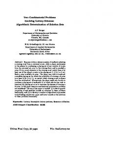
Low temperature (with H > 0)
High temperature
Figure 1.1: Examples of typical Ising con gurations at low and high temperatures.
At low temperatures the parameters J and H will have greater in uence and we are more likely to see large clusters of like spins. At higher temperatures there will tend to be less organization. Figure 1.1 shows typical con gurations for each of these cases. The Ising model can also be used to represent lattice gases, where a +1 indicates that a lattice site is occupied by a molecule and a -1 indicates it is vacant. The high and low temperature diagrams in gure 1.1 re ect the fact that at higher temperatures the gases move freely and particles do not in uence their neighbors much, while at lower temperatures particles attract each other and will tend to cluster as in the solid state. The partition function provides information about the phase transition between gaseous and solid states.
Example 2: Monomer-Dimer Systems
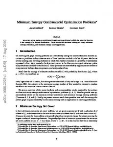
Another fundamental challenge in chemical physics is the monomer-dimer problem in which the sites of a regular lattice are covered by a non-overlapping arrangement of dimers and monomers. A dimer is a diatomic molecule which covers two adjacent vertices in the lattice, and a monomer covers each vertex not covered by a dimer (see, e.g., [30] for a 8
t t t t t t
t t t t f t
t t f t t t
f t t t t t
t t f t t t
t t t t t t
Figure 1.2: A monomer-dimer arrangement.
history of the problem). In graph theoretic terms, the monomer-dimer arrangement is just a matching; a matching of size i is a set of i lattice edges such that no two edges share a vertex. Figure 1.2 shows a typical monomer-dimer arrangement with 16 dimers and 4 monomers. The two-dimensional monomer-dimer problem serves as a model for the adsorption of diatomic molecules onto a crystal surface, where monomers correspond to empty sites [56]. The three-dimensional problem occurs classically in the theory of mixtures of molecules of di�erent sizes [20] and the cell-cluster theory of the liquid state [9]. Consider a monomer-dimer arrangement consisting of s dimers and N^ ? 2s monomers on a lattice with N^ vertices. The energy is sJ , where J is the energy derived from covering any particular edge with a dimer. Let Ms be the set of monomer-dimer arrangements with s dimers, and let jMsj be the cardinality of this set. The partition function for the canonical distribution with a xed number of dimers s is X exp(?sJ=kT ) = jMsj exp(?sJ=kT ): Zs � Zs(G; N; T ) = M 2Ms
The grand canonical distribution describes more interesting systems where the number of dimers varies. If x is the activity of a dimer, then following equation (1.2) the grand canonical distribution is
Z � Z (G; x; T ) =
^ bN= X2c
s=0
exp(?sJ=kT )xs
=
^ bN= X2c
s=0
jMsj exp(?sJ=kT )xs:
Letting � = exp(?J=kT ) � x gives gives the generating function
Z � Z (G; �) =
^ bN= X2c
s=0
jMsj �s:
(1.3)
Evaluating the coe�cients of this generating function is exactly the problem of counting the numbers of monomer-dimer arrangements with given numbers of dimers.
Example 3: Lattice Animals
A lattice animal is a set U of vertices on the lattice such that the subgraph induced by U is 9
```` ` ` ` ` ```` ` ` ` ` ```` ` ` ` ` ```` ` ` ` ` ```` ` ` ` ` ```` ` ` ` ` ```` ``` ` ` ` ` ``` ` ` ` ` ``` ` ` ` ` ``` ` ` ` ` ``t` ` ` ` ` ``t` ` ` ` ` ``` ``` ``` ``` ``` ``` ``` ``` ```` ` ` ` ` ```` ` ` ` ` ```` ` ` ` ` `t``` ` ` ` ` `t``` ` ` ` ` `t``` ` ` ` ` ```` ``` ` ` ` ` ``` ` ` ` ` ``` ` ` ` ` ``t` `0` ` ` ``` ` ` ` ` ``t` ` ` ` ` `t`` ``` ``` ``` ``` ``` ``` ``` ```` ` ` ` ` `t``` ` ` ` ` `t``` ` ` ` ` ```` ` ` ` ` `t``` ` ` ` ` `t``` ` ` ` ` t```` ``` ` ` ` ` ``` ` ` ` ` ``t` ` ` ` ` ``t` ` ` ` ` ``t` ` ` ` ` ``` ` ` ` ` ``` ``` ``` ``` ``` ``` ``` ``` ``````````````````````````````` Figure 1.3: A self-avoiding walk.
connected (see [67]). An important subclass of animals are self-avoiding walks, or animals where each vertex has degree at most two. Equivalently, a self-avoiding walk of length i starts at a xed origin and follows the lattice edges for i steps with the constraint that it never visits the same lattice site twice (see gure 1.3). The partition function here is a generating function where the coe�cients ci are the number of walks length i . Letting N^ be the number of vertices in the lattice and taking x as the monomer fugacity, the grand canonical partition function from equation (1.2) is
Z=
X
w
xjwj =
^
N X i=1
ci xi :
The self-avoiding walk models a dilute solution of long polymer chains in a good solvent. This model arises since the polymer chain can be thought of as tracing out a random walk in space, except that the physical restriction that no two molecules can occupy the same position forces the self-avoidance condition. The dilute solution enables one to study a single polymer without worrying about further restrictions caused by interactions with other polymer chains (see [48] for a survey). The more general class of lattice animals arises similarly in the study of branched polymers in dilute solution. As we have already stated, for each of these physical systems, a primary objective is to calculate the partition function. By interpreting this function as a generating function, we can instead study the underlying combinatorial problems which are intrinsically tied to these systems. The typical problem then becomes one of computing the coe�cients of the partition function; this will generally entail counting the number of con gurations in a set (e.g. the number of self-avoiding walks of length i ). We will also be interested in the problem of randomly sampling these con gurations s according to their likelihood, �(s), in the appropriate canonical distribution. Sampling allows us to examine \typical" con gurations of the system. Moreover, it has been recognized that for large classes of combinatorial problems the counting and sampling problems are closely related [36]. For 10
each of the problems we consider we will be addressing both of these questions.
1.1.2 Free energy
As indicated earlier, the partition function Z is the key to relating the microscopic and macroscopic levels of description of a physical system. While the partition function is de ned as a sum over microstates, it captures the essential information determining the macroscopic behavior of a system. In particular, the free energy F = ?kT log Z is a thermodynamic primitive from which most other thermodynamic properties can be derived. To appreciate the role of the free energy, rst consider its relation to other well-studied macroscopic functions, the entropy and the average energy of a system. The entropy, which P is de ned as S = s � (s) log � (s); represents a measure of the disorder (or \unavailable energy") of a closed system. For the canonical distribution (equation (1.1)),
kTS =
X
s
E (s) exp(?EZ(s)=kT ) ? kT log Z
= E ? F; where E is the expected (or average) energy of the system. More signi cantly, we can derive information about many thermodynamic properties of a physical system by studying how the free energy changes due to small perturbations in the xed parameters of the system. An important example is the partial derivative with respect to temperature. Discontinuities in this derivative identify phase transitions. In the ferromagnetic interpretation of the Ising model, such a phase transition corresponds to the point of spontaneous magnetization. Other examples of phase transitions are melting and boiling (see [8]). In our discussions so far we have restricted our attention to idealized nite systems where the particles coincide with lattice sites. In fact, these discrete models are really computational tools for studying the continuous analogues of the partition function and free energy on in nite lattices. The actual thermodynamic properties of a system are realized by considering successively larger lattices and studying the behavior as the lattice size tends to in nity. This is known as the thermodynamic limit. In this limit, observations regarding the behavior of the free energy determine properties of the actual system under study. In most cases there is no known way to directly compute the asymptotic behavior of thermodynamic functions, and de ning discrete analogues to these functions appears to be one of the more promising approaches. Calculating the partition function for various nite lattices therefore provides valuable insight into the corresponding real physical systems.
1.1.3 The model
Typically we think of the lattice as a nite n � n � ::: � n subgraph of the cartesian lattice Z d , although other families of lattices are also studied. In some cases it will be more appropriate to talk about nite con gurations on either an in nite lattice or a periodic lattice where opposite sides are identi ed. The choice of the lattice will be clear from the application. 11
As explained above, it is generally accepted that modeling various systems by families of successively larger lattices will tell us about the limiting continuous behavior. However, it is not immediately clear why our choice of combinatorial structures is a realistic model of the physical constraints of the particles in the systems. In particular, self-avoiding walks on the cartesian lattice appear to have a quite di�erent set of constraints from polymers, whose bond angles are rarely rectilinear. In fact the bond angles are typically tetrahedral and do not align with any regular lattice [61]. The justi cation for using self-avoiding walks to model polymers, and for the other combinatorial idealizations employed in the eld, comes from the empirical existence of universality classes. Several of the parameters studied in the thermodynamic limit appear to be dimension dependent, but lattice independent. This means that to study these universal quantities for any particular member of the class, including physically realistic models for polymers, it is su�cient to determine them for any other member. Therefore, the mathematically simpler model of self-avoiding walks on lattices lets us deduce these thermodynamic properties for the more realistic polymer models.
1.2 Computational complexity of counting problems Viewing the partition function as a generating function has identi ed several combinatorial problems as essential ingredients in understanding a physical system. Recall that when the P energy is discrete the partition function has the form i ai y i , where the coe�cient ai is the cardinality of some set of con gurations Si . For example, in the partition function of a monomer-dimer system, Si represents monomer-dimer arrangements with i dimers and ai is the number of such arrangements (see equation (1.3)). The primary combinatorial questions fall into two categories: (i) Counting: e.g., calculate ai ; the number of elements in Si . (ii) Sampling: e.g., pick an element from Si uniformly to determine the expected value of some function over the elements of Si . As explained earlier, the counting problem is used to compute the coe�cients of the partition function. The sampling problem is used to gain information about a \typical" con gura^ 2 ? 1 dimers, one might be tion. For example, in a monomer-dimer arrangement with N= interested in studying the expected distance between the two monomers. Alternatively, it is sometimes more appropriate to try to solve the weighted analogues of these problems. Here we have a set S where each element s 2 S has an associated weight w(s) = exp(?E (s)=kT ) and we are interested in the following questions: P (i) Evaluate the weighted sum s2S w(s). (ii) Generate an element of S at random according to its weight. Solving the weighted counting problem would allow us to calculate the partition function directly, although we would not know all of the individual coe�cients. Both the unweighted and weighted versions of the counting and generation problems will fall into a similar framework. 12
Ideally we would like analytic solutions to the counting (or weighted counting) problems. In 1944, Onsager discovered such a closed-form expression for the partition function of the two-dimensional Ising model with zero external eld [53]. It has not been possible to nd such a precise solution for most other physical systems, or even for the Ising model in higher dimensions or in the presence of an external eld. Consequently most of the research in recent years has been concentrated on designing e�cient algorithms to solve the counting and generation problems. Algorithms based on Monte Carlo simulations, in particular, have provided great insight into various physical systems. However, while they are useful tools, many of the algorithms actually used in statistical mechanics are nonrigorous applications of the methods and are not reliable. Recent progress in the design of provably accurate and e�cient approximation algorithms enables us to develop new Monte Carlo algorithms with guaranteed error bounds.
1.2.1 E�cient algorithms For an algorithm to be practical, it must be e�cient in the sense that its running time does not grow too fast with the input size. The generally accepted formalization of the notion of e�ciency is a polynomial-time algorithm. Such an algorithm takes as input a natural description of the problem instance and must compute an output in time which is bounded by some xed polynomial in the size of the input description (see, e.g., [31]). For problems in statistical mechanics involving lattices, the input size is taken to be N^ , the number of vertices in the lattice; a polynomial-time algorithm (e.g., for the counting or generation problems) must solve the problem in O(N^ k ) time, for some xed k . This is a natural measure of the input size since the number of solutions is exponential in N^ and it requires O(N^ ) steps just to write down a typical con guration. Note that, for any of the physical problems presented in section 1.1, it is trivial to design an exponential-time algorithm which computes the output in time exp(O(N^ )). Since the number of con gurations on a lattice of size N^ is at most exponential in N^ , we can do this by exhaustively enumerating each con guration. Of course such an algorithm is not polynomial-time and is impractical unless the size of the lattice is very small. We should also note that polynomial-time algorithms are not necessarily e�cient in practice; for polynomials with large degree it might be infeasible to run the algorithm except for small inputs. However, a polynomial-time algorithm is certainly a dramatic improvement over a trivial exponential-time one, and typically such algorithms are later improved so as to be genuinely practical. A breakthrough in the design of e�cient algorithms in statistical mechanics was achieved in 1961 when Fisher, Kasteleyn and Temperley independently discovered a polynomial-time algorithm for a special case of the monomer-dimer problem known as the dimer problem [15,40, 63] (see section 2.1). The dimer problem asks for the number of perfect matchings, ^ 2 dimers (and no monomers). (More generally, a perfect or coverings of the lattice by N= matching in a graph is a matching in which every vertex of the graph is incident to some edge in the matching.) The Fisher, Kasteleyn, Temperley technique generalizes to counting perfect matchings in any planar graph and can also be used to construct a polynomial-time algorithm for the partition function of the two-dimensional Ising model with zero external eld. 13
Despite major e�orts to generalize these techniques, it does not appear that they can be used to solve the monomer-dimer problem in the presence of monomers or the Ising model in non-zero eld, even in two dimensions. Similarly, the techniques rely critically on planarity and do not appear to generalize to higher dimensional lattices. The rst formalization of this limitation came when Hammersley et al. [25] proved that there cannot be a straightforward way of extending the above approach to even three-dimensional lattices.
1.2.2 Hardness Computational complexity theory o�ers further evidence for the apparent hardness of these problems. In 1979, Valiant de ned the class #P to classify counting problems [64]. A counting problem asking for the number of elements in a set Sn representing con gurations on a graph G belongs to #P if there is a non-deterministic polynomial-time Turing machine with input n and G such that the number of accepting computations is exactly jSnj; the number of elements in Sn . Note that this is exactly the framework for the class NP; while NP is the set of problems for which the non-deterministic machine decides whether an accepting computation exists, #P is the class of problems for which the non-deterministic machine counts how many accepting con gurations exist (see [18] for a survey). Each of the computational problems from the previous section can be expressed as a general graph theoretic problem. For instance, the problem #MATCHING( G; i ) takes as input a graph G and an integer i and asks how many matchings of size i exist. This problem is in #P since we can construct a non-deterministic Turing machine which \guesses" a set of edges of G and then checks, in time polynomial in N^ (the number of vertices of G ) whether this is actually a valid con guration. Similarly, #SAW( G; i; x0 ) takes as input a graph G , and integer i and a designated vertex x0 and asks for the number ci of self-avoiding walks of length i starting at the vertex x0 . Finally, #ISING( G; E ) takes as input a graph G and asks how many con gurations have a particular energy E . These problems are also in #P since we can design a non-deterministic algorithm which guesses a candidate con guration and then decides, in polynomial time, whether this con guration should be included in the count. The class #P has a subclass of complete problems which characterize, in a precise sense, the hardest problems in the class. To formalize this we need the following de nition. For any two counting problems A and B , A is polynomial-time Turing reducible to B if there exists a polynomial-time algorithm for A which uses B as a subroutine. Thus, if A is polynomialtime reducible to B , then the existence of a polynomial-time algorithm for B implies that one also exists for A . A problem B is # P-complete if every problem in #P is polynomialtime reducible to B . Thus, showing that any #P-complete problem can be solved in polynomial time would imply that there is a polynomial time algorithm for every problem in #P . #P-completeness is regarded as strong evidence of intractability: exhibiting a polynomial time algorithm for any #P-complete problem would provide e�cient solutions to many hard problems such as counting the number of satisfying assignments of a boolean formula. Since it is expected that no polynomial-time algorithm can even decide whether a satisfying assignment exists, it is even more unlikely that an e�cient algorithm exists to count the number of satisfying assignments. ^ 2), the problem of counting perfect matchValiant showed that #MATCHING(G; N= 14
ings in a graph with N^ vertices, is #P-complete [64]. This helps explain why Fisher, Kasteleyn and Temperley's algorithm fails to generalize to all non-planar graphs. Furthermore, Jerrum showed that counting the total number of matchings (of all sizes) in a graph is #P-complete, even when the graph is planar [32]. This gives evidence for why the Fisher, Kasteleyn, Temperley algorithm does not easily generalize to counting matchings of arbitrary size. Similarly, consider the problem #SAW( G; N^ ? 1; x0 ) which asks us to count self-avoiding walks of length N^ ? 1 on a graph G with N^ vertices starting from x0 . This is just the problem of counting the number of Hamiltonian paths starting at x0 , another problem known to be #P-complete. Of course we cannot claim that these #P-complete problems, which are hard when given an arbitrary graph as input, remain hard when the input graph is restricted to be a lattice. Nonetheless, these hardness results do suggest that any polynomial-time algorithm to solve these problems must use properties of the lattice in a non-trivial manner. No polynomial-time algorithm which does this is known. In fact, exploiting lattice properties to design e�cient algorithms has proven to be notoriously di�cult. While initially discouraging, the #P-completeness of many important combinatorial problems has shifted focus towards designing e�cient approximation algorithms. An approximation algorithm uses randomization to produce a close estimate to the true answer with high probability. Recently there has been much progress in the design and analysis of e�cient randomized algorithms for approximately counting. Approximation algorithms are generally su�cient for combinatorial problems arising from statistical mechanics since we are interested in studying the limiting behavior of quantities associated with the system, and these algorithms allow us to approximate the true values to arbitrary precision.
1.3 Approximation algorithms Approximation algorithms based on computer simulations of a random process have assumed an important role for a wide range of combinatorial problems. The idea is as follows. Let S be a large but nite set of combinatorial structures. Much information about S can be gained by sampling elements of S according to an appropriate probability distribution � . For example, suppose that � is chosen to be the uniform distribution. At least intuitively, sampling elements uniformly is useful for studying properties of a typical element of S . In fact, sampling uniformly turns out to be a useful tool for approximate counting as well. More formally, we will be interested in designing algorithms which meet the following speci cations. These are the standard de nitions of approximation algorithms for counting and sampling (see, for example, [39, 36, 59]). Let Sn be the set of con gurations of size n on a lattice G of size N^ (for example, Sn might be the set of self avoiding walks of length n on an N^ 1=2 � N^ 1=2 lattice). Let an be the number of elements in Sn . De nition 1.3.1 A randomized approximation scheme for an on a lattice G of size N^ is a probabilistic algorithm which, on input n , G and � , � 2 (0; 1) , outputs a number f (G; n) such that Prfan (1 + �)?1 � f (G; n) � an (1 + �)g � 1 ? � . The approximation scheme ^ �?1 is fully-polynomial, or an fpras, if it is guaranteed to run in time polynomial in N; ? 1 and log � . 15
De nition 1.3.2 An almost uniform generator for Sn on a lattice G of size N^ is a probabilistic algorithm which, on input n , G and � 2 (0; 1) , outputs an element � of Sn with probability at least 1=q (N^ ) for a xed polynomial q , such that the conditional probability distribution over elements of Sn has variation distance� at most � from the uniform distribution. The generator is fully-polynomial, or an fpaug, if it runs in time polynomial in N^ and log �?1 .
The parameter � determines the accuracy required of the estimate, while � controls the con dence level. A fully-polynomial randomized approximation scheme provides an e�cient means of numerically computing f , in the sense that its running time grows only slowly (i.e., polynomially) with the lattice size N^ , the accuracy parameter � , and the con dence parameter � . Similarly, a fully-polynomial almost uniform generator gives an e�cient means for solving the sampling problem. In the cases we are interested in, Sn represents some exponentially large set of combinatorial objects such as self-avoiding walks of length n , so naive methods based on exhaustive enumeration are infeasible. Instead we will focus on designing an e�cient solution to the corresponding sampling problem and then show how this will provide a tool for solving the counting problem. Suppose we want to sample from Sn according to some distribution � . The standard approach is to simulate a Markov chain whose state space ? includes Sn . At each point in time t we visit a combinatorial structure s 2 ?. In the next time step, we move to a (possibly) new structure by performing some random local perturbation to the structure s . For example, let Sn is the set of self-avoiding walks of length n and suppose we want to sample a walk in Sn uniformly. We can let ? be the set of self-avoiding walks of length at most n , and choose a distribution � 0 on ? such that the conditional probability of � 0 on Sn is the uniform distribution. To simulate the Markov chain we start at the empty walk w0 . At any point in time, if we are currently at a self-avoiding walk w , then at the next step we move, with some appropriately chosen probability, to a walk w0 2 ? which di�ers from w by at most one edge. After iterating this process for a su�cient number of steps t^, we examine the walk w^t . If w^t 2 Sn , then we output it; otherwise we start again. In order for this method to satisfy the requirements of a fully-polynomial almost uniform generator (see de nition 1.3.1), the nal distribution from which we are sampling must be reasonably well concentrated on Sn (so that one gets a valid sample quite often), and the Markov chain must converge rapidly to its stationary distribution (so that the number of simulation steps required is not too large). Guaranteeing all of these conditions for a particular Markov chain can be di�cult. Already Monte Carlo algorithms based on Markov chains appearing to satisfy these properties are used extensively in the physical sciences. These simulations have provided great insight into the asymptotic behavior of physical systems, but they are often nonrigorous. The most common di�culty arises from not knowing how long to simulate the Markov chain. A sample taken after simulating the Markov chain for too few steps might be chosen according to an unknown distribution which is quite far from the stationary distribution. Consequently, � The variation distance measures the distance between two distributions �1 , �2 over Sn and is de ned P as k�1 ? �2 k = 12 s2S j�1 (s) ? �2 (s)j = maxA�S j�1 (A) ? �2 (A)j .
16
statistics inferred from such samples might appear to have similar properties to those being tested and yet the results would in fact say nothing about the true distribution being studied. Therefore it is necessary to rigorously show that the Markov chain has the desired properties and is simulated a su�cient number of steps.
1.3.1 Markov chains
All of the Markov chains we will be using are variants of the Metropolis algorithm discovered in 1953 [49]. We will review some of the concepts of Markov chains in the context of this algorithm. Again, assume we have a set S from which we want to sample according to a distribution � . We de ne the Markov chain on a possibly larger state space ? containing S . First we choose a graph H underlying the Markov chain whose vertices are the states in ?. Every element i 2 ? has a small number d � d^ of neighbors in H . Furthermore, assume that for any edge (i; j ) in H , we have an \acceptance probability" A(i; j ) 2 (0; 1]. The Markov chain is designed so that if we take a random walk along the edges of H according to the transition probabilities starting at any state, then we will eventually converge to a stationary (or equilibrium) distribution � 0 over the state space ?. We choose the graph H and the transition probabilities A so that the stationary probability of being in S � ? is not too small, and so that the conditional probability � 0 (s)=� 0(S ) of being at any particular state s 2 S is � (s). If we know the stationary distribution in advance, then by simulating the Markov chain for su�ciently many steps, we can sample according to this distribution. We always choose the graph H so that it is connected; i.e., it is possible to get from any state of the Markov chain to any other state; such a Markov chain is called irreducible. If, in addition, we know that there is a time t when it has positive probability of being at each state, then the chain is aperiodic. A Markov chain with both of these properties is ergodic and there is a unique stationary distribution � 0 to which the Markov chain converges. The transition probabilities are de ned as follows. Starting at an arbitrary point i 2 S we perform the following steps: (i) Choose a random neighbor j of i , each with probability 1=d^. (ii) Move to j with probability A(i; j ); otherwise stay at i . Then the transition probabilities are represented by a matrix P where P (i; j ) = A(i; j )=d^; if i 6= j , and
P (i; i) = 1 ?
X
j 6=i
A(i; j )=d^:
In the Metropolis algorithm we de ne A(i; j ) = min(1; � 0(j )=� 0(i)): It is then easy to verify that P (i; j ) satis es the detailed balance equation �0(i)P (i; j ) = � 0 (j )P (j; i): (1.4) Informally, the detailed balance equation says that at stationarity the Markov chain is equally likely to move from i to j as the other way around. A Markov chain which satis es 17
this condition for all states i and j is called reversible, and � 0 is the unique stationary distribution to which the Markov chain converges, starting at any initial state. All the Markov chains we will be using are reversible. This framework lets us design Markov chains which will eventually converge to a particular conditional distribution � on our state space S . For this to be useful for e�ciently sampling according to � , we need to bound the rate of convergence. This property is called the mixing rate of the Markov chain. Since the state space is typically exponentially large (in the description of the combinatorial problems we are using it for), we need a strong condition which says that after only a polynomial number of steps we are close to stationarity. This is called rapid mixing and can be characterized by the expansion properties or conductance of the graph underlying the Markov chain [59, 34]. We will explain this connection in greater detail in section 3.2.2.
1.4 Summary The remainder of this thesis is divided into two chapters. The rst chapter addresses the monomer-dimer problem. We show that there is a fully-polynomial randomized approximation scheme for counting the number of matchings of any cardinality on any periodic nite lattice (or, more generally, any Cayley graph.) A periodic lattice includes \wrap-around" edges which make the lattice into a torus. These results also extend to counting matchings on non-periodic planar lattices. This gives an approximation algorithm which solves the monomer-dimer problem in exactly the two cases where the Fisher, Kasteleyn, Temperley algorithm fails: namely, counting matchings of arbitrary size, and counting matchings on non-planar lattices. These results are based on an approximation algorithm due to Jerrum and Sinclair [34] and Broder [7]. In each of these cases we also present an almost uniform generator for the corresponding sampling problems. This chapter is based on work with Claire Kenyon and Alistair Sinclair [43]. In chapter 3 we address the problem of counting self-avoiding walks in lattices. We present a \testable algorithm" to solve this problem. We introduce the notion of a testable algorithm to describe an e�cient algorithm whose correctness is based on a conjecture which the algorithm systematically veri es. The algorithm either discovers a counterexample to the conjecture or produces numerical answers which are correct with high probability. Therefore, any outputs produced by the algorithm are correct. We design such an algorithm for counting and generating self-avoiding walks in any nite rectangular lattice in arbitrary dimension. The algorithm relies on a single conjecture which is widely accepted in the physics community. Consequently, we expect that the algorithm will always output correct numerical outputs; on the other hand, should the algorithm nd that the conjecture is incorrect, this would have interesting implications as well. These are the rst algorithms for counting and generating self-avoiding walks where the error bounds are rigorously controlled. These results are based on work with Alistair Sinclair [54]. An optimized version of the algorithm was implemented by Rob Pike yielding numerical estimates for the number of self-avoiding walks in 2 and 3 dimensions; these estimates are presented in section 3.5.
18
Chapter 2
Matchings 2.1 Introduction
2.1.1 Historical background
The rst problem we consider is the monomer-dimer problem, in which the sites of a regular lattice are covered by a non-overlapping arrangement of monomers (molecules occupying one site) and dimers (molecules occupying two sites that are neighbors in the lattice). For a given monomer-dimer arrangement with d dimers and N^ ? 2d monomers on a lattice of size N^ , the dimer density is de ned as 2d=N^ . We are interested in counting the number of monomer-dimer arrangements with any xed density. In this section we present some of the highlights in the history of this problem. For further information see, e.g., [30, 42, 66] and the references given there. The monomer-dimer problem gained prominence in 1937 through the early paper of Fowler and Rushbrooke [17]. A breakthrough was achieved in 1961, when, independently, Fisher, Kasteleyn and Temperley provided an analytic solution for the case of dimer coverings (i.e., arrangements with dimer density 1) on a two-dimensional rectangular lattice [15, 40, 63]. The key idea is to express the number of dimer coverings as a Pfa�an, which in turn can be evaluated as the square root of an associated determinant. These calculations give precise asymptotics for f (n), the number of dimer coverings of an n � n rectangular lattice (with n even); speci cally, 1 ln f (n) ! � as n ! 1 , where � = 1 X (?1)r = 0:29156::: n2 � r�0 (2r + 1)2 Moreover, since the problem is reduced to evaluation of a determinant, the quantity f (n) can be computed numerically for any value of n in an e�cient manner. In fact, this technique is more general and allows the number of dimer coverings of any planar graph (or indeed of any family of graphs with xed genus) to be computed e�ciently [41]. Unfortunately, these methods do not extend to two-dimensional lattices with dimer density less than 1, or to lattices in higher dimensions even when the dimer density remains 1. In fact, the three-dimensional dimer covering problem, which asks for the number, f (n), of ways of lling an n � n � n rectangular lattice with dimers, is one of the classical unsolved problems of solid-state chemistry. A few facts are known: for example, ln(f (n))=n3 tends 19
to a nite limit � as n tends to in nity [21]. Hammersley [22] proved the lower bound � � 0:418347, while the early paper by Fowler and Rushbrooke [17] showed the upper bound � � 0:54931. It has been conjectured that � lies between 0:43 and 0:45. In other work, Bhattacharjee et al [4] studied the phase transition behavior of the three-dimensional model. However, no reliable method is known for computing f (n) to good accuracy. A similar lack of rigorous results holds for the problem at dimer densities less than 1, even in two dimensions. Notable exceptions are series expansions valid at low densities [19] and lower bounds on the free energy [6, 26].
2.1.2 Results We make progress on the monomer-dimer problem in cases where the technique of Fisher, Kasteleyn and Temperley fails. Speci cally, we give a polynomial-time algorithm for computing, to arbitrary precision, the number of coverings of a rectangular lattice in any dimension with any speci ed dimer density. More precisely, for a xed dimension d , let G be the d -dimensional rectangular lattice [1; : : :; n]d (with periodic boundary conditions). We let f (G; s) denote the number of coverings of G by s dimers and nd ? 2s monomers. Our main result is a fully-polynomial randomized approximation scheme (see de nition 1.3.1) for computing the function f (G; s) above for rectangular lattices of any dimension d . This extends previous computational techniques in two ways. First, it enables one to compute the number of dimer coverings in lattices in three and higher dimensions. And second, it enables one to count coverings with dimer density less than 1, a problem that was not approachable by the methods of Fisher, Kasteleyn and Temperley even in two dimensions. Our algorithm provides a feasible approach to numerical computation of quantities such as f (n), the number of dimer coverings of an n � n � n rectangular lattice in three dimensions. This is apparently the rst such method whose running time provably grows only polynomially with n . We should, however, inject three caveats here. First, the running time of the algorithm, though polynomial, is not small enough to be genuinely practical; nonetheless, it is quite likely that careful honing of the algorithm and its analysis will lead to a practical method. Secondly, the algorithm provides only statistical estimates of f , rather than precise values; we stress, however, that the error bars on these estimates can be made arbitrarily small, and, in contrast to previous Monte Carlo approximation methods, are completely rigorous and require no assumptions of any kind. Thirdly, although the algorithm allows f (n) to be computed e�ciently for each n , we do not provide bounds on the time required to compute the asymptotics of f (n) as n tends to in nity, and therefore the entropy � . This would require, in addition, bounds on the rate of convergence of the series ln(f (n))=n3 . The above result holds for lattices with periodic boundary conditions (i.e., the edges of the lattice are \wrapped around" to make it toroidal). In the two-dimensional case, our method extends to lattices with xed boundaries: i.e., we again get a fpras for computing the number of coverings with any speci ed dimer density. This result again goes beyond the technique of Fisher, Kasteleyn and Temperley for planar graphs, which holds only for 20
dimer density 1.� Finally, we can extend the above results to a broader class of lattices. Speci cally, we get a fpras for counting coverings, with any speci ed dimer density, of any bipartite graph that is the Cayley graph of some nite group. This includes other commonly studied lattices such as the hexagonal lattice with periodic boundary conditions.y
2.1.3 Overview of the algorithm
The algorithms mentioned above are all based on a Monte Carlo procedure due to Jerrum and Sinclair [34] and Broder [7], for approximating the number of matchings in a graph. A matching in a 2m -vertex graph G = (V; E ) is any subset M of the edge set E such that no two edges in M have a common endpoint. Clearly, matchings of cardinality s correspond precisely to monomer-dimer arrangements in G with s dimers and 2(m ? s) monomers. The classical monomer-dimer problem discussed in the previous two subsections is the special case in which G is the d -dimensional rectangular lattice [1; : : :; n]d for some d . Let us now associate with each matching M in G a weight w(M ) = �jM j , where jM j denotes the cardinality of matching M and � is a positive real number. Recall that the monomer-dimer partition function (or generating function ) of G is
Z (G; �) =
X
M
w(M ) =
m X s=0
a s �s ;
where the coe�cient as is the number of matchings in G of cardinality s (see equation (1.3)). Thus, in the monomer-dimer problem on G , we are trying to compute the coe�cients as for various values of s . The Monte Carlo method described in [34] simulates a Metropolis-style Markov chain whose state space is the set of matchings in G (see section 1.3.1). The stationary distribution of the Markov chain is jM j �(M ) = Z �(G; �) :
The stationary probability of a matching M is proportional to its weight, and the normalizing factor is just the partition function. Transitions correspond to local random perturbations such as the addition, deletion or exchange of an edge of the matching. More precisely, suppose we are at a state M (a matching in G ). The graph H underlying the Markov chain is de ned so that each state M � If the number of monomers is some xed constant 2c (so that the dimer density tends to 1 as n
! 1) then the Fisher, Kasteleyn and Temperley technique can in principle be used, as follows. For each possible set of 2c positions for the monomers, use the technique to count dimer coverings in the graph formed by removing these sites from the lattice: this works because the graph remains planar. Now sum over all possible positions for the monomers. However, this approach no longer runs in polynomial time if c is allowed to grow with n , and is ine�cient even for quite small xed values of c . y An analytic solution to the dimer covering problem for this planar lattice has been known for some time
[65, 41]. In contrast to the rectangular lattice, the assumption of periodic boundary conditions is important here: Elser [14] has solved the dimer covering problem on a hexagonal lattice with xed boundaries, and shown that the result depends signi cantly on the shape of the boundary.
21
has at most jE j neighbors, where jE j is the number of edges in G . To move to a new state, we rst randomly choose an edge from the graph G . Either the edge e corresponds to a new state M 0 (in a manner to be described), in which case we move to M 0 with probability A(M; M 0); otherwise we remain at M . When � < 1 the transitions of the Markov chain are as follows.z (i) if e 2 M , move to the state M 0 = M ? e (i.e., A(M; M 0) = 1). (ii) if exactly one of the vertices u or v is matched by an edge e0 2 M , move to the state M 0 = M ? e0 + e (i.e., A(M; M 0) = 1). (iii) if neither endpoint of e is matched in M , move to the state M 0 = M + e with probability A(M; M 0) = � . (iv) in all other cases do nothing. This Markov chain is ergodic and reversible, and from the detailed balance equation (1.4) it is easy to see that the unique stationary distribution is � . The case de ned above for � < 1 is of greater physical interest, but for computation purposes it is also useful to de ne the Markov chain for � � 1. The Markov chain has the same underlying graph H , so a matching M has the same set of neighbors as the Markov chain de ned above. The new transition probabilities are de ned as A(M; M 0) = 1=� if M 0 is formed by removing an edge from M , and A(M; M 0 ) = 1 if M 0 is formed by adding or exchanging an edge. Again from the detailed balance equation it follows that the stationary distribution is � . The algorithm works by observing this process at equilibrium for various values of � . By running a series of experiments, using suitable values of � , we can estimate the successive ratios of coe�cients ai =ai?1 . If our estimates are su�ciently good, then appropriate products of these estimates would yield an estimate for each of the coe�cients ai . For the details of the algorithm, see [34]. The dominant factor in the running time of this algorithm is the number of steps that need to be simulated in order for the Markov chain to reach equilibrium for the values of � needed in the above experiments. This quantity is analyzed rigorously in [34] and shown to be a polynomial function of the ratio �(G) = am?1 =am , speci cally O(�(G)4jE j2). (This has since been improved to O(�(G)2jV jjE j); see [58].) The Monte Carlo procedure will therefore be e�cient for graphs G in which the ratio �(G) is small.x Matchings in G of cardinality m are called perfect matchings, and those of cardinality m ? 1 are called near-perfect matchings : these correspond respectively to dimer coverings and coverings with precisely two monomers. The ratio �(G) measures the amount by which the number of near-perfect matchings in G exceeds the number of perfect matchings. z The transition probabilities of the actual Markov chain described in [34] are a slight variant of these
where we allow self-loops at each state to ensure aperiodicity.
x In [34, 59] it is shown that the same approach yields a fpras for the partition function Z | though
not for all its coe�cients | in an arbitrary graph, regardless of the value of �(G). Moreover, it is also possible to obtain all the coe�cients as with s � (1 ? � )m , in time polynomial in m1=(1?�) . This enables one to approximately count the number of coverings with xed dimer density p = 1 ? � , for � > 0, but the running time grows exponentially with p?1 .
22
Note that this ratio is always at least m , since the removal of any edge from a perfect matching yields a unique near-perfect matching. For an e�cient algorithm, we want the ratio to be not too much larger than m : speci cally, for a fpras it must be bounded above by a polynomial function of m for the family of graphs in question. Note that this is not a trivial property: it is not hard to construct a family of 2m -vertex graphs, m = 1; 2; : : :, for which the ratio grows exponentially with m . We will discuss this issue in more detail in section 2.4. Our main technical contribution is to prove that the ratio is small for lattices and, more generally, for arbitrary Cayley graphs. Speci cally, we show that if G is the d -dimensional rectangular lattice [1; : : :; n]d with periodic boundary conditions (so that m = 21 nd ), then �(G) � m2 = 41 n2d . This ensures that the Monte Carlo algorithm is in fact a fpras: i.e., its running time grows only polynomially with n for any xed dimension d . A similar bound holds for arbitrary Cayley graphs. We stress that our Monte Carlo algorithm di�ers from earlier ones for monomer-dimer systems (see, e.g., [23]) in that it is guaranteed (independent of any heuristic arguments) to provide statistically reliable estimates in a running time that grows only polynomially with the number of lattice sites. Our proofs of the above bound for lattices and Cayley graphs, presented in the next two sections, are elementary and rely on a novel \translation" technique: the strong symmetry properties of the lattice (and of arbitrary Cayley graphs) allow any matching (monomerdimer con guration) to be translated, which in turn permits the symmetry to be broken. We conjecture that this technique may shed more light on other quantities related to monomerdimer systems, and in particular the correlation between monomers at two speci ed sites, as studied in two dimensions by Fisher and Stephenson [16]. The remainder of the chapter is organized as follows. In the next section, we prove bounds of the above form for rectangular lattices with periodic boundary conditions in any dimension, and with xed boundaries in two dimensions. In section 2.3 we extend our technique to handle arbitrary Cayley graphs. Finally, in section 2.4 we conclude with some further remarks on the physical and combinatorial signi cance of the above ratio, together with some open problems.
2.2 Rectangular Lattices We begin by introducing some de nitions and notation concerning lattices. We will be interested in two classes of lattices: the rst class are those with xed boundary conditions, in which the lattice is not perfectly regular but has distinguished boundary vertices. Thus, we consider the d -dimensional rectangular (or cartesian) lattice L(n; d), where the vertices are the nd integer lattice points in [1; n]d , and two points x; y are connected by an edge i� they are unit distance apart. The second class is lattices with periodic boundary conditions, in which the lattice includes wrap-around edges to make it toroidal; that is, we augment L(n; d) with an edge between (x1; : : :; xi?1 ; n; xi+1; : : :; xd ) and (x1 ; : : :; xi?1 ; 1; xi+1; : : :; xd), for each i . We will write Le (n; d) for the periodic lattice. We shall adopt the terminology of graphs and matchings introduced in section 2.1.3. We view L(n; d) and Le (n; d) as graphs with 2m = nd vertices, and we always assume that n is even, so that both L(n; d) and Le (n; d) contain a perfect matching (dimer covering). For any 2m -vertex graph, we let M be the set of perfect matchings and N the set of 23
near-perfect matchings (monomer-dimer coverings with exactly two monomers). In any matching (monomer-dimer covering), we refer to the set of unmatched vertices in the graph as holes, and we write N (u; v ) for the set of near-perfect matchings with holes u and v . All the graphs we consider will be bipartite, with m vertices on each side of the bipartition. It will sometimes be convenient to view the vertices on one side of the bipartition as being colored white, and those on the other side black. (In the case of the two-dimensional lattice, this coloring corresponds to the usual black and white coloring of the checker-board squares which form the dual graph.) Note that in any near-perfect matching, one hole is white and the other black. Recall from the previous section that our aim is to construct e�cient approximation algorithms for the number of monomer-dimer coverings of various lattice graphs with any speci ed number of dimers. As indicated earlier, all our algorithms are based on an earlier result of Jerrum and Sinclair about counting matchings in a graph subject to a certain condition on the graph. We now state this result precisely. Recall that, for a 2m -vertex graph G , the quantity �(G) = jNj=jMj is de ned to be the ratio of the number of nearperfect matchings to the number of perfect matchings in G .
Theorem 2.2.1 (Jerrum and Sinclair [34, Theorem 5.3]) There exists a fpras for the number of perfect matchings in any family of 2m -vertex graphs G that satis es �(G) � q (m) , for a xed polynomial q . The remark following this result in [34] points out that this polynomial relationship between the numbers of near-perfect and perfect matchings also allows one to construct a fpras for counting matchings of arbitrary cardinality in G . We now proceed to prove that such a relationship does in fact hold for families of lattice graphs, and (in the next section) for more general Cayley graphs. The technique that we use in our proofs relies on the structure of the union of two matchings in a graph. Consider the subgraph C consisting of the union of the edges in two perfect matchings M1 and M2 . If we color the edges from M1 red and those from M2 blue, we nd that every vertex is adjacent to exactly one red edge and one blue edge, so C is the union of even-length cycles, each of which alternates colors. (Some of these cycles may be trivial, consisting of a single edge colored both red and blue.) Clearly the converse is also true, i.e., any covering of the graph with even-length cycles which alternate colors de nes two perfect matchings: the set of red edges and the set of blue edges. Similarly, suppose we have two near-perfect matchings, N1 with holes u and v , and N2 with holes u0 and v 0 , where u; u0; v and v 0 are distinct vertices. Then in the subgraph C de ned by the union of the red edges N1 and the blue edges N2 , vertices u; u0; v and v 0 all have degree one and all other vertices have degree two. So C consists of even-length alternating cycles, plus two alternating paths whose endpoints are u; u0; v and v 0 . Moreover, either both of these paths have even length or both have odd length. See gure 2.1. Our proofs rely on the observation that, if u0 is a neighbor of u and v 0 is a neighbor of v , then by augmenting C with edges (u; u0) and (v; v 0), we can ensure that every vertex has degree two. When the graph is bipartite, the resulting subgraph must consist solely of even-length cycles, and therefore the cycle containing u and u0 must also contain v and v 0 . By recoloring some of the edges on this new cycle, we can force it to alternate colors so that 24
r r r r r r
r r r r r r
r r r r r rdu
r r r r r r
r r r r rdv r
r r r r r r
-
qqqqqq r r rqqqqqqr rqqqqqqr qqqqqq r r rqqqqqqr rdv0 qr dru0 rqqqqqqr rqqqqqqr qqr rq rq rqqqqqqr rqqqqqqr rqq rqq rqq rqqqqqqrdv qqr r r rqdu rqqqqqqr qr qqqqqq
�
qqqqqq r r qqqqqq r r rqqqqqqr qqqqqq r r qqqqqq r r rdv0 rq dru0 qqqqqq r r rqqqqqqr rqq qr qr rqqqqqqr rqqqqqqr qqr rqq rq rqqqqqqr rq q q qqqqqq r r rq rqqqqqqr rq
Figure 2.1: The union of two near-perfect matchings.
the cycle cover de nes two perfect matchings. We use this observation to de ne a mapping from the set of pairs N (u; v ) � N (u0; v 0) to the set of pairs M � M that is injective, which in turn, by virtue of the symmetry properties of the lattice, implies that jNj is not much larger than jMj . We are now in a position to state our rst result. Theorem 2.2.2 For the d -dimensional periodic lattice Le(n; d) , the ratio �(Le (n; d)) is bounded above by n2d =4 . Before proving this theorem, we combine it with Theorem 2.2.1 to obtain the following immediate corollary. Corollary 2.2.3 There exists a fpras for the number of monomer-dimer coverings with any speci ed number of dimers in the d -dimensional periodic lattice Le (n; d) , for any xed dimension d .
Proof of Theorem 2.2.2. Let M and N be the sets of perfect and near-perfect matchings respectively in Le (n; d), so that �(Le (n; d)) = jNj=jMj . First we x two holes, u and v .
Let u0 be the neighbor one to the right of u , i.e., u0 = u + (1; 0; :::; 0) mod n . Similarly, let v 0 be the neighbor one to the right of v . We proceed to construct an injection � from N (u; v ) � N (u0; v 0) into M � M . To do this, let N1 2 N (u; v ) and N2 2 N (u0; v 0), and consider the subgraph C of Le (n; d) de ned by the union of red edges N1 , blue edges N2 and special edges (u; u0) and (v; v 0). If we color the special edges red, then u0 and v 0 are each adjacent to two red edges, and every other vertex is adjacent to one edge of each color; if we now ip the colors of the edges along one of the paths from u0 to v 0 , every vertex will be adjacent to exactly one edge of each color. To avoid ambiguity, we choose the path from u0 to v 0 which does not pass through u . As we saw earlier, the sets of colored edges now de ne two perfect matchings. See gure 2.2. We need to check that this map � is injective: given any pair of perfect matchings (M1; M2 ) in the image of the map, we show that we can uniquely reconstruct the pair of near-perfect matchings, one with holes u and v and the other with holes u0 and v 0 , that are mapped by � to (M1; M2). Note that the union of any pair of matchings in the image of � always contains an alternating cycle that includes the edges (u; u0) and (v; v 0). Now 25
rqqq rqqq rqqq rqq q q q qr rqqq rqqq rqqq rqqq rqq q q q qr rqqq drqqqu dru0 rqq q q q qr rqq q q q qr rqqq rq qq q q qr rqq q q q qr qqqr rq qq q q qr rqq q q q qdrv dr v0 qqqr qr qq q q qr qqr q q q qr qqr q q q qr
-�
qqqr qqqr qqqr qqqr dqqqru dqqqru0 qqqr qqqr rq q q q q rq qr q q q q qr
qqqr qr q q q q qr qqqr qqqr qr q q q q qr qqqr qr q q q q qr qr q q q q qr qr q q q q qr qqqr qqqr rq q q q q dqrv qdqqr v0 qqqr qr q q q q qr qr q q q q qr
Figure 2.2: Mapping two near-perfect matchings to two perfect matchings.
color the edges of the matching containing (u; u0) red, and the edges of the other matching blue. By ipping the colors of the edges along the path from u0 to v 0 (again choosing the path which avoids u , for consistency), we make u0 adjacent to two red edges. Since u0 and v0 are the holes of some near-perfect matching, they lie on opposite sides of the bipartition and any path between them must have odd length. Therefore, after the ipping operation v0 must be adjacent to two red edges as well, while all other vertices are still adjacent to one edge of each color. If we now remove the edges (u; u0) and (v; v 0), the colored edges must correspond to the two near-perfect matchings that are mapped by � to (M1; M2). The above construction demonstrates that jN (u; v )j � jN (u0; v 0)j � jMj2 . To nish the proof, we use the structure of the lattice Le (n; d): in a periodic lattice, the operation of shifting a matching one position to the right is a bijection between the sets N (u; v ) and N (u0; v0), so jN (u; v)j = jN (u0; v0)j . Thus the above relationship gives jN (u; v)j2 � jMj2 , which implies jN (u; v )j � jMj . Summing over all choices of a black vertex u and a white vertex v , we nd that jNj � n2d jMj=4, so that �(Le (n; d)) � n2d =4, as claimed.
Remark. It should be clear from the above proof that Theorem 2.2.2 (and hence Corol-
lary 2.2.3) generalizes to \hybrid" lattices that have xed boundary conditions in some dimensions provided there exists at least one dimension in which the lattice has periodic boundary conditions. It also holds in more general bipartite rectangular lattices of size n1 � n2 � ::: � nd with periodic boundary conditions (i.e., for any dimension i in which the boundary is periodic, ni must be even). The following theorem extends the above technique to handle two-dimensional lattices with xed boundaries. We again show that in these lattices the number of near-perfect matchings cannot be too large compared to the number of perfect matchings, and then appeal to Theorem 2.2.1. Theorem 2.2.4 For the two-dimensional lattice with xed boundaries L(n; 2) , the ratio �(Le (n; d)) is bounded above by n4 =4 . Corollary 2.2.5 There exists a fpras for the number of monomer-dimer coverings with any speci ed number of dimers in the two-dimensional lattice with xed boundaries L(n; 2) . 26
Proof of Theorem 2.2.4. We will prove the theorem for the slightly more general case of n1 � n2 lattices with xed boundaries, where n1 is even. Let � be a map which shifts
the lattice L(n; 2) one position to the right in Z2 ; that is, for a vertex w = (w1; w2), de ne � (w) = (w1 + 1; w2). This map extends to matchings in the natural way: if N is a matching, then � (N ) 2 [2; n1 + 1] � [1; n2] is just: (� (x); � (y )) 2 � (N ) i� (x; y ) 2 N . Let M and N be the sets of perfect and near-perfect matchings respectively in the lattice L(n; 2). As in the last proof, we will x holes u and v and show that jN (u; v )j � jMj . We again de ne an injection � : N (u; v) � N (u; v) ,! M � M as follows. Let N1; N2 2 N (u; v) be two near-perfect matchings. Consider the subgraph C obtained by taking the union of N1 with a shifted version of N2 and adding the two special edges as before, i.e., C = N1 [ � (N2) [ f(u; u0); (v; v 0)g , where u0 = � (u) and v 0 = � (v ). Then all the vertices in the leftmost column 1 and the rightmost column n + 1 have degree one in C , and all other vertices have degree two. Thus C is the union of even-length cycles and paths with each endpoint in either the rst or (n + 1)st column (see gure 2.3). Color the edges from N1 red and the edges from N2 blue.
d t d t d t
qtq q q q qd qqqt qdq q q q qt qqqd qdq q q q qt qqqd qtq q q q qd qqqt tqqq qqqd qtq q q q qd qtq q q q qd dqqq qqqt d0 qqqt dqqq qqqt u u qtq q q q qd qqqt qqqd tqqq qqqd 0 qdq q q q qt v qqqd tv qdq q q q qt
n n+1
1
Figure 2.3: Union of N1 and � (N2 ).
We will argue that, because the two-dimensional lattice is planar, any path or cycle which passes through u and u0 must also pass through v and v 0 . This is immediate if u and u0 lie on a cycle, so we focus on the case where u and u0 lie on a path. The proof is by contradiction, and there are two cases to consider (see gure 2.4). First, suppose that we have a path P from the rst column to the (n + 1)st column which passes through u and u0 , and not through v and v 0 . Without loss of generality we can assume that v and v 0 lie below P . Then P starts with a red edge, ends with a blue edge, and has one special edge, so it has odd length. It follows that if P starts at a black vertex then it ends at a white vertex, and conversely. Therefore, the number of vertices in the rst column above P has opposite parity to the number of vertices in the (n + 1)st column above P . (Since n is even, corresponding vertices in each of these columns fall on the same side of the black-and-white bipartition.) But consider the set of all vertices that lie above the path P . There must be an even number of these vertices lying in the rst through n th columns, since these vertices are matched in N1 , and an even number lying in the second through (n + 1)st columns, since these vertices are matched in N2 . This is a contradiction. 27
t d
ud ut0
t
vt vd0
ud ut0
t n+1
1
1
vt vd0 n+1
Figure 2.4: Proof of Theorem 2.2.4.
Second, suppose that P , the path going through u and u0 , starts and ends in the rst column. By interchanging the roles of u; u0 and v; v 0 if necessary, we may assume without loss of generality that v and v 0 lie outside the cycle de ned by the path P and the rst column. Now P starts and ends with a red edge and has one special edge, so it must have even length. If it starts at a black vertex it ends at a black vertex, and conversely, so there are an odd number of vertices in the rst column that lie between these endpoints. Let S be the set of points that lie strictly inside the path P . Then jS j must be even since N1 matches all the vertices in S . But N2 matches all the vertices in S except those which lie in the rst column, a contradiction since this number is odd. Therefore we can conclude that u; u0; v; v 0 all lie on the same even-length cycle or the same path. In either case we can proceed as in the proof of Theorem 2.2.2: color the special edges red and then ip the colors of the edges along the path between u0 and v 0 (in the case of a cycle, where this is ambiguous, we always choose the path which does not pass through u ). The sets of colored edges then de ne two perfect matchings M1 and � (M2 ). Furthermore, given any two matchings in the image of the map � we can uniquely reconstruct the pair of near-perfect matchings which are their preimage, so � is injective. To see this, note that any element in the image of � consists of two perfect matchings M1 and M2 such that M1 [ � (M2 ) contains a cycle or path which passes through all of u; u0; v; v 0 , and from here we can reconstruct N1 with holes u and v and � (N2) with holes u0 and v 0 by reversing the color ipping operation as in the proof of Theorem 2.2.2. Thus we have jN (u; v )j � jMj . Summing over choices of u and v , we get jNj � n21 n22 jMj=4, which yields the required bound on �(G).
2.3 Other Lattices
2.3.1 Bipartite Cayley graphs
The following theorem extends the techniques from the last section to handle other lattices. More precisely, we can, in polynomial time, approximately count the number of monomerdimer coverings with any speci ed number of dimers in any 2m -vertex bipartite graph which is the Cayley graph of some nite group. 28
Recall that the Cayley graph of a group G with a given set of generators is de ned by identifying vertices with words in G and connecting vertices x and y by an edge in the graph if, for some generator a of G , xa = y . This class of graphs includes any nite hexagonal lattice which has periodic boundaries around some fundamental domain. One group which generates this lattice is ha; b; c j a2; b2; c2; (abc)2; (ab)i; (bc)i; (ca)ii , for any integer i , where a , b and c are the generators and the words which follow are relators equivalent to the identity in the group. See gure 2.5. �3 utq �2 vq a
?qb? @c@q a ?qb? @c@q a ?qb? @c@q a ?qb? @@tq a c
@cb@q ?qb?u @c@q ?@qb? @q ?qcb? @@q ?qcb? @@q
a a a a a
q
@b@0 q a u? q? @cb@q a ?qb?�u @c@q a ?qb? @@q ?qcb? a @@q a
q
@cb@q a q ?@qb? @cb?@tq @q ?qb v? q? a @ @q @cb@q a ?qc? ?qb?� u �v@b@q @@q ?q? ?qcb? a @cb@q @@q a ?q? @b@tq 2
Figure 2.5: Proof of Theorem 2.3.1 for the hexagonal lattice ha; b; c j a2 ; b2 ; c2 ; (abc)2 ; (ab)4 ; (bc)4 ; (ca)4 i
Theorem 2.3.1 Let G be a 2m -vertex bipartite graph which is the Cayley graph of a nite group. Then �(G) � m2 . Note that this theorem, applied to the Cayley graph Le (n; d), yields precisely the same bound on � as Theorem 2.2.2.
Corollary 2.3.2 There exists a fpras for the number of monomer-dimer coverings with any speci ed number of dimers in any bipartite graph which is the Cayley graph of a nite group.
Proof of Theorem 2.3.1. Given a group G , we consider its Cayley graph, which we
assume to be bipartite. Choose a vertex and label it with e , the identity element of G . This determines a label in G for every vertex in the graph, corresponding to the product of the labels along any path leading to it from the identity vertex. Fix a pair of holes u and v in the graph. Let u0 = ua be the neighbor of u de ned by some xed generator a . Let � = vu0?1 be the word in G which maps u0 to v by multiplication on the left. Then, since group multiplication on the left preserves adjacency in G , �u is a neighbor of v . Moreover, since the group is nite, there exists some k such 29
that � k = e . We Qwill show that jN (u; v�)j � jMj by exhibiting an injection � from the � cartesian product ki=1 N (� i?1 u; � i?1v ) into Mk . We de ne the map � in k ? 1 stages. Let Ni 2 N (� i?1 u; � i?1v ), for 1 � i � k , be a set of near-perfect matchings. Stage one maps the pair (N1; N2) into (M1; N20 ), where M1 is a perfect matching and N20 is an \auxiliary" near-perfect matching. In stage j , for 2 � j � k ? 2, we map the pair (Nj0 ; Nj +1) into (Mj ; Nj0+1), where Nj0 is the auxiliary near-perfect matching from the previous stage. The (k ? 1)st stage maps (Nk0 ?1 ; Nk ) into the nal pair of perfect matchings (Mk?1 ; Mk ). In the rst stage we consider the subgraph C1 = N1 [ N2 [ f(�u; v )g . We color the edges from N1 [ f(�u; v )g red and those from N2 blue. Then all vertices have degree two except u and �v , each of which has degree one, and v is the only vertex that has two edges of the same color incident to it. By ipping the colors of the edges along the portion of the path from v to �v , we can force the path from u to �v to have alternating colors. Because the graph is bipartite, the two vertices of degree one, u and �v , will both be adjacent to a blue edge. Then the blue edges form a perfect matching, M1 , and the red edges form the rst auxiliary near-perfect matching, N20 , with holes u and �v . Beginning the j�th stage in this mapping,Q we � have already � mapped Qk � k i?1 i?1 j ?1 j ?1 i?1 i?1 i=1 N (� u; � v ) into M � N (u; � v ) � i=j +1 N (� u; � v ) . Stage j j ? 1 j j itself will consist of an injection from N (u; � v ) � N (� u; � v ) into M � N (u; � j v ). In particular, we will map the pair (Nj0 ; Nj +1) to (Mj ; Nj0+1), as follows. If we consider the subgraph Cj = Nj0 [ Nj +1 [ f(� j u; � j ?1 v )g , we get an odd-length path from u to � j v . By ipping the colors of the edges along the portion of the path from �j?1 v to � j v , we get a perfect matching, Mj , and a near-perfect matching, Nj0+1 , with holes u and � j v . At the (k ? 1)st stage the mapping terminates. Here, we are mapping Nk0 ?1 2 N (u; �k?2v) and Nk 2 N (�k?1u; �k?1v). But v = �u0 , so �k?1v = �k u0 = u0 , since �k is the group identity. Therefore, the subgraph Nk0 ?1 [ Nk [ f(� k?1u; � k?2v); (u; u0)g consists only of even-length cycles. By ipping colors along one of the paths from � k?2 v to u0 (choosing the path which passes through u , to avoid ambiguity), we get even cycles with alternating colors: again this follows because the Cayley graph is bipartite. The two sets of colored edges now de ne the nal two perfect matchings Mk?1 and Mk . Given the labels of the holes u and v , the vertex u0 = ua is uniquely determined, as is the word � = vu0?1 and its inverse. We can then invert the map � by working backwards in stages, each stage being similar to the proof of Theorem 2.2.2. This shows that � is Q injective, and therefore ki=1 jN (� i?1u; � i?1v )j � jMjk . The last step is to see that, for any word � , translation by � i is a bijection between matchings N (u; v ) and matchings N (� i u; � iv ). More precisely, we extend � i to matchings by de ning (� ix; � iy ) 2 � i (N ) i� (x; y ) 2 N , where N 2 N (u; v ). This is valid since if x and y are neighbors in the Cayley graph then there is some generator b such that y = xb , so � i x and � i y = � i xb are also neighbors. And, since u and v are unmatched in N , � i u and � i v are the unmatched vertices in � i (N ), so � i (N ) 2 N (� iu; � iv ). Thus jN (u; v)j = jN (�iu; �iv)j for any i . Combining this with the fact that � is injective, we see that jN (u; v )jk � jMjk , and hence jN (u; v )j � jMj . Since G has 2m vertices, summing over u and v gives jNj � m2jMj as claimed. 30
The proof of theorem 2.3.1 actually holds for a larger class of graphs which we call neighbor-automorphism graphs. A graph G is in this class if for every pair of vertices u and v , there exists an automorphism � from G onto itself such that �(u) is a neighbor of v . Notice that this class includes Cayley graphs, since they are vertex transitive. However, it includes a much larger set of graphs which need not even be regular. The proof of theorem 2.3.1 demonstrates that for any bipartite neighbor-automorphism graph G with vertex sets V1 and V2 , the ratio �(G) < jV1jjV2j . This is noteworthy when coupled with the following theorem.
Theorem 2.3.3 Counting the number of perfect matchings in a bipartite neighbor-automorphism graph is # P-complete.
The proof uses a reduction from counting perfect matchings in an arbitrary bipartite graph; this was also shown by Valiant to be #P-complete [64]. Brie y, the idea behind the reduction is as follows. Let G = (V1; V2; E ) be an arbitrary bipartite graph. We will construct a new bipartite graph Hk = ((V11 [ V12); (V21 [ V22); E 0), where the subgraph induced on V11 [ V21 is isomorphic to G , as is the subgraph induced on V12 [ V22 . The edge set connecting V11 and V22 is a multigraph consisting of k copies of the complete graph. Similarly, k copies of the complete graph connect V12 and V21 . It is easy to verify that Hk is a neighbor-automorphism graph. For any xed value of k , the number of perfect matchings in Hk is a linear combination of a21 ; a22; :::; a2m , where ai is the number of matchings of size i in G . Thus, if we could determine the number of perfect matchings in each Hj , for 1 � j � m , we would be able to solve a system of linear equations to determine the value of each ai , including am , the number of perfect matchings in G .
2.3.2 Non-bipartite Cayley graphs
Recently Jerrum pointed out that the ratio �(G) of near-perfect matchings and perfect matchings could be bounded for any Cayley graph using an argument based on the techniques presented in the previous two sections. This gives us a fpras for important nonbipartite periodic lattices, such as the triangular lattice and the face- and body-centered cubic lattices. We include this argument for completeness.
Theorem 2.3.4 [Jerrum] Let G be a 2m vertex graph which is the Cayley graph of a nite group. Then �(G) � m3 . This, of course, gives us the immediate corollary:
Corollary 2.3.5 There exists a fpras for the number of monomer-dimer coverings with any speci ed number of dimers in any graph which is the Cayley graph of a nite group.
Proof of Theorem 2.3.4. Recall that for any Cayley graph G , the vertices are labeled with words in the group. We will consider all near-perfect matchings N (u; v ) with xed holes u and v in the graph and will show that jN (u; v )j � 2mjMj . Summing over all choices of pairs u and v , this will give us a m3 bound for the ratio �(G). 31
For a xed pair of vertices u and v in the Cayley graph, we de ne the distance d to be the length of a shortest path between u and v . Clearly d � 2m since the graph has 2m vertices. We will show that jN (u; v )j � djMj by induction on d . Suppose d = 1. Then u and v are neighbors in the Cayley graph. We can injectively map the set of near-perfect matching with holes u and v into the set of perfect matchings by adding the edge (u; v ). Therefore jN (u; v )j � jMj when u and v are neighbors. Now assume inductively that we have veri ed the claim for all d < d^. Let u and v be two vertices at distance d^ in the Cayley graph. Let v0 be the neighbor of v on a shortest path between u and v . Consider the set of near-perfect matchings where one of the holes is v0 and let u0 be any vertex so that the number of near-perfect matchings with holes v0 and u0 is maximized (i.e., jN (u0; v0)j � jN (u0; v0)j for all u0 2 G ). Note that because the graph is vertex transitive, jN (u0; v0)j � jN (u0; v 0)j for all choices of u0 and v 0 . We de ne a map � on pairs of near-perfect matchings N (u; v ) � N (u0; v0). Choose N1 2 N (u; v) and N2 2 N (u0; v0) . Color the edges of N1 red and those of N2 blue. Consider the union of edges N1 [ N2 [ f(v; v0)g . Now every vertex except for u and u0 has degree 2. There are two cases: either we have formed a path between u and u0 and a cycle including v and v0 , or we have formed a single path between u and u0 . In the rst case we can ip the colors on the cycle and remove the edge (v; v0). Now the red edges form a near-perfect matching with holes u and v0 and the blue edges form a near-perfect matching with holes v and u0 . In the second case we can color the edge (v; v0) red and ip the colors on the part of the path from v to u0 . The red edges form a near-perfect matching with holes u and u0 and the blue edges form a perfect matching. In either case we can uniquely reconstruct the original near-perfect matchings from the image of the map. Summarizing this discussion, we nd � is an injective map between the following sets: � : N (u; v) � N (u0; v0) ,! (N (u; v0) � N (u0; v)) [ (N (u; u0) � M) : It follows that jN (u; v)j� jN (u0; v0)j � jN (u; v0)j � jN (u0; v)j + jN (u; u0)j � jMj (2.1) Recall that jN (u0 ; v0)j was chosen so as to be maximal over all choices of holes u0 and v0 . In particular jN (u0 ; v0)j � jN (u0; v )j and jN (u0; v0)j � jN (u; u0)j . Combining this with equation (2.1) we nd jN (u; v)j� jN (u0; v0)j � jN (u; v0)j � jN (u0; v0)j + jN (u0; v0)j � jMj and hence jN (u; v)j � jN (u; v0)j + jMj: (2.2) ^ Since the distance between u and v0 is d ? 1, we know inductively that jN (u; v0)j � (d^ ? 1)jMj: Combining this with equation (2.2) we nd jN (u; v)j � d^jMj; thereby completing the induction. Hence, for any choice of u and v , jN (u; v )j � 2mjMj . Summing over all m2=2 distinct pairs of vertices u and v , we can conclude that jNj � m3 jMj: 32
Note that this gives an alternative proof of theorem 2.3.1. For a bipartite graph only one of the two cases described in the proof is possible, and equation (2.2) becomes
jN (u; v)j � jM j: This proves the bound �(G) � m2 for bipartite Cayley graphs.
2.4 Concluding Remarks and Open Problems We have used elementary combinatorial techniques to show that, for any Cayley graph G , the quantity �(G) is small, i.e., the number of near-perfect matchings (monomer-dimer coverings with two monomers) exceeds the number of perfect matchings (dimer coverings) in G by only a small polynomial factor. This allowed us to deduce rigorous polynomial time bounds for a Monte Carlo algorithm for counting coverings in such graphs with any speci ed number of dimers. Our results show that, for a 2m -vertex bipartite Cayley graph G , the quantity �(G) lies in the range [m; 41 m2 ]. (The upper bound comes from Theorem 2.3.1, while the lower bound is trivial|see section 2.1.3.) It would be interesting to know whether either of these bounds can be improved for Cayley graphs, and to determine the precise value of � for the d -dimensional rectangular lattice Le (n; d). Similarly, for non-bipartite lattices we only know the weaker bound �(G) � m3 . Apart from their inherent interest, improving these bounds would a�ect the e�ciency of the Monte Carlo algorithm since the quantity �(G) enters into the running time as explained in section 2.1.3. Our technique also breaks down in the case of lattices with xed boundary conditions (in dimensions higher than two). Techniques similar to those we have presented can be used to reduce the question of bounding � to that of establishing the local property that the number of near-perfect matchings with xed holes u and v is polynomially related to the number of matchings with holes u0 and v 0 , where u0 is a neighbor of u and v 0 is a neighbor of v . However, we have been unable to use this observation to obtain a proof for xed boundary conditions in higher dimensions. One can go further and ask for a characterization of those families of graphs for which the ratio � is polynomially bounded, and hence for which the monomer-dimer problem is tractable using the above Monte Carlo approach. This question is also of considerable combinatorial interest, since counting perfect matchings (dimer coverings) in a bipartite graph is equivalent to computing the permanent of a 0-1 matrix [51]. This is a widely studied problem in combinatorics for which the existence of an e�cient approximation algorithm is an important open question in the theory of computation [64]. The Monte Carlo algorithm sketched above runs in polynomial time for a wider class of graphs than any other currently known algorithm, so it is of interest to establish precisely which graphs are amenable to it. (For other simpler, but apparently less widely applicable approximation algorithms, see [38, 33] and [55].) Moreover, it is conceivable that any graph G for which �(G) is large can be e�ciently decomposed in such a way that the resulting components have a small value of � , and hence fall within the scope of the Monte Carlo algorithm; this idea was used in [37] to obtain an approximation scheme for general graphs whose running time, though still exponential, improves substantially on na�ve deterministic methods. 33
The question of whether � is polynomially bounded for a given family of graphs is apparently rather subtle. It is not hard to construct \bad" examples. Consider, for example, the family of graphs fGn : n = 1; 2; : : :g de ned in gure 2.6, where Gn has 2m = 4n + 2 vertices. It is easy to see that Gn has only one perfect matching but more than 2n = 2(m?1)=2 near-perfect matchings (consider just those with holes at u and v ), so the ratio �(Gn) > 2n is exponentially large. On the other hand, � is known to be polynomially bounded for all su�ciently dense graphs, all graphs with su�ciently good \expansion" properties, and almost every random graph in a suitable model [34]. Interestingly, the technique used to prove this property in all these cases is not applicable to lattices since it involves constructing short augmenting paths for near-perfect matchings; such paths do not exist in lattice graphs, which have large diameter. The injective mapping technique presented here is therefore a new approach, and we hope that it will lead to a better understanding of the behavior of the ratio � in general graphs.
ur
r
r
r
r
r
r
r
r
r
r
r
r
1
2
3
qqq qqq
r
r
r
r
rv
n
Figure 2.6: The \bad" graph Gn In the case of lattices, we conjecture that the explicit mappings we have exhibited between near-perfect matchings with two xed holes and perfect matchings might shed light on the behavior of the number of near-perfect matchings as a function of the positions of the holes. In physical terms, this corresponds to the correlation between a pair of monomers in a sea of dimers, a quantity for which partial results were obtained in two dimensions by Fisher and Stephenson [16]. Our techniques immediately yield a simple and rigorous proof that, in any dimension d , the number of con gurations with two monomers at any xed pair of vertices u; v is bounded by n?d times the number of con gurations with two adjacent monomers. A more careful analysis may enable one to make more precise statements about this correlation.
34
Chapter 3
Self-avoiding walks 3.1 Introduction 3.1.1 Background
Self-avoiding walks in Zd have been studied by mathematicians and natural scientists for many years and are the subject of an extensive literature; for a state-of-the-art survey, see the recent book of Madras and Slade [48]. (See also the book by Lawler [45] for related topics.) One of the most important applications is as a model for the spatial arrangement of linear polymer molecules in chemical physics. Here the walk represents a molecule composed of many (perhaps 105 or more) monomers linked in a chain, and the self-avoidance constraint re ects the fact that no two monomers may occupy the same position in space. The length jwj of a self-avoiding walk w is the number of edges in w . For any xed dimension d , let Sn denote the set of self-avoiding walks of length n in Zd , and let cn = jSnj be the number of walks of length n . The two most fundamental computational problems concerning self-avoiding walks are: (i) count the number of walks of length n : i.e., compute cn for any given n ; (ii) determine the characteristics of a \typical" walk of length n : for example, compute the mean-square displacement, which is the expected squared distance of the free end of the walk from the origin under the uniform probability distribution over walks of length n . Despite much research in this area, and many heuristic arguments and empirical studies, almost nothing is known in rigorous terms about the above problems for the most interesting cases of low-dimensional lattices with 2 � d � 4. In higher dimensions rather more is known, essentially because the self-avoidance constraint becomes less signi cant and the behavior resembles that of simple (non-self-avoiding) walks, which are well understood. Thus although the algorithmic results we present will be stated for arbitrary dimensions d , they are of greatest interest in the case of low-dimensional lattices with 2 � d � 4. One key fact that holds in all dimensions was discovered in 1954 by Hammersley and Morton [27]; they observed that limn!1 c1n=n = � exists, and that �n � cn = �n f (n), where limn!1 f (n)1=n = 1. This is a straightforward consequence of the obvious fact that 35
the sequence `n = log cn is subadditive, i.e., `n+m � `n + `m for all n; m . Hammersley and Welsh [28] later showed that f (n) = O(an = ) for some constant a . It is a celebrated and long-standing conjecture that f (n) is in fact polynomially bounded. More precisely, we have: 1 2
Conjecture 1: where
cn = �nfe(n) (1 + o(1)) ; � ?1 An ; fe(n) = ��A(log n)(1=4); �A;
d = 2; 3; d = 4; d � 5.
Here � , A and are all dimension-dependent constants. Note that the dominant behavior of cn is the exponential function �n ; comparing this with the case of simple walks, whose number is precisely (2d)n , we see that the e�ect of the self-avoidance constraint is to reduce the e�ective number of choices the walk has at each step from 2d to � . The dimensiondependent number � is known as the connective constant. This crude behavior is modi ed by the correction term f (n) as in conjecture 1. Here is a so-called critical exponent. (Note, however, that , unlike � , is not even known to exist.) Although unproven, conjecture 1 is supported by extensive (though non-rigorous) empirical studies and ingenious heuristic arguments, which have also been employed to obtain numerical estimates for the constants � and . Elementary considerations show that � 2 (d; 2d ? 1). For d = 2, it has actually been proven that � 2 (2:62; 2:70) [2, 10]. (See also [29] for similar bounds in higher dimensions.) However, these rigorous bounds are much weaker than the non-rigorous estimates obtained by empirical methods, which are typically quoted to four decimal places. There are even precise conjectured values for the critical exponent in two and three dimensions (despite the fact that is not known to exist): for d = 2, is believed to be 43 32 , and for d = 3 it is believed to be approximately 1:16. (See [48] for a detailed summary of numerical estimates.) Much e�ort has been invested in obtaining statistical estimates of the above quantities using Monte Carlo simulations. However, the error bars on these estimates are only justi ed heuristically. In this chapter, we attempt to put such experiments on a rmer footing. We present Monte Carlo algorithms for approximating the number of self-avoiding walks of a given length for a given dimension d , and for generating self-avoiding walks of a given length almost uniformly at random. The running time of our algorithms is polynomial in the walk length n and grows only slowly with parameters controlling the accuracy and con dence levels of the estimates. These are the rst polynomial time algorithms where the statistical errors are rigorously controlled. Our algorithms are based on modi cations and extensions of a Monte Carlo approach studied originally by Berretti and Sokal [3]. In the next subsection we sketch this approach and point out its limitations. Then, in section 3.1.3, we summarize our algorithms and explain how they overcome these problems. 36
3.1.2 Monte Carlo simulations We are interested in sampling from the uniform distribution over the set Sn of walks of length n . A natural Markov chain to use here has as its state space the set of all selfavoiding walks (of all lengths): if the chain is currently at a walk w , it extends the walk in an allowable direction with some probability, while with some other probability it deletes the last edge and \backtracks" to a shorter walk. Note that the na�ve approach of simply growing the walk one edge at a time breaks down because of the self-avoidance constraint: the number of possible extensions of a given length can vary hugely for di�erent walks due to the possibility of walks \getting stuck." This is why we require the more sophisticated dynamic scheme provided by the Markov chain. The above type of Markov chain was considered by Berretti and Sokal [3], who used a single parameter � 1 to control the relative probabilities of extending or contracting the walk by one edge. Given a walk of length i , one of the 2d lattice edges incident to the free endpoint of the walk is chosen with equal probability. If the edge extends the walk so as to be self-avoiding, then it is added with probability ; if the edge is the last edge of the walk, then it is removed; otherwise, nothing is done.� Assuming conjecture 1, Berretti and Sokal argue that, for any given value of n , taking su�ciently close to (but smaller than) �?1 , where � is the connective constant, ensures that the stationary distribution assigns reasonably high weight (i.e., 1=q (n) for some polynomial q ) to Sn . Furthermore, again assuming conjecture 1, Sokal and Thomas [62] argue that with such values of the Markov chain is rapidly mixing, i.e., it gets very close to stationarity after a number of steps that is only polynomial in n (see also [46]). In order to appreciate the role of here, consider a truncated version of this Markov chain in which the length of a walk is never allowed to exceed n , so that the stationary distribution is always well de ned; if is too much smaller than �?1 then we will only generate short walks, while if is too much larger then the Markov chain will not backtrack often enough and consequently will take a long time to reach stationarity. Thus must be very carefully chosen. Berretti and Sokal perform their experiments by \ ne-tuning" and observing the Markov chain until the observations suggest that is su�ciently close to �?1 . Berretti and Sokal's algorithm su�ers from two drawbacks. First, one must assume conjecture 1 (for appropriate values of the constants � , and A ) in order to bound the time required before the Markov chain reaches stationarity. As long as conjecture 1 remains open for any choices of these constants, there is no guarantee that the algorithm produces reliable answers in polynomial time. Second, in order to implement the algorithm it is necessary to have a good estimate of � already, since needs to be taken a little smaller than �?1 . This leads to circularity, since determining � is one of the principal goals of the algorithm. While many similar Monte Carlo algorithms have been used to study selfavoiding walks (see Chapter 9 of [48] for a summary), all of these su�er from a similar lack of rigorous justi cation, and thus o�er no guarantee that their results are reliable. � Actually, these transition probabilities are a slightly simpli ed version of those used in [3], but this
di�erence is inessential to the behavior of the chain.
37
3.1.3 Our results We develop a Monte Carlo algorithm for self-avoiding walks by modifying the Markov chain used by Berretti and Sokal so as to overcome the di�culties discussed in the last subsection. We make two elementary but important innovations. First, we allow the parameter to vary at each level of the Markov chain (i.e., we let depend on the length of the walks), and we calculate an appropriate value of at each level based on observations of the Markov chain at earlier levels. Thus we require no prior knowledge of . Second, we show that, while the e�ciency of our Markov chain simulation is still based on an assumption (conjecture 2, de ned below), this is weaker than conjecture 1 and, more importantly, is tested in advance by the algorithm in the region in which it is being assumed. Thus when we run our algorithm, either we will gather strong evidence (in the form of a counter-example) that the conjecture is false, or we will know that we can trust our simulations. This notion of self-testing, which either gives us con dence in our results or warns us that they may be erroneous, has been previously explored in the context of program checking (see, e.g., [5]). The conjecture we require is the following:
Conjecture 2: For any dimension d , for some xed polynomial g , cn cm � g(n + m) cn+m ; 8n; m: This conjecture says that if we choose random self-avoiding walks of lengths n and m , then with non-negligible probability we can glue the walks together to produce a self-avoiding walk of length n + m . To be more precise, for self-avoiding walks w1 and w2 , de ne the concatenation w1 � w2 to be the walk formed by the union of the edges in w1 and � (w2), where � translates w2 so that its origin coincides with the free endpoint of w1 . Note that w1 � w2 need not be self-avoiding. If w1 and w2 are selected uniformly at random from Sn and Sm respectively, then the quotient CCnnCmm represents the probability that w1 � w2 is self-avoiding (see gure 3.1). Conjecture 2 asserts that g (n)?1 is a lower bound on this probability. This conjecture is no more restrictive than conjecture 1, on which previous Monte Carlo methods, including that of Berretti? and �Sokal, rely. To see this, note that cn � A�n n ?1
?1 � A n+m ?1 . Thus conjecture 2 is also widely believed implies ccnn cmm � A( nnm +m ) 4 to hold. Moreover, for any given dimension there is a precise conjectured value for the polynomial g : as the above calculation shows, it is essentially just the function fe from conjecture 1, with appropriate values for the constants and A . The behavior of our algorithm may now be stated more precisely as follows. Fix a dimension d and a polynomial g , and suppose rst that conjecture 2 holds. Then, on inputs �; � 2 (0; 1), the algorithm outputs a sequence of numbers ce1; ce2 ; ce3; : : : , such that, for each n , the time to output cen is a polynomial function of n , �?1 and log � ?1 and, with probability at least (1 ? � ), ecn approximates cn within ratio (1 + �). If, on the other hand, +
+
38
� (w2)
d d d d d d d t d d d d t t d d d d t0 t t t � (0) t t t
t t t t t t
w1
Figure 3.1: The concatenation of two self-avoiding walks.
the conjecture happens to fail for some value n = n0 , then with high probability an error will be reported and we will know that the algorithm is reliable in the region previously explored (i.e., for n < n0 ), but may be unreliable for larger values of n . Moreover, in this case the algorithm will actually have discovered a counter-example to the conjecture for the polynomial g under consideration; since precise conjectured values for g exist, this in itself would be of substantial interest in the theory of self-avoiding walks. The details of the self-tester are described explicitly in section 3.3. Note that, in the presence of the self-tester, the answers output by our algorithm are always correct (with high probability), and the algorithm is guaranteed always to run in polynomial time. The algorithm is in fact more exible and can be used in addition to solve problem (ii) of section 3.1.1 by generating random self-avoiding walks of any speci ed length in the region where conjecture 2 holds: once the algorithm has output cen , it provides a method for generating, in time polynomial in n and log � ?1 , a random self-avoiding walk of length n from a distribution whose variation distance from the uniform distribution is at most � . This gives us a fully-polynomial almost uniform generator for self-avoiding walks (see de nition 1.3.2), and can be used in the obvious fashion to obtain good statistical estimates in polynomial time of quantities such as the mean-square displacement. In section 3.2 we present approximation algorithms which work assuming conjecture 2. In section 3.3 we show how to make the algorithms robust by adding a self-tester to verify the conjecture. In section 3.4 we present a more e�cient version of the algorithm which was implemented to get the numerical estimates for c~n tabulated in section 3.5.
3.2 The algorithms Our goal is to design a fully-polynomial randomized approximation scheme and a fullypolynomial almost uniform generator for self-avoiding walks of length n . The following quantity associated with self-avoiding walks will play an important role in our algorithms. 39
For a xed dimension d and each n , de ne
cj+k : �n = min j;k cj ck j +k�n
The quantity �n is a lower bound on the probability that the concatenation of two walks w1 and w2 is self-avoiding, where w1 and w2 are chosen so that the sum of their lengths is at most n . Note that conjecture 2 says precisely that �n � g (n)?1 for a polynomial g (which depends on d ). We have the following:
Theorem 3.2.1 For any xed dimension d , there exists a randomized approximation scheme for self-avoiding walks that runs in time polynomial in n; �?1 ; log � ?1 and �?n 1 , and an almost uniform generator that runs in time polynomial in n; log �?1and �?n 1 . It is interesting to observe that this result, combined with the asymptotic bound on cn of Hammersley and Welsh [28] quoted in section 3.1.1, immediately gives us approximation algorithms for self-avoiding walks whose running time is sub-exponential. Speci cally, the bound of [28] implies that �?n 1 = O(an = ) for some constant a , and closer inspection of the running time of the algorithms of theorem 3.2.1 (see section 3.2.3) reveals that the dependence on �?n 1 is linear. Thus we get a randomized approximation scheme and an almost uniform generator whose running times grow with n only as exp(O(n1=2)). If we assume conjecture 2, however, we get something much stronger. Since conjecture 2 asserts that �n � g (n)?1 for a polynomial g , we immediately deduce the following. Corollary 3.2.2 Assuming conjecture 2, there exists a fully-polynomial randomized approximation scheme and a fully-polynomial almost uniform generator for self-avoiding walks in any xed dimension d . Our algorithms are based on randomly sampling walks of length n using Monte Carlo simulation of a series of successively larger Markov chains M1 ; :::; Mn . In section 3.2.1 we de ne the n th Markov chain Mn , and in section 3.2.2 we derive a bound on its rate of convergence to stationarity. With this machinery in place, in section 3.2.3 we assemble the Markov chains into a single scheme that provides algorithms satisfying the requirements of theorem 1. 1 2
3.2.1 The Markov chain
As indicated in section 3.1.2, we consider a Markov chain that explores the space of selfavoiding walks by letting a walk expand and contract randomly over time, under the in uence of a weighting parameter . Rather than working with a single Markov chain and a global value of the parameter , we incrementally construct Markov chains M1 ; M2; : : :, S the n th of which, Mn , has as its state space the set Xn = ni=0 Si of all self-avoiding walks of length at most n . The transition probabilities in Mn depend on parameters 1; :::; n 2 (0; 1), discussed below. Transitions in the Markov chain Mn are de ned as follows. In state w 2 Xn , a selfavoiding walk of length i � n , choose one of the 2d edges incident to the free endpoint of w uniformly at random. If the chosen edge coincides with the last step of w , remove this last 40
edge from w . If the chosen edge extends w to a walk which is self-avoiding and has length at most n , add the edge to w with probability i+1 . Otherwise, leave w unchanged. More precisely, de ne the partial order � on the set of all self-avoiding walks by w � w0 if and only if jwj < jw0j and the rst jwj steps of w0 coincide with w . Also, de ne w �1 w0 if w � w0 and jw0j = jwj + 1 (i.e., if w0 extends w by one step). Then the transition probabilities Pn of the Markov chain Mn are de ned by 8 > >
r(=w2d;); > : 0;
if w �1 w0; if w0 �1 w; if w = w0; otherwise,
(3.1)
where r(w) is chosen so as to make the probabilities sum to 1, and w; w0 are in the state space Xn (i.e., jwj; jw0j � n ). Note that we may view Mn as a weighted random walk on the tree de ned by the partial order � . This tree has the trivial walk of length 0 at the root, and the children of walk w are walks w0 with w �1 w0 . Thus the tree has n + 1 levels, the i th of which contains all walks of length i ? 1. The transition probability from any state to its parent is 1=2d , and from a state at level i to each of its children is i+1 =2d . In the case that 1 = ::: = n � �?1 this is just the Markov chain used by Berretti and Sokal [3], but truncated at level n . It is evident that the Markov chain Mn is irreducible (all states communicate) and aperiodic. This implies that it is ergodic, i.e., it converges asymptotically to a well-de ned stationary distribution �n over Xn . It is straightforward to show the following:
Lemma 3.2.3 The stationary distribution �n of the Markov chain Mn is given by jwj Y 1 �n (w) = Z i; for w 2 Xn ; n i=1
where Zn is a normalizing factor.
Proof. It su�ces to show that the chain is reversible with respect to the distribution �n , i.e., that it satis es the detailed balance condition (see equation (1.4)). This is readily veri ed from the de nition of Pn given in (3.1).
Note that the stationary distribution is always uniform over all walks of a given length, for any choice of values of the parameters i . Moreover, by choosing the i carefully we can achieve a distribution over lengths which assigns su�ciently high weight to Sn . Ideally, the value we want for i is the ratio ci?1 =ci . (The fact that this ratio is always strictly less than 1 was proven surprisingly recently by O'Brien [52].) Of course, this is unrealistic since we do not know the quantities ci?1 and ci |these are precisely what we are trying to compute|but we will see in section 3.2.3 how to determine good approximations to these ideal values before they are needed. For the moment, we consider the ideal behavior of the Markov chain assuming that each i is equal to ci?1 =ci . 41
Under this assumption, lemma 3.2.3 says that the stationary probability of any walk
w 2 Xn is
jwj Y ci?1 = 1 : �n (w) = Z1 Zn cjwj n i=1 ci
(3.2)
Thus the stationary distribution is uniform over lengths, and the probability of being at a walk of length i is 1=Zn = 1=(n + 1) for each i . It follows that the stationary distribution is reasonably well concentrated on Sn , and uniform over Sn . We may therefore, at least in principle, generate random self-avoiding walks of length n by simulating Mn until it has reached equilibrium, starting with, say, the empty walk, and outputting the nal state if it has length n . We now need to show that the number of simulation steps required by the Markov chain is small. This is the key component of the running time of our algorithms and is quanti ed in the next subsection.
3.2.2 The mixing time
The mixing time bounds the time it takes for a Markov chain to get close to equilibrium; this addresses the question of how many simulation steps are required to produce a sample from a distribution that is very close to �n . Note that, if the overall running time of our algorithm is to be polynomial in n , the Markov chain Mn should be rapidly mixing, in the sense that its mixing time is very small compared to the number of states (which grows exponentially with n ). In recent years several useful analytical tools have been devised for analyzing the mixing time of complex Markov chains of this kind. We make use of the idea of \canonical paths", rst developed in [34, 59]. Consider an ergodic, reversible Markov chain with state space X , transition probabilities P and stationary distribution � . We can view the chain as a weighted undirected graph G with vertex set X and an edge between each pair of vertices (states) x; y for which P (x; y ) > 0. We give each oriented edge e = (x; y ) a \capacity" Q(e) = Q(x; y) = �(x)P (x; y); note that, by detailed balance, Q(x; y) = Q(y; x). Now for each ordered pair of distinct vertices x; y 2 X , we specify a canonical path xy in the graph G from x to y . Then, for any such collection of paths ? = f xy : x; y 2 X; x 6= yg , de ne 1 X � (x)� (y ) �(?) = max (3.3) e Q(e)
xy 3e
where the maximization is over oriented edges e . Thus � measures the maximum loading of any edge e by paths in ? as a fraction of its capacity Q(e), where the path from x to y carries \ ow" � (x)� (y ). Note that the existence of a collection of paths ? for which �(?) is small implies an absence of bottlenecks in the graph, and hence suggests that the Markov chain should be rapidly mixing. This intuition can be formalized and a bound obtained on the mixing time in terms of the quantity � = min? �(?), using a measure known as conductance [60]. However, we can get a slightly sharper bound in this case by following an idea of Diaconis and Stroock [12] and using the alternative measure � = min? �(?)`(?), where `(?) is the maximum length of a path in ?. The appropriate version of this bound can be found by combining Proposition 1 and Corollary 6 of [58] and is stated precisely in the theorem below. 42
As a measure of rate of convergence, let P t (x; �) be the probability distribution of the Markov chain at time t , starting in state x , and for � 2 (0; 1) de ne
�x(�) = minft : kP t0 (x; �) ? �k � � 8t0 � tg: Here k � k denotes variation distance: for distributions �1 , �2 over X , k�1 ? �2k = 1P 2 x2X j�1(x) ? �2 (x)j = maxA�X j�1 (A) ? �2 (A)j .
Theorem 3.2.4 [58] For an ergodic, reversible Markov chain with stationary distribution � , we have
�
�
�x (�) � � log �(x)?1 + log �?1 ;
(where all logarithms are assumed to be base e).
We now use theorem 3.2.4 to show that the mixing time of the Markov chain Mn can be bounded in terms of the quantity �n de ned at the beginning of section 3.2. Assuming conjecture 2, this will imply that the Markov chain is rapidly mixing. For simplicity we will work with the idealized version of Mn discussed at the end of section 3.2.1, in which each i is exactly equal to ci?1 =ci . It should be clear that our analysis is not unduly sensitive to small perturbations in the values of the i .
Theorem 3.2.5 For the Markov chain Mn , starting at the empty walk 0, we have �
�
�0 (�) � 4dn2�?n 1 log n + log �?1 :
Proof. From (3.2) we have that �n(0) = 1=(n + 1). Also, since the graph corresponding
to the Markov chain Mn is a tree, there is only one choice of (simple) paths between each pair of vertices; we will denote this collection of paths ? = f xy g . Since the depth of the tree is n , we have `(?) = 2n . Therefore, the result will follow from theorem 3.2.4 if we can show that �(?) � K 0 dn�?n 1 for some constant K 0 . Now let e be any edge of the tree, and suppose the endpoints of e are a walk w of length k and a walk w0 of length k + 1. Let S be the subtree rooted at w0 , and S = Xn ? S . Since e is a cut edge, it is clear that (3.3) becomes ?1 �(?) = max e Q(e) �n (S )�n(S ):
(3.4)
In what follows we will make essential use of the fact that the tree de ning Mn is a subCayley tree, so that the number of vertices at level l of any subtree is bounded above by the total number of vertices at level l of the whole tree. This is evident since any initial segment of a self-avoiding walk is also self-avoiding. Now we have Q(e) = �n (w0)Pn (w0; w) = 2dZ 1c ; n k+1
43
and
�n (S ) = =
X
we�w0
�n (we )
n X
1 jfwe � w0 : jwe j = j gj Zc
j =k+1 n j n X 1
ck+1 jfwe � w0 : jwej = j gj =Zc n k+1 j =k+1 cj n c c X k+1 j ?k?1 � 1 Zn ck+1 j=k+1 � Z cn � ;
cj
n k+1 n
where the rst inequality follows from the sub-Cayley property of the tree. Putting this together, we see that Q(e)?1 �n (S )�n(S ) � Q(e)?1�n (S ) � 2dn�?n 1 . Since e was arbitrary, (3.4) now gives us the required upper bound on �(?).
Remark. A similar bound on the mixing time of the Berretti-Sokal Markov chain was
obtained using ad-hoc methods by Sokal and Thomas [62]. Again the essential feature that makes the argument work is the sub-Cayley property of the tree underlying the chain. A rather weaker bound was obtained by Lawler and Sokal [46], using the discrete Cheeger inequality or conductance. This latter proof is very similar in spirit to the one above; essentially, the e�ect is to replace � by �2 in the bound of theorem 3.2.4.
3.2.3 The overall algorithm
In this subsection, we show how to assemble the family of Markov chains just described into a single algorithm that outputs a sequence of numbers fcen g , each of which is a good estimate of the corresponding cn . The accuracy of the estimates is controlled by two parameters, � and � , exactly as in the de nition of a randomized approximation scheme (de nition 1.3.1). We shall see that the algorithm provides both an approximation scheme and an almost uniform generator with the properties claimed in theorem 3.2.1. The main new ingredient in the algorithm is a bootstrapping procedure for computing the parameters n governing the transition probabilities of the Markov chains. Recall that our analysis so far has assumed that n = cn?1 =cn for each n . However, these values are not available to us; in fact, calculating the quantities cn is one of our main objectives. Instead, our overall algorithm computes estimates of these ideal values cn?1 =cn for each n in turn, using the previous Markov chain Mn?1 . This is consistent since the rst time that n is required is in the Markov chain Mn . The algorithm, spelled out in detail in gure 3.2, works in a sequence of stages corresponding to the iterations of the for-loop. We call stage n of the algorithm good if it runs to completion and computes a value n that approximates the value cn?1 =cn within ratio (1 + �=4n2 ), where �; � are the accuracy and con dence inputs. Let us consider the operation of stage n in detail. To compute a good approximation n of the ratio cn?1 =cn , we randomly sample walks of length n ? 1 using the Markov 44
1 = 1=2d ; ce1 = 2d for n = 2; 3; 4; : : : do using Mn?1 , generate a sample of size 2nTn from (close to) the distribution �n?1 over Xn?1 let Y be the set of walks in the sample with length n ? 1 P ext(Y ) = w2Y jfw0 2 Sn : w �1 w0 gj if jY j < Tn or ext(Y ) = 0 then abort else set n = jY j=ext(Y ) output cen = cen?1= n Figure 3.2: The algorithm chain Mn?1 and estimate the average number of one-step extensions of a walk: we can compute the number of one-step extensions of a given walk by explicitly checking each of the 2d ? 1 possibilities. Note that, for a random walk, this is a bounded random variable taking values in [0; 2d ? 1] with mean at least 1 (since cn > cn?1 ). The sample size is controlled by the parameter Tn . A simple generalization of the 0=1-estimator theorem (see [39]) to handle non-negative, bounded random variables shows that Tn need not be too large to obtain a good estimate with su�ciently high probability. Finally, since we are in fact sampling from the larger set Xn?1 , we need to generate a sample of size 2nTn to ensure that, with high probability, we get at least Tn walks of length n ? 1; that this sample is large enough follows from the fact that, by (3.2), in the stationary distribution of the chain Mn?1 walks of length n ? 1 have weight 1=n .� In the algorithm of gure 3.2, we abort in the unlikely event that the sample does not contain enough walks of length n ? 1. Summarizing the above discussion, we get: Lemma 3.2.6 In the algorithm of gure 3.2, assuming that stages 1; 2; : : :; n ? 1 are good, stage n is good with probability at least (1 ? �=2n2) , provided the sample size Tn is at least cn4 �?2 (log n + log � ?1 ) for a suitable constant c (which depends on the dimension d ). The algorithm is designed so that, assuming all previous stages 1; 2; : : :; n ? 1 are good, stage n will be good with probability at least (1 ? �=2n2). The reason for this requirement � Actually the Markov chain we are simulating here is not precisely that analyzed in sections 3.2.1
and 3.2.2, since the parameters i will di�er slightly from their ideal values. However, it should be clear from lemma 3.2.3 that the stationary distribution is always uniform within each level of the tree, and that, if all previous stages are good, then the distribution over levels of the tree di�ers from the uniform distribution by at most a constant factor.
45
is the following. If all stages 1; 2; : : :; n are good,Qthen the value cen = ni=1 i?1 output by Q the algorithm at the end of stage n approximates ni=1 (ci=ci?1 ) = Qcn within ratio ni=1 (1 + �=4i2) � 1 + � ; moreover, this happens with probability at least ni=1 (1 ? �=2i2) � 1 ? � . Thus we get a randomized approximation scheme for cn , which was one of our principal goals. Moreover, by the end of stage n we have computed values i for 1 � i � n ; thus we have constructed a Markov chain Mn which we can simulate to generate random selfavoiding walks of any length up to n . This was our second principal goal. The running time of stage n of the algorithm is dominated by 2nTn = 2cn5 �?2 (log n + log � ?1 ) times the time required to produce a single sample from? Mn?1 . From our analysis � in the previous subsection (theorem 3.2.5), this latter time is O n2 �?n 1 (log n + log �?1 ) for any xed dimension d .y Run to the n th stage, the algorithm is therefore an approximation scheme satisfying the requirements of theorem 3.2.1. (Note that the exponent of n in the running time could be improved by a more re ned statistical analysis.) By the same ? 2 ?1 � ? 1 reasoning, simulating the Markov chain Mn for O n �n (log n + log � ) steps gives us the almost uniform generator claimed in theorem 3.2.1. Q
3.3 Making the algorithm self-testing In this section we show how to place the algorithm of the previous section on a rmer theoretical basis by replacing our assumption of conjecture 2 by an algorithmic test of the conjecture. This is a particular instance of what we believe is a generally useful idea of using self-testing to make an algorithm whose correctness depends on a conjecture more robust. Recall that we have reduced the problem of constructing polynomial time approximation algorithms for self-avoiding walks to that of verifying a single widely believed conjecture about the behavior of the walks. An important feature of this reduction is the structure of the conjecture. Conjecture 2 bounds the probability that one can glue together two random self-avoiding walks to produce a new self-avoiding walk; since the algorithm also lets us generate random self-avoiding walks, we can actually estimate this probability. For any speci ed polynomial g , this allows us to verify the conjecture (and therefore also the algorithm itself) for a new value of n by using the algorithm in the region in which it has already been tested. This is precisely the idea behind the self-tester which we introduce in this section. We showed in the last section how to construct a sequence of Markov chains for uniformly generating and counting self-avoiding walks of successively longer lengths. The running time of these algorithms is polynomial in the walk length n and the unknown parameter �?n 1 ; this quantity enters into the time bound because it governs the mixing time of the Markov chains (see theorem 3.2.5). We then appealed to conjecture 2 to argue that �?n 1 is itself polynomially bounded in n . The idea behind the self-tester is to obtain a good estimate for �?n 1 in advance, so that we know how long to simulate our Markov chains to ensure our samples are su�ciently close to the stationary distribution. This will give y Once again, we should point out that the analysis of theorem 3.2.5 refers to the idealized Markov chain in which all values i are exact. However, it is a simple matter to check that, assuming all stages are good, the e�ect on the mixing time of these small perturbations of the i is at most a constant factor.
46
�~n = �~ n?1 for i = 1; 2; : : :; n ? 1 do repeat t times generate ui 2 Si u.a.r. generate vi 2 Sn?i u.a.r. � Xi = 1 if ui � vi 2 Sn ; P
0 otherwise
qn;i = i Xi=t �~ n = minf�~n ; qn;i =2g if �e?n 1 > 4g(n)
then output \Warning: conjecture fails" else continue Figure 3.3: The self-tester us a probabilistic guarantee that the algorithm is correct, independent of conjecture 2. Moreover, by examining the growth rate of successive values �?n 1 , we can simultaneously test conjecture 2. The algorithm will proceed successfully for as long as we never exceed some projected upper bound g (n) on �?n 1 ; however, should �?n 1 grow too quickly we will detect this fact and we will have found a counter-example to the conjecture. More precisely, after each stage n of the algorithm of the previous section, we use the procedure shown in gure 3.3 to compute a quantity �e n such that, with high probability, �n =4 � �e n � �n . The conservative estimate �e?n 1 is then used in place of �?n 1 in the next stage when computing the mixing time of the Markov chain Mn from theorem 3.2.5. We also test conjecture 2 by comparing our estimates �e ?n 1 at each stage with (a constant multiple of) the projected polynomial upper bound g (n). The algorithm with the self-tester has the following properties with high probability: (i) if �?n 1 � g (n) (i.e., conjecture 2 holds), then the algorithm outputs a reliable numerical answer; (ii) if �?n 1 > 4g (n) (i.e., conjecture 2 fails \badly"), then the algorithm outputs an error message; (iii) if g (n) < �?n 1 � 4g (n) then the algorithm either outputs an error message or outputs a reliable numerical answer. Furthermore, in every case the algorithm runs in polynomial time. 47
Our method for computing the estimate �en again uses random sampling from the stationary distribution of the Markov chain Mn?1 . The idea is to generate self-avoiding walks of lengths i and n ? i uniformly at random, and thus estimate the probability that such a pair can be glued together to form a walk of length n that is self-avoiding. The details are given in gure 3.3. Elementary statistics show that the sample size t required to ensure that the estimate �e n is within the bounds speci ed above with high probability is a polynomial function of n , so the self-testing portion of the algorithm also runs in polynomial time.
Theorem 3.3.1 The algorithm of section 3.2 with the self-tester incorporated runs in time polynomial in n; �?1 and log � ?1 ; and satis es properties (i)-(iii) above.
It is worth noting that, while the primary motivation for the self-tester is to check the unveri ed conjecture 2, this idea could greatly increase the e�ciency of the algorithm even if conjecture 2 were proven for some polynomial g . The self-tester is computing a close estimate for �n , so that simulating the Markov chain for about O(n2 �?n 1 ) steps is su�cient to allow us to sample from close to the stationary distribution. This might be far more e�cient than basing the number of simulation steps on some proven, but potentially loose, upper bound g (n). The idea of a tester has been used before, but in a much more restrictive sense. For example, Berretti and Sokal [3] propose testing possible \errors in scaling" due to the conjecture that f (n) � An ?1 by trying other speci c polynomial forms for f (n). This gives evidence that f (n) might be of the correct form, but falls short of proving it probabilistically. In contrast, the tester we present is designed to verify exactly the conjecture we require, and therefore o�ers precisely quanti ed statistical evidence that our algorithm is operating as we expect.
3.4 Improved time bounds In sections 3.2 and 3.3 we presented a testable algorithm whose running time is polynomially bounded. In this section we are concerned with improving the e�ciency. The numerical results which are presented in the next section are based on this improved algorithm. A careful honing of the analysis of the algorithm presented in gure 3.2 already produces signi cant improvements in the running time. We restrict our discussion to the conceptual changes to the algorithm which yield even greater improvements in the running time. As before we will run the algorithm in stages, where the n th stage is based on simulating a Markov chain whose state space is the set of self-avoiding walks of length at most n ? 1. The inputs to the n th stage are parameters 1 ; :::; n?1 , and again we will produce a new numerical estimate of the number of self-avoiding walks of length n and a new parameter n . The modi cation to the algorithm involves how we generate these outputs. Recall that previously we calculated our estimate n and then set c~n = c~n?1 = n . In contrast, we now calculate c~n directly and then set n to be the quotient c~n =c~n?1 . To calculate c~n , we will take the median of k^n independent random variables, Z1; :::; Zk^n ; each Zk is an estimate for c~n . To determine Zk , we again take the product of n independent random variables Zk;1 ; :::; Zk;n , where each Zk;i is an estimate of the number of 1-step extensions of a walk of length i . In stage n we update the values of all of these random variables. 48
The improvement in the running time comes from two observations. The rst is a standard trick for reducing the number of samples required to get a good estimate of the product of random variables (see, e.g., [13]). Rather than requiring that the variance of all n random variables be extremely small (so that the product will be close to its mean), we bound the variance of the product directly. This allows us to reduce the number of samples needed since each factor no longer needs to be quite as good; the deviations tend to cancel each other out. The second observation is more specialized to features of our process. Previously at stage n we used only sample walks of length n ; all others were rejected. In our new implementation, we use each sample walk of length i < n to update our estimate for Zk;i . By the n th stage we have taken many samples to calculate Zk;i when i � n , and so Zk;i will be very accurate. Consequently, we are able to tolerate a relatively weaker estimate of the Zk;j where j is close to n ; the product will still be a good estimate of cn . In successive stages our estimates for all of the Zk;i improve. We nd that instead of requiring a polynomial number of samples of size n , using these two ideas we only require O(log n) samples of each size in the n th stage. Since the Markov chains are designed so that the outputs are uniformly distributed over levels, this will lead to a large improvement in the running time. The new algorithm is presented in gure 3.4. The use of the median in the algorithm is a standard trick for boosting the con dence parameter. We will show that for each of the k^ independent trials, the estimate Zk will approximate cn to within a factor of 1 + � with probability at least 3/4. From this it follows that the median of fZ1; :::; Zk^g will approximate cn to within 1 + � with probability at least 1 ? �=(n log2 n) if k^ is chosen to be at least c^ log(n log2 n=� ), forPsome constant c^. Therefore 2 the probability that all the outputs are correct is at least 1 ? 1 i=1 �=(i log i) � 1 ? � . The \bu�er data" alluded to in the algorithm is used to get around the anomaly arising from the fact that as n increases, so will the number of trials required to compute the median. By taking an additional sample of size 4Tn at each stage of the algorithm, we can remedy this problem. Whenever t^ increases from the previous stage, we use mi bu�er samples of size i (for each i ) to evaluate est(i; n ? 1) and samp(i; n ? 1) for the k^ th trial; we then proceed as usual. With high probability we will have a su�cient number of bu�er samples of each size. We are now in a position to analyze the algorithm. Call a stage n \good" if it runs to completion and computes an estimate that approximates cn to within a factor of 1 + � . Clearly, if all of the stages 1; :::; n ? 1 are good, then the stationary distribution of the n th Markov chain will be close to � , where � (w) = ((n + 1)cjwj)?1 . As before, our analysis will not be unduly a�ected by the small deviations in these probabilities. To analyze the behavior of stage n , we rst assume that all previous stages are good and we show that stage n is also good with high probability. Let E[�] be the expected value of a random variable, and let Var[�] be its variance. Note that by stage n the number of samples of size i � n is at least
mi;n =
n X j =i
c�?2 dlog j e � c�?2 (n ? i + 1)dlog(n=2)e:
(3.5)
We show that this is su�cient to bound the variance of Zk for an appropriate choice of c . The following two lemmas perform the role of lemma 3.2.6 for the original algorithm. 49
1 = 1=2d ; ce1 = 2d for n = 2; 3; 4; : : : do mn = c�?2dlog ne ; Tn = 2cnmn ; k^n = dc^ log(n log2 n=�)e if k^n > k^n?1 use bu�er data to create a new sample
(if the bu�er sample is too small then abort) for 1 � k � k^n do using Mn?1 , generate a sample of size Tn from (close to) the distribution �n?1 over Xn?1 for 1 � i � n do let Yi be the set of walks in the sample with length i ? 1 (if jYi j < mn then abort) P ext(i; n) = ext(i; n ? 1) + w2Yi jfw0 2 Sn : w �1 w0gj samp(i; n) = samp(i; n ? 1) + jYi j Zk;i = ext(i; n)=samp(i; n) Zk = Qi Zk;i output cen = MEDIAN(Z1; Z2; :::; Zk^n) let n = c~n?1 =c~n using Mn?1 , generate bu�er sample of size 4Tn
Figure 3.4: The improved algorithm
Lemma 3.4.1 Assume that in the algorithm of gure 3.4 stages 1; 2; :::; n ? 1 are good. Then in stage n , for each k , Var[Zk ] � �2 =4; E[Zk ]2 assuming stage n runs to completion. Proof. The random variable ZQk is the product of n independent random variables Zk;1 �
Zk;2 � ::: � Zk;n , so E[Zk] =
n E[Z ]. k;i i=1
Using the fact that Zk;i is the sum of mi;n independent random variables between 0 and 2d we can bound the variance. n � E[Z 2 ] � Var[Zk ] = Y k;i ? 1 2 2 E[Zk ] i=1 E[Zk;i ]
50
n� Y
Var[Zk;i ] + 1� ? 1 2 i=1 E[Zk;i ] n� � Y 2d � m E[ + 1 ?1 i=1 i;n Zk;i ]
=
�
n� Y
i=1
2dp + 1� ? 1;
mi;n
(3.6)
if p?1 � mini E[Zk;i ]: Now, to get a bound on the right hand side of this inequality, we take the following natural logarithms n� �Y
log
i=1
n � � 2dp + 1�� = X log 2dp + 1
mi;n
i=1 n X
mi;n
2dp m i=1 i;n n� 1 �� 1 � 2X � 2dp � c i=1 n ? i + 1 log n=2 � c0�2 � log(c0(e + 1)�2 + 1); (3.7) where we use the fact that for small x > 0; x=(e + 1) � log(x + 1) � x . The second
�
inequality follows from equation (3.5) for the number of samples of each size. From the monotonicity of the log function, equation (3.7) gives us that n � 2dp � Y + 1 � c0(e + 1)�2 + 1: (3.8) m i=1
i;n
We can choose c so that c0=(e + 1) � 1=4: Substituting equation (3.8) back into equation (3.6), we nd Var[Zk ] � �2 =4: E[Z ]2 k
This bound on the variance allows us to analyze the performance of this algorithm using Chebyshev's inequality in the next proof. Lemma 3.4.2 In the algorithm of gure 3.4, assuming that stages 1,2,..., n ? 1 are good, stage n is good with probability at least 1 ? �=(2n log2 n) . Proof. Assuming that all the previous stages are good, the outputs from Markov chains Mn?1 are reliable. We will bound the probability that stage n is not good, i.e., our estimate for cn is not within a factor of 1 + � . Chebyshev's inequality tells us that for each independent trial k , Var[Zk ] � 1=4 Pr[jZk ? E[Zk ]j > E[Zk ](1 + �)] � E[ Zk ]2�2 51
from lemma 3.4.1 above. Using a standard technique for boosting the con dence parameter, since we let c~n be the median of k^n = c0 log(n log2 n=� ) independent trials, we get Pr[jc~n ? cn j > cn (1 + �)] � �=(n log2 n): Using the algorithm presented in gure 3.4, only O(n�?2 log n(log n + log � ?1 )) samples are required in each stage. This is a large improvement over the corresponding bound from lemma 3.2.6 which included a factor of n4 . Summarizing our discussion, we have the following.
Theorem 3.4.3 The algorithm in gure 3.4 outputs estimates c~1; ~c2; ::: such that all
the estimates c~n are within 1 + �) of the number of self-avoiding walks of length n with probability at least 1 ? � . The running time for each incremental value of n is O (n3 �?n 1 �?2 log n log �?1 (log n + log � ?1 )):
3.5 Numerical results In this section we present our estimates for the number of self-avoiding walks on the 2and 3-dimensional cartesian lattices. These were obtained by implementing the algorithm presented in section 3.4 with improvements in the constants. There has already been substantial e�ort in the physics community to count the number of self-avoiding walks exactly, especially in two dimensions. Using various ingenious (although exponential-time) algorithms the number of self-avoiding walks on the 2-dimensional lattice is now known to length 50 [10]. We include the published results up to length 39 for comparison with our estimates [48, 10]. In three dimensions, where there are far more self-avoiding walks than in two dimensions, exact enumerations have been less successful; the exact number of walks in the 3-dimensional cartesian lattice have only been computed to length 21 [48]. In contrast, notice that our algorithm actually performs better in higher dimensions (assuming conjecture 1 which suggests that the factor �?1 is expected to decrease as the dimension increases). Consequently, we have concentrated our e�orts on the 3-dimensional lattice which has the greatest physical signi cance. The program was implemented in C for the 2- and 3-dimensional lattices. The accuracy parameter � was chosen to be :05 and the con dence parameter � was chosen to be :01 (i.e., we expect all of our answers to be within a factor of 1 � 0:05 of the real counts with 99% reliability). The 2-dimensional problem ran for just under two weeks on a 4processor SGI Challenge. The 3-dimensional problem ran for a week and a half on an 8-processor SGI Challenge. The results of the computation are presented in gures 3.5 and 3.5. Comparing with the exact numbers, where they exist, we see that the program actually achieves a much greater accuracy than the 5% relative error guaranteed by the analysis, typically less than 0.6 %. (This error was calculated relative to the larger number, i.e. 100jcn ? c~n j= max(cn; c~n ). 52
Walk Length 1 2 3 4 5 6 7 8 9 10 11 12 13 14 15 16 17 18 19 20 21 22 23 24 25 26 27 28 29 30 31 32 33 34 35
Exact Count 4 12 36 100 284 780 2172 5916 16268 44100 120292 324932 881500 2.37444e+06 6.4166e+06 1.72453e+07 4.64667e+07 1.24659e+08 3.35117e+08 8.97697e+08 2.40881e+09 6.44456e+09 1.72666e+10 4.61464e+10 1.23481e+11 3.29712e+11 8.81317e+11 2.35138e+12 6.2794e+12 1.6742e+13 4.46738e+13 1.19035e+14 3.17407e+14 8.45279e+14 2.25253e+15
Estimates 4 12 36 99.9864 283.976 780.67 2173.59 5919.81 16266.1 44161.7 120473 325934 885486 2.38211e+06 6.4414e+06 1.73229e+07 4.65599e+07 1.25075e+08 3.3596e+08 8.9852e+08 2.41378e+09 6.45119e+09 1.72786e+10 4.61653e+10 1.23373e+11 3.29722e+11 8.7936e+11 2.34174e+12 6.24908e+12 1.66857e+13 4.45826e+13 1.18761e+14 3.16251e+14 8.42589e+14 2.23976e+15
Relative Error (%) 0 0 0 0.0136 0.0084507 0.0858237 0.0731509 0.0643602 0.0116794 0.139714 0.150241 0.307424 0.450148 0.321816 0.385072 0.447777 0.200224 0.332815 0.251036 0.0915768 0.206066 0.102764 0.0693701 0.0409457 0.08775 0.00294605 0.22211 0.409912 0.482789 0.33603 0.204184 0.230183 0.364075 0.318247 0.567098
Figure 3.5: The number of self-avoiding walks in 2 dimensions 53
Walk Length 36 37 38 39 40 41 42 43 44 45 46 47 48
Exact Count 5.99574e+15 1.59689e+16 4.24868e+16 1.13102e+17 -
Estimates 5.95715e+15 1.58591e+16 4.22069e+16 1.12524e+17 2.98747e+17 7.96097e+17 2.12048e+18 5.64604e+18 1.506e+19 4.00693e+19 1.06809e+20 2.83977e+20 7.59756e+20
Relative Error (%) 0.643632 0.68729 0.658678 0.510759 -
Figure 3.6: The number of self-avoiding walks in 2 dimensions (cont.)
54
Walk Length 1 2 3 4 5 6 7 8 9 10 11 12 13 14 15 16 17 18 19 20 21 22 23 24 25 26 27 28 29 30 31 32 33 34 35
Exact Count 6 30 150 726 3534 16926 81390 387966 1.85389e+06 8.80988e+06 4.19342e+07 1.98843e+08 9.43974e+08 4.46891e+09 2.11751e+10 1.00122e+11 4.7373e+11 2.23772e+12 1.0576e+13 4.99173e+13 2.3571e+14 -
Estimates 6 30 150 726.092 3533.47 16930.4 81392.2 388358 1.85468e+06 8.81417e+06 4.20031e+07 1.99187e+08 9.4585e+08 4.47983e+09 2.12181e+10 1.00373e+11 4.74175e+11 2.24042e+12 1.05863e+13 4.99634e+13 2.3585e+14 1.11191e+15 5.24224e+15 2.47294e+16 1.16544e+17 5.49127e+17 2.58801e+18 1.21876e+19 5.74323e+19 2.70513e+20 1.27351e+21 5.98999e+21 2.82177e+22 1.32874e+23 6.25858e+23
Relative Error (%) 0 0 0 0.0126706 0.0149972 0.0259888 0.00270296 0.100938 0.0428106 0.0486943 0.164155 0.172832 0.198324 0.243722 0.20244 0.250191 0.093794 0.120349 0.0969818 0.0922118 0.0593214 -
Figure 3.7: The number of self-avoiding walks in 3 dimensions 55
Walk Length 36 37 38 39 40 41 42 43 44 45 46 47 48 49 50 51 52 53 54 55
Exact Count -
Estimates 2.94424e+24 1.38338e+25 6.50602e+25 3.06604e+26 1.44248e+27 6.78155e+27 3.18745e+28 1.49918e+29 7.05367e+29 3.30457e+30 1.55367e+31 7.31748e+31 3.44242e+32 1.61518e+33 7.59255e+33 3.558e+34 1.66594e+35 7.81908e+35 3.68407e+36 1.73431e+37
Relative Error (%) -
Figure 3.8: The number of self-avoiding walks in 3 dimensions (cont.)
3.6 Concluding remarks and open problems The most obvious and compelling open problem arising from the work in this chapter is verifying conjecture 2. This would constitute a substantial breakthrough in the classical theory of self-avoiding walks. However, it is less well studied than conjecture 1, and its more elementary combinatorial nature should make this task more feasible. Our results show that proving conjecture 2 for any polynomial g would yield the rst provably polynomial-time Monte Carlo approximation algorithms for self-avoiding walks. In addition, we predict that there are other natural applications for using self-testing to convert heuristics into robust algorithms. For example, a likely candidate from statistical mechanics is uniformly generating and counting lattice trees. A lattice tree is an acyclic lattice animal which is made up of n ? 1 lattice edges. Lattice trees model branched polymers in dilute solution and are believed to fall in the same universality class as lattice animals [67]. There is strong evidence that the expression for the number of lattice trees of size n has a similar form to conjecture 1. It is likely that the techniques used here to design a testable algorithm for self-avoiding walks can be extended to this wider class of lattice animals. Another feature discussed in this chapter which is likely to lead to approximation algorithms for other lattice structures is the use of sub-Cayley trees for Monte Carlo simulations. 56
Again taking lattice trees as an example, imagine describing each tree by the unique path created by a breadth- rst search traversal of its edges. There is a natural sub-Cayley tree which describes the set of these paths during all stages of the breadth- rst search. By adding appropriate weights, we can modify the sub-Cayley tree so as to guarantee that at stationarity those paths which represent a complete traversal of a lattice tree will have signi cant weight. Yet, as usual, it is di�cult to guarantee that we reach stationarity rapidly. The sub-Cayley feature of the graph underlying this or some closely related Markov chain may be the a useful tool for demonstrating rapid convergence. Finally, notice that we have restricted our attention throughout this chapter to the unweighted problem in which we want to sample each walk of a given length with equal probability. A generalization worth exploring is sampling self-avoiding walks with attractive or repulsive forces among the bonds. We associate with each self-avoiding walk a weight describing how \spread out" or \tightly wound" the walk is, and we want to sample a walk proportional to its weight. In addition to the more obvious applications to long polymer chains, this problems arises in computational biology in the context of protein prediction. The sites of the self-avoiding walk represent carbon atoms of a long protein chain, and forces between carbon atoms which are adjacent in the lattice, but not along the protein, determine the structure of the protein. Biologists are interested in generating such \potential" protein structures according to their likelihood in order to infer properties about actual proteins which are di�cult to probe directly[47].
57
Bibliography [1] Aldous, D. Some inequalities for reversible Markov chains. Journal of the London Mathematical Society (2) 25 (1982), pp. 564{576. [2] Alm, S.E. Upper bounds for the connective constant of self-avoiding walks. Combinatorics, Probability & Computing. To appear. [3] Berretti, A. and Sokal, A.D. New Monte Carlo method for the self-avoiding walk. Journal of Statistical Physics 40 (1985), pp. 483{531. [4] Bhattacharjee, S.M., Nagle, J.F., Huse, D.A. and Fisher, M.E. Critical behaviour of a three-dimensional dimer model. Journal of Statistical Physics 32 (1983), pp. 361{374. [5] Blum, M., Luby, M. and Rubinfeld, R. Self-testing/correcting with applications to numerical problems. Proceedings of the 22nd ACM Symposium on Theory of Computing (1990), pp. 73{83. [6] Bondy, J.A. and Welsh, D.J.A. A note on the monomer dimer problem. Proceedings of the Cambridge Philosophical Society 62 (1966), pp. 503{505. [7] Broder, A.Z. How hard is it to marry at random? (On the approximation of the permanent). Proceedings of the 18th ACM Symposium on Theory of Computing (1986), pp. 50{58. Erratum in Proceedings of the 20th ACM Symposium on Theory of Computing (1988), pp. 551. [8] Cipra, B.A. An introduction to the Ising model. American Mathematical Monthly 94 (1987) pp. 937{959. [9] Cohen, E.G.D., de Boer, J. and Salsburg, Z.W. A cell-cluster theory for the liquid state II. Physica XXI (1955), pp. 137{147. [10] Conway, A.R., Enting, I.G., Guttmann, A.J. Algebraic techniques for enumerating self-avoiding walks on the square lattice. Journal of Physics A 26 (1993) pp. 15191552. [11] Diaconis, P. Group representations in probability and statistics. Lecture Notes Monograph Series Vol. 11, Institute of Mathematical Statistics, Hayward, California, 1988. [12] Diaconis, P., and Stroock, D. Geometric bounds for eigenvalues of Markov chains. Annals of Applied Probability 1 (1991), pp. 36{61. 58
[13] Dyer, M. and Frieze, A. Computing the volume of convex bodies: a case where randomness provably helps. Probabilistic Combinatorics and its Applications, Proceedings of AMS Symposia in Applied Mathematics Volume 44 (1994) pp. 123-170. [14] Elser V. Solution of the dimer problem on a hexagonal lattice with boundary. Journal of Physics A: Math. Gen. 17 (1984), pp. 1509{1513. [15] Fisher, M.E. Statistical mechanics of dimers on a plane lattice. Physics Review 124 (1961), pp. 1664{1672. [16] Fisher, M.E. and Stephenson, J. Statistical mechanics of dimers on a plane lattice II. Dimer correlations and monomers. Physics Review 132 (1963), pp. 1411-1431. [17] Fowler, R.H. and Rushbrooke, G.S. Statistical theory of perfect solutions. Transactions of the Faraday Society 33 (1937), pp. 1272{1294. [18] Garey, M.R. and Johnson, D.S. Computers and Intractability. Freeman, San Francisco, 1979. [19] Gaunt D.S. Exact series-expansion study of the monomer-dimer problem. Physics Review 179 (1969), pp. 174{179. [20] Guggenheim, E.A. Mixtures. Clarendon Press, Oxford, 1952. [21] Hammersley, J.M. Existence theorems and Monte Carlo methods for the monomer dimer problem. In Research papers in statistics: Festschrift for J. Neyman F.N.David ed., John Wiley, New York, 1966, pp. 125{146. [22] Hammersley, J.M. An improved lower bound for the multidimensional dimer problem. Proceedings of the Cambridge Philosophical Society 64 (1968), pp. 455{463. [23] Hammersley, J.M. Calculation of lattice statistics. Proceedings of the Computational Physics Conference 1970, London, Institute of Physics and the Physical Society, pp. 1{ 8. [24] Hammersley, J.M. The number of polygons on a lattice. 2 7.,73c33,34 62 (1966), pp. 503{505 [25] Hammersley, J.M., Feuerverger, A., Izenman, A. and Makani, K. Negative nding for the three-dimensional dimer problem. Journal of Mathematical Physics 10(3) (1969), pp. 443{446. [26] Hammersley, J.M. and Menon, V.V. A lower bound for the monomer-dimer problem. Journal of the Institute of Mathematics and its Applications 6 (1970), pp. 341{364. [27] Hammersley, J.M. and Morton, K.W. Poor man's Monte Carlo. Journal of the Royal Statistical Society B 16 (1954), pp. 23{38. [28] Hammersley, J.M. and Welsh, D.J.A. Further results on the rate of convergence to the connective constant of the hypercubical lattice. Quarterly Journal of Mathematics, Oxford (2) 13 (1962), pp. 108{110. 59
[29] Hara, T., Slade, G. and Sokal, A.D. New lower bounds on the self-avoiding-walk connective constant. Journal of Statistical Physics 72 (1993), pp. 479-517. [30] Heilmann, O.J. and Lieb, E.H. Theory of monomer-dimer systems. Communications in Mathematical Physics 25 (1972), pp. 190{232. [31] Hopcroft, J.E. and Ullman, J.D. Introduction to Automata Theory, Languages, and Comutation. Addison-Wesley, Reading MA, 1979. [32] Jerrum, M.R. Two-dimensional monomer-dimer systems are computationally intractable. Journal of Statistical Physics 48 (1987), pp. 121{134. [33] Jerrum, M.R. An analysis of a Monte Carlo algorithm for estimating the permanent. Proceedings of the 3rd Conference on Integer Programming and Combinatorial Optimization (1993), CORE, Louvain-la-Neuve, Belgium, pp. 171{182. [34] Jerrum, M.R. and Sinclair, A.J. Approximating the permanent. SIAM Journal on Computing 18 (1989), pp. 1149{1178. [35] Jerrum, M. R. and Sinclair, A. J. Polynomial-time approximation algorithms for the Ising model. SIAM Journal on Computing 22 (1993), to appear. [36] Jerrum, M.R., Valiant, L.G. and Vazirani, V.V. Random generation of combinatorial structures from a uniform distribution. Theoretical Computer Science 43 (1986), pp. 169{188. [37] Jerrum, M.R. and Vazirani, U.V. A mildly exponential approximation algorithm for the permanent. Proceedings of the 33rd IEEE Symposium on Foundations of Computer Science (1992), pp. 320{326. [38] Karmarkar, N., Karp, R.M., Lipton, R., Lov�asz, L. and Luby, M. A Monte Carlo algorithm for estimating the permanent. Preprint, 1988. To appear in Journal of Algorithms. [39] Karp, R.M., Luby, M. and Madras, N. Monte-Carlo approximation algorithms for enumeration problems. Journal of Algorithms 10 (1989), pp. 429{448. [40] Kasteleyn, P.W. The statistics of dimers on a lattice I. The number of dimer arrangements on a quadratic lattice. Physica 27 (1961), pp. 1209{1225. [41] Kasteleyn, P.W. Dimer statistics and phase transitions. Journal of Mathematical Physics 4 (1963), pp. 287{293. [42] Kasteleyn, P.W. Graph theory and crystal physics. In Graph Theory and Theoretical Physics (F. Harary ed.), Academic Press, London, 1967, pp. 43{110. [43] Kenyon, C., Randall, D. and Sinclair, A. J. Matchings in lattice graphs. Proceedings of the 25th Symposium on Theretical Computer Science (1993), pp. 738-746. (Extended version to appear in the Journal of Statistical physics under the title Approximating the number of monomer-dimer coverings of a hyper-rectangular lattice.) 60
[44] Landau, L.D. and Lifshitz, E.M. Statistical Physics. Pergamon Press, New York, 1980. [45] Lawler, G.F. Intersections of Random Walks. Birkhauser, Boston, 1991. [46] Lawler, G.F. and Sokal, A.D. Bounds on the L2 spectrum for Markov chains and Markov processes: A generali zation of Cheeger's inequality. Transactions of the American Mathematical Society 309 (1988), pp. 557{589. [47] Lengauer, T. Algorithmic Research Problems in Molecular Bioinformtics. Proceedings of the 2nd Israel Symposium on the Theory of Computing and Systems (1993), pp. 177-192. [48] Madras, N. and Slade, G. The Self-Avoiding Walk. Birkhauser, Boston, 1993. [49] Metropolis, N., Rosenbluth, A.W., Rosenbluth, M.N., Teller, A. H. and Teller, E. Equation of state calculations by fast computing machines. Journal of Chemical Physics 21 (1953), pp. 1087-1092. [50] Mihail, M. and Winkler, P. On the number of Eulerian orientations of a graph. Proceedings of the 3rd ACM-SIAM Symposium on Discrete Algorithms (1992), pp. 138{145. [51] Minc, H. Permanents. Addison-Wesley, Reading MA, 1978. [52] O'Brien, G.L. Monotonicity of the number of self-avoiding walks. Journal of Statistical Physics 59 (1990), pp. 969{979. [53] Onsager, L. Crystal statistics I. A two-dimensional model with an order-disorder transition. Phys. Rev. 65 (1944), pp. 117-149. [54] Randall, D. and Sinclair, A. Testable algorithms for self-avoiding walks. Proceedings of the 5th ACM/SIAM Symposium on Discrete Algorithms (1994), pp. 593-602. [55] Rasmussen, L.E. Approximating the permanent: A simple approach. Random Structures and Algorithms 5 (1994), pp. 349-361. [56] Roberts, J.K. Some properties of adsorbed lms of oxygen on tungsten. Proceedings of the Royal Society of London A 152 (1935), pp. 464{480. [57] Ruelle, D. Statistical Mechanics: Rigorous Results. Addison-Wesley, New York, 1989. [58] Sinclair, A.J. Improved Bounds for Mixing Rates of Markov Chains and Multicommodity Flow. Combinatorics, Probability and Computing 1 (1992), pp. 351{370. [59] Sinclair, A.J. Algorithms for random generation and counting: a Markov chain approach. Birkhauser, Boston, 1993. [60] Sinclair, A.J. and Jerrum, M.R. Approximate counting, uniform generation and rapidly mixing Markov chains. Information and Computation 82 (1989), pp. 93{133. 61
[61] Sokal, A.D. Monte Carlo methods for the self-avoiding walk. Manuscript (1994). [62] Sokal, A.D. and Thomas, L.E. Exponential convergence to equilibrium for a class of random walk models. Journal of Statistical Physics 54 (1989), pp. 797{828. [63] Temperley, H.N.V. and Fisher, M.E. Dimer problem in statistical mechanics|an exact result. Philosophical Magazine 6 (1961), pp. 1061{1063. [64] Valiant, L.G. The complexity of computing the permanent. Theoretical Computer Science 8 (1979), pp. 189{201. [65] Wannier G.H. Antiferromagnetism. The triangular Ising net. Physics Review 79 (1950), pp. 357{364. [66] Welsh, D.J.A. The computational complexity of some classical problems from statistical physics. In Disorder in Physical Systems (G. Grimmett and D. Welsh eds.), Clarendon Press, Oxford, 1990, pp. 307-321. [67] Whittington, S.G. and Soteros, C.E. Lattice animals: rigorous results and wild guesses. In Disorder in Physical Systems (G. Grimmett and D. Welsh eds.), Clarendon Press, Oxford, 1990, pp. 323-335.
62