Couplerlib: a metadata-driven library for the ... - Geosci. Model Dev.

Geosci. Model Dev., 9, 947–964, 2016 www.geosci-model-dev.net/9/947/2016/ doi:10.5194/gmd-9-947-2016 © Author(s) 2016. CC Attribution 3.0 License.

Couplerlib: a metadata-driven library for the integration of multiple models of higher and lower trophic level marine systems with inexact functional group matching Jonathan Beecham1 , Jorn Bruggeman2 , John Aldridge1 , and Steven Mackinson1 1 Cefas

Lowestoft Laboratory, Pakefield Road, Lowestoft, Suffolk, NR33 0HT, UK & Burchard ApS. Strandgyden 25, 5466 Asperup, Denmark

2 Bolding

Correspondence to: Jonathan Beecham ([email protected]) Received: 31 March 2015 – Published in Geosci. Model Dev. Discuss.: 20 July 2015 Revised: 29 January 2016 – Accepted: 6 February 2016 – Published: 4 March 2016

Abstract. End-to-end modelling is a rapidly developing strategy for modelling in marine systems science and management. However, problems remain in the area of data matching and sub-model compatibility. A mechanism and novel interfacing system (Couplerlib) is presented whereby a physical–biogeochemical model (General Ocean Turbulence Model–European Regional Seas Ecosystem Model, GOTM– ERSEM) that predicts dynamics of the lower trophic level (LTL) organisms in marine ecosystems is coupled to a dynamic ecosystem model (Ecosim), which predicts food-web interactions among higher trophic level (HTL) organisms. Coupling is achieved by means of a bespoke interface, which handles the system incompatibilities between the models and a more generic Couplerlib library, which uses metadata descriptions in extensible mark-up language (XML) to marshal data between groups, paying attention to functional group mappings and compatibility of units between models. In addition, within Couplerlib, models can be coupled across networks by means of socket mechanisms. As a demonstration of this approach, a food-web model (Ecopath with Ecosim, EwE) and a physical–biogeochemical model (GOTM–ERSEM) representing the North Sea ecosystem were joined with Couplerlib. The output from GOTM– ERSEM varies between years, depending on oceanographic and meteorological conditions. Although inter-annual variability was clearly present, there was always the tendency for an annual cycle consisting of a peak of diatoms in spring, followed by (less nutritious) flagellates and dinoflagellates through the summer, resulting in an early summer peak in the mesozooplankton biomass. Pelagic productivity, predicted

by the LTL model, was highly seasonal with little winter food for the higher trophic levels. The Ecosim model was originally based on the assumption of constant annual inputs of energy and, consequently, when coupled, pelagic species suffered population losses over the winter months. By contrast, benthic populations were more stable (although the benthic linkage modelled was purely at the detritus level, so this stability reflects the stability of the Ecosim model). The coupled model was used to examine long-term effects of environmental change, and showed the system to be nutrient limited and relatively unaffected by forecast climate change, especially in the benthos. The stability of an Ecosim formulation for large higher tropic level food webs is discussed and it is concluded that this kind of coupled model formulation is better for examining the effects of long-term environmental change than short-term perturbations.

1

Introduction

End-to-end modelling is becoming a hot topic in marine systems (Rose et al., 2010) primarily because of the need, implied by regulatory frameworks such as the Marine Strategy Framework Directive (MSFD) (http://ec.europa.eu/ environment/marine/index_en.htm) for monitoring and management of the marine systems to take into account distal effects of any deliberate or accidental anthropogenic changes to parts of the marine ecosystem, and modelling is used to predict how indicators, such as critical species biomasses, might relate to ecosystem change. To this end a number of

Published by Copernicus Publications on behalf of the European Geosciences Union.

948 international projects such as MEECE (Marine Ecosystem Evolution in a Changing Environment; www.meece.eu) have been set up to produce integrative modelling systems in order to assess the likely impact of anthropogenic change. However, the problem which remains is that the models that are used in an end-to-end modelling system are themselves complicated with many parameters. Joining such models end to end has been described as “putting lipstick on a pig” (Rose, 2012), and an appeal is sometimes made to start with simpler models (Fulton et al., 2003). Given the choice between constructing end-to-end model systems de novo and joining existing models (usually written by different teams, often in different languages or even running on separate machines) together “Frankenstein style” or even combining multiple models at source level, the former has a number of obvious advantages. The multiple models (or multiple components of an integrated modelling system) can benefit from a unified design process, can use a consistent co-ordinate system and model entity representation, and can benefit from unified data input, output, visualization, control, and validation. Most importantly, the models can be aligned in terms of whether they are strategic models for exploring general principles, or tactical models designed to explore specific aspects of the system with a high degree of detail and domain-specific knowledge (Levins, 1966). Joining models with widely differing focus will typically result in a combined model with only broad results for a narrow domain, and yet will still require a large amount of data to calibrate it. On the other hand, we are often forced to work with combining existing models because of the existence of code, with updates and a user community, the investment of time in the lengthy processes of calibrating, and validating these models. Combining models by formally combining code can improve the reliability and intelligibility of the model and make validation easier, but combines the disadvantage of unsympathetic algorithms having to work together with an inability to easily incorporate code updates to the original sources. For most modelling projects, sociological aspects of the modelling process will have an influence on the strategy of the end-to-end modelling employed. In many cases the objective of the end-to-end modelling approach includes a high degree of prediction, for example, it is one of the aims of the EU Framework programme 7 project MEECE (www.meece.eu). However, although it is possible to model phytoplankton blooms and short-term fish stock management fairly reliably, there are a number of less tractable problems, including estimating the recruitment of young fish to the adult stock. It is a difficult function to quantify in models because it is dependent not only on the size of the parent stock, but also on interactions of the lower trophic level components of marine ecosystems, notably zooplankton, which are poorly understood and are highly dependent on physical driving factors such as temperature, irradiation, and wind (Cushing, 1996). Zooplankton modelling has always been the weakest link in the end-to-end chain and how Geosci. Model Dev., 9, 947–964, 2016

J. Beecham et al.: Couplerlib: a metadata-driven library such processes govern fish recruitment and population variability is still poorly understood (Minto et al., 2008). Coupled physical–biogeochemical models, such as the General Ocean Turbulence Model–European Regional Seas Ecosystem Model (GOTM–ERSEM) (Burchard et al., 1999, 2006; Baretta et al., 1997; Vichi et al., 2003) and the Proudman Oceanographic Laboratory Coastal Ocean Modelling System–European Regional Seas Ecosystem Model (POLCOMS–ERSEM) (Lewis and Allen, 2009; Blackford et al., 2004), which predict changes in primary production and zooplankton abundance as outcomes of hydrodynamic and biogeochemical processes, are similarly not without limitation, an important one being their inability to capture topdown trophic impacts from higher grazers such as fish, which are not explicitly included. Although lower trophic level components can quite easily be represented (albeit simply) in multi-species fishery models, such as Ecopath with Ecosim (EwE) (Christensen et al., 2005), representation of how environmental drivers influence the dynamics of higher trophic species is more challenging. In EwE, this is usually achieved using simple production and consumption forcing patterns, which gloss over biogeochemical processes such as how the dynamics of the different nutrient components determine the limitations of phytoplankton growth. With the knowledge that environmental changes can have drastic impacts on lower trophic level components, such as phytoplankton (Richardson and Schoeman, 2004), and that fishing has a strong impact on the abundance and structure of fish stocks (e.g. Lotze et al., 2006), investigating how ecosystems respond to combined pressures necessitates that processes at lower and higher levels are linked. This is the basis of the present trend towards end-to-end modelling, whereby the connection of physics to fish and fisheries is made (Travers et al., 2007; Libralato and Solidoro, 2009; Rose et al., 2010). The end-to-end modelling of Kearney (2012) links the North Pacific Ecosystem Model for Understanding Regional Oceanography (NEMURO) lower trophic level model with a 23 component EwE model, achieves ecosystem stability, as well as intra- and inter-annual variation in biomass of higher and lower trophic level species, though it does not encapsulate all the processes that lead to variation in fish populations, especially recruitment variation. However, it does achieve a class leading degree of correspondence with observations. Whilst the realization of effective end-to-end modelling systems for prediction will depend on the development of precise sub-models for some of these critical components, their development will also depend upon consistent systems for model integration and data exchange. Coupled lower trophic level–higher trophic level (LTL–HTL) model systems should allow for iterative exchange of data among models, thus capturing important feedback processes within an ecosystem. Hence, they should enable us to investigate ecological issues, such as how changes in phytoplankton abundance in shelf seas might be attributed simultaneously to www.geosci-model-dev.net/9/947/2016/

J. Beecham et al.: Couplerlib: a metadata-driven library abiotic drivers, such as nutrient inputs and changes to summer stratification, or a reduction of predation on zooplankton by fish. Such complex interactions can only be understood through an end-to-end approach that combines physics, lower trophic levels, and higher trophic levels. The principal challenges of coupling LTL models with HTL models include reconciling differences in how the models handle and represent important processes at different time and spatial scales (Rose et al., 2010). Whilst it is vitally important to test and understand how model behaviour is influenced by choices in the level of detail (one or many groups), the groups that are represented (size, age, bulk biomass), and the choice of timescales and spatial scales of processes (e.g. capturing seasonality), there is also a need to be pragmatic. This means making choices that enable the models to be coupled and tested, either through comparison with empirical data or by their ability to generate plausible, testable hypotheses that are consistent with understanding. The paper describes a methodology for coupling LTL and HTL models, which has been developed by the authors. This Couplerlib approach is generic, allowing for exchange of information between separate LTL and HTL models. In effect Couplerlib is a glue layer between different models, consisting of a library of routines for checking data consistency (in terms of names of groups, chemical elements, and units) between models, carrying out data conversions and providing network protocols. It is not a universal coupler, which would be very difficult to achieve given the potentially enormous range of languages and calling conventions that models may use. Instead, the user is required to provide a compatible interface for use with Couplerlib this being the front end used to input required information to set up and perform a model run. In the specific example presented here, Couplerlib connects two models representing the dynamics of the North Sea ecosystem; GOTM–ERSEM (Burchard et al., 2006), a physical–biogeochemcial model of the LTLs, and the foodweb EwE model (Mackinson and Daskalov, 2007) of the HTLs. The two models are downloadable at www.gotm.net and www.ecopath.org, respectively. In this case the EwE front end serves as the primary interface for Couplerlib, through which a graphical front end for GOTM–ERSEM is called for specification of the LTL model run parameters. To facilitate a clear understanding and promote further development of the methodological approaches, we describe the technical process of linking EwE to GOTM–ERSEM. Specific problems and solutions to overcoming these problems are discussed.

2

Methodology

This section describes the design principles and system methodology, when applied to linking a biogeochemical model, ERSEM, to a food-web model, Ecosim. The scope of www.geosci-model-dev.net/9/947/2016/

949 Couplerlib is wider than this because it is a generic coupler, which uses metadata to describe the model linkages. Information about source code and implementation is given in the section “Code availability”. 2.1

Principles of model coupling

Couplerlib, in association with suitable calling routines, can be used as part of a model coupling in a number of different ways: a. Direct coupling (used to couple ERSEM and the GETM physics model): coupled models share a memory space and are able to read and write directly into it. This requires the models to have the same way of storing basic data information for integer and floating point variables, which can present a number of problems. C/C++ and FORTRAN, for example have different array storage (row major and column major), which may require a glue layer to convert data order. Coupling between data that are stored alternately between models will require some form of indirection (i.e. pointers or arrays indexed via an index variable). Also Visual Basic .net as used by EwE uses references to managed objects to store array and class information and native Fortran and C/C++ used by the LTL models use simple pointers to a block of memory. Direct coupling would require a pointer to be passed to a reference, which is not allowed in .net languages, so a conversion layer must be provided. Furthermore, directly coupling using a single language does not allow for any form of data conversion, such as between units, grid resolutions, or where functional groups are merged between models, so it can be used only when the data are in the same format in the different models (the case for GOTM and ERSEM by not EwE and ERSEM). Despite these limitations it is an attractive form of coupling because of its speed and simplicity, for example, there is direct linking between the GOTM and ERSEM models in this example. Couplerlib can be used for checking data and providing diagnostic information during its initiation but not used for passing data between models. b. Managed coupling (used for the examples here): managed coupling uses a management layer between two models that is capable of data conversion, data validation, reorganization, splitting, and merging of data. It is possible to couple models with very different internal representations by incorporating the necessary glue layers within the management layer. The ERSEM–EwE coupling described here uses managed coupling. Typically as well as data being transferred between models via the management layer, there is some form of control data that can specify how the data exchange is controlled. The Couplerlib system presented here is such a management layer, which stores control information via Geosci. Model Dev., 9, 947–964, 2016

950

J. Beecham et al.: Couplerlib: a metadata-driven library

Figure 1. Outline of the information sources in the form of XML files and model components between two models running in network mode with a twin copies of Couplerlib.

being bidirectional, it is often used for short-term models with limited effects of HTL components on the nutrient levels.

a system of extensible mark-up language (XML) files (Fig. 1). c. Networked coupling (used experimentally in development): this is an extension of managed coupling, which can operate between processes and across the web. In order to achieve this, there needs to be two copies of Couplerlib with communication processes between each. Typically one of the processes is the master with capabilities for operator interaction and the rest are slaves operating under a system of messages between them. The Atlantis system (http://atlantis.cmar.csiro.au; Fulton, 2010) also implements a networked coupling system between network components but is both data and control central, whereas Couplerlib is control central and data distributed. Networked coupling would be needed to link an ERSEM model running on a Linux cluster to EwE on a stand-alone PC. Networked coupling can be used on the same machine where it is virtualized running Linux and Windows or across processes and between processes on the same machine. Couplerlib is typically run from single or synchronous threading, so the results of multiple parallel threads are brought together before conversion to another model. This is seldom a bottleneck where HTL models, specifically Ecosim, are concerned because they typically have a long time step of over a day, compared to a few minutes in LTL models. d. Offline coupling (used in subsequent development of three-dimensional models) uses some form of file to store data so that multiple models can run, store data, and allow a second model to process this model independently. Because of the slow nature of file reading, Couplerlib implements offline coupling using netCDF files as a one-way only coupling. Whilst limited in not Geosci. Model Dev., 9, 947–964, 2016

Couplerlib can be used to link models one way, in which case the values of quantities in the source model overwrite the respective quantities in the destination model, or bidirectionally (not for offline coupling) in which case quantities are passed back from the destination model and re-overwrite the values in the source model. In this way calculation is shared between models and double accounting needs to be avoided, for example, by allowing consumption and not production in the destination model and consumption only in the source model. 2.2

Couplerlib design and specifications

A critical feature of Couplerlib is its ability to specify multiple models and interfaces between them and perform validation on these interfaces, only validated interfaces may link and exchange data. The principle behind this is that multiple coupling mechanisms may be provided, only some of which may be allowed in each situation. An example would be the provision of data in multiple types of grid and non-grid spatial formats, which might require a conversion layer between the models; by specifying multiple models we can allow code for multiple conversion libraries to be incorporated within a model. Existing approaches that have linked lower and higher trophic levels using single species and individual-based approaches (for example Rose et al., 2007; Travers et al., 2009), define the linkages before the simulation is run. However, in connecting ERSEM to Ecosim we are confronted by the problem that the constituent components of Ecosim models are explicitly specified at runtime and ERSEM output is specified by means of a user invoked compiler. In this www.geosci-model-dev.net/9/947/2016/

J. Beecham et al.: Couplerlib: a metadata-driven library case it is necessary to develop a coupling mechanism where metadata information that is generated at runtime can still be cross-matched and validated. The mechanism as shown in Fig. 1 is for the user to specify a linkage in terms of models, variables, and quantities (metadata) in XML, which is parsed by the Couplelrib system to build the linkages between models. For linking to EwE, which is Windows only, managed coupling is only possible within a Windows environment. The data store in Couplerlib is global and persistent, and is referenced by an enumeration (i.e. a list of items that is converted to a numeric sequence) of model and interface. In principle a single Couplerlib can be used to link multiple models with multiple connections for different types of data between them; however, this was restricted to two (intake and offtake) for this work. However, care must be taken to ensure that a frame of data (data for single model and interface combination) is only read after it is completely written; otherwise, the data may be corrupted. Because programming libraries for multi-threaded systems have various ways to signal events and suspend program execution on a thread, these mechanisms need to be provided by the interface to Couplerlib. The strength of Couplerlib is that once this interface code is written it can be used over and again for different Ecosim models. This threaded mode of interfacing also allows the graphical interface of both models to run simultaneously. When Couplerlib operates in networked mode, each process or machine is required to have its own Couplerlib. The networked Couplerlibs are initially synchronized by reading metadata descriptions of all the models being linked from files that will be available on all machines as a Uniform Resource Identifier (Berners-Lee et al., 2005). At run time the networked Couplerlibs are synchronized on a need-to-know, object request basis (the receiving Couplerlib specifies what data the transmitting Couplerlib needs to send) even though validation has been carried out during the initial model loading phase. Data from a model are written to the local copy of Couplerlib and the remote copy synchronizes its own copy when an instruction is received to fetch data. In addition to transferring data, the networked Couplerlib exchanges diagnostics and model output to be displayed remotely and controls the synchronization of data. To ensure that coupled models are synchronized, Couplerlib uses the Berkeley sockets mechanism, specifically blocking sockets. Sockets form the basis of the internet protocol and are used to ensure that networked services are connected from right source to destination (i.e. two ends that have the same socket number) and can be assigned a number by the user or by the operating system. By assigning each a station number, multiple models can connect using networked Couplerlibs.

951 2.3

Metadata information exchange and specification

Couplerlib is a coupling system that uses a metadata description of the model linkage, combined with emitted metadata from the component models and a dictionary of functional group and unit definitions to form a linkage between models. It allows linkages to be described in terms of a functional level of abstraction, without the user needing to understand computer representation (such as indexing of arrays) and in many cases without altering code. Both EwE and GOTM–ERSEM are reconfigurable modelling frameworks, which can emit metadata to describe their composition. In the case of GOTM–ERSEM, the output data to be emitted are partly specified by a user specified list of variables, which are then mapped into the main data array (known internally as the CC array) at source level, with parameter values being loaded from a FORTRAN namelist. The physics–LTL model GOTM has an optional front end Graphical User Interface (GUI) interface containing a parameter editor, and the model specification can be adjusted during the data editing phase before the core GOTM program starts up. GOTM–ERSEM has an internal array of metadata, which describes the model’s internal arrays in terms of full name, abbreviated name, and unit dimensions, which is created for each instantiation of the source code at the same time as the CC array and describes internal as well as output variables. The Ecopath, Ecosim, and Ecospace programs also have a main data array where metadata is stored, although dimensional information is specified for all data items together. This data array can be changed at runtime by means of the editor built into EwE v6, if organisms are added or deleted, for example. Consequently, the location in terms of numerical indexation within the data arrays of the two models is not fixed at runtime. Indeed there is no guarantee that the necessary data for a linked model run will even be available once the simulation starts, since the user may remove a needed component from their model instance. The first stage of model coupling is for each model to provide a specification of the data available for linking, which it provides between model loading/editing and the start of the run. Each model provides this information in XML format. The data are supplied in a hierarchical manner, suitable for reading with the Document Object Model library (Le Hégaret et al., 2009) with the following hierarchy: < Model > < Description > Author, System, Languages < Interface > < Time Information > Periodicity, Start and Stop Times < Grid Information > Dimensions, Start and end, Resolution

www.geosci-model-dev.net/9/947/2016/

Geosci. Model Dev., 9, 947–964, 2016

952

J. Beecham et al.: Couplerlib: a metadata-driven library

< DataItems > of type Phytoplankton, Zooplankton, Consumers, Resources < Name > < Symbol > < Chemical Consituent > Carbon, Nitrogen, Silicate, Phosphorous < Flux Direction > Concentration, Intake, Offtake, Mortality, Production < Units > < /Dataitems > < /Interface > < /Model > Information on the dimensions of values is included in the metadata specification. If the dimension of a coupled variable differs between coupled models, such as density of a nutrient per unit volume, versus density per unit area, Couplerlib checks in its conversion dictionary to find an appropriate dimensional converter and then applies the relevant conversion ratio to all values transferred between the models (in this case multiplying or dividing by water column depth). The model specification is produced by combining a template file, which is an XML file describing the basics of each model (such as language and system), with variablespecific metadata provided dynamically by the model after loading/editing. The specifications for the coupled models are combined by use of a coupler specification, which is also an XML file; this specifies the models to be linked as a number of interfaces. The coupler cross-checks for each interface in turn to see whether the connection is permissible. Permissible interfaces occur when the model and system information are permissible, the spatial and temporal dimensions are in range for the data, and there is a registered correspondence between all functional groups specified in the interface; i.e. the groups have the same name, or there is a correspondence between groups in the system dictionary (e.g. group Z4 in ERSEM corresponds to Herbivorous mesozooplankton in our EwE model) or a correspondence between multiple groups (e.g. P1 to P5 in ERSEM sum to phytoplankton in our EwE model). So for each organism in the interface there must be a way of obtaining all nutrient concentrations and the time and area of the data must be consistent. The functional groups that are checked are only those which are specified as actually needing to be linked in the interface specification. Alongside the XML files used for specifying the rules of the interface, XML Schema Definition (XSD) files can be used to validate the vocabulary and patterns of any human written XML file. For example, the XML file will specify the axes used in the grid, whilst an XSD file will specify that a three dimensional grid will require three axis dimensions each of which will need a start co-ordinate, a length, and a resolution. The XSD file is loaded into a XML editor such Geosci. Model Dev., 9, 947–964, 2016

as EditiX (www.editix.com) prior to creating or loading an XML file. It can also be located online via a URL, so may reside in a cross-institutional repository. Its use is optional but will reduce run time errors in Couplerlib. Couplerlib can be extended to the case where the functional group values are structured in some way (e.g. age or size). Additional metadata will define the number and specification of age/size classes. However, further conversion code would need to be supplied when one model outputs as size or age structured and only a single biomass value is needed. However, it will often be the case that there is a disparity between the metadata produced by the two models to be coupled. The simplest is the use of different names by the two models, other situations arise where there is an inexact match of the functional group definitions between the two models: for example, the version of ERSEM used here has five different phytoplankton groups whereas the EwE North Sea model has a single phytoplankton class. It is acceptable, within EwE, to model the relative offtake of all the phytoplankton groups as a single value if the predation pressure on bulk phytoplankton in EwE can be assumed to apply equally to all phytoplankton groups, but the production and consumption of phytoplankton within GOTM–ERSEM vary between phytoplankton groups. In each time step the predation of phytoplankton is returned as a fixed fraction of input phytoplankton and then this fractional reduction is applied as a proportion to all phytoplankton groups in the ERSEM model. Consumption of phytoplankton directly by higher trophic level groups (e.g. Fish Larvae) is a relatively unimportant energy flow in the EwE models we have studied with only 3.2 g m−2 year−1 out of 60.8 g m−2 year−1 total predation not being consumed by zooplankton, so this inaccuracy has little effect on the zooplankton mediated energy flows. The final case of disparity is where units of measurement vary between models, which occurs in this case as ERSEM expresses plankton concentrations in molar concentration units of carbon (C), nitrogen (N), phosphorous (P), and silicon (Si) and the EwE North Sea model in terms of tonnes per square kilometre of total biomass. These different conflicts are dealt with by a final XML file called the dictionary file. This specifies mappings between groups and units, unit conversions, and synonyms. Furthermore, items in the dictionary can be specified in terms of their context (models, interface, and organism name). This is useful for exceptions to normal rules, such as greater wet-mass to dry-mass ratios for jellyfish compared to most organisms. The dictionary is searched when an exception is found between organism names, or unit names, during the coupling process. The strength of the dictionary approach is that the model names, units, and conversion definitions are stored outside code in a repository, which can be subject to human scrutiny without the need to write code and is by default platform and model independent (but a specific model context can also be specified)

www.geosci-model-dev.net/9/947/2016/

J. Beecham et al.: Couplerlib: a metadata-driven library 2.4

Use of Graphical User Interfaces – model front ends

Both the EwE models and GOTM (and hence GOTM– ERSEM) have GUIs. In the case of EwE the interface is written in the .net programming environment for Windows, and whilst programmed in Visual Basic, it uses an object structure that is fully accessible using Visual C++ and C#. The EwE system is runtime extendable using plug-ins that use the .net interface system to extend the object model of the underlying EwE system. plug-ins are dynamically loaded as dynamic link libraries (DLLs) (executable code program extensions, which must be called from another executable). This plug-in architecture is used to couple EwE, via Couplerlib, to the GOTM–ERSEM front end. The GOTM interface, however, is written in Python, which is an interpreted language: the interface consists of a set of scripts and modules that require a Python interpreter to run. Accordingly, an interpreter is embedded within the EwE plug-in, together with python.net (http://Pythonnet.sourceforge.net): a .net compatible application program interface (API) that provides access to the Python interpreter. The coupler plug-in has a visual interface to select the directory where the coupler description XML files described previously are contained. This launches the Python interpreter to run the scripts, which collectively make up the GOTM–ERSEM front end. These scripts enable the GOTM and ERSEM configuration files to be manipulated at run time and also for output data to be visualized. In turn, the Pythonbased front end communicates with the FORTRAN core of GOTM and ERSEM via a C wrapper layer – F2Py (Peterson, 2007). To enable coupling with external models, this layer has been expanded with interfaces for read–write access to relevant FORTRAN data objects, in particular the arrays that describe the values of biogeochemical state variables. Couplerlib is available to parse metadata and carry out the kind of managed data conversion described in the previous section. The net result of these various conversion and API layers is that meaningful data objects in GOTM–ERSEM are available from within EwE and vice versa. 2.5

The LTL and HTL models

The one-dimensional GOTM–ERSEM (Burchard et al., 2006) lower trophic level model was set up to represent a site in the Oyster Grounds (a muddy sand site immediately south of the Dogger Bank at 54◦ 240 N, 4◦ 30 E) with appropriate water depth (40 m), tidal velocities (M2 amplitudes of 30 cm s−1 ), and meteorological forcing. This parameterization simulates the annual dynamics of a summer stratified site that is broadly representative of average behaviour over a large area of the central North Sea. Preliminary validation of this model is reported in van der Molen et al. (2012). The North Sea EwE ecosystem model (Mackinson and Daskalov, 2007) is a spatially averaged representation of the www.geosci-model-dev.net/9/947/2016/

953 biomass of food-web components over the whole North Sea (ICES div IVa-c). It consists of 66 functional groups, which are both pelagic and benthic. However, in order to be consistent with ERSEM, this 66 was extended by two new detritus groups (separating particulate organic matter (POM) into pelagic and benthic components and adding a new faecal POM group), making 68 in total. The lower trophic level groups used by both EwE and GOTM–ERSEM for pelagic and benthic components are listed in Table 1. 2.6

The biology of the coupling

The GOTM–ERSEM representation of the physics and primary production and the EwE representation of the higher trophic levels are coupled via biomass of pelagic plankton groups and nutrients returned to the water column via detritus (Table 1). Omnivorous zooplankton (Z4 in ERSEM), microzooplankton, bacteria, and phytoplankton (Z5, Z6, B and P1–P5 in ERSEM) are chosen as the coupling groups. The most significant of these links is with omnivorous zooplankton, because in shelf seas it forms the principal pathway that connects the energy from the lower trophic food web with the higher trophic level consumers. The link between omnivorous and carnivorous mesozooplankton is handled in Ecosim rather than ERSEM (with predation by carnivorous Zooplankton turned off in ERSEM). This modification (carried out by the authors and Piet Rudaji, author of ERSEM) was to increase the stability of carnivorous zooplankton populations, otherwise there was a tendency for either carnivorous zooplankton to go extinct over the winter months or for over consumption of phytoplankton late in the year, depending on the coefficients of predation of the two mesozooplankton groups. Nutrients are returned to ERSEM from Ecosim within the particulate, dissolved, and faecal detritus components, which required adding the faecal component in Ecosim. The one-dimensional version of GOTM–ERSEM captures the biogeochemical processes occurring in the water column, describing the plankton ecosystem from incoming solar radiation, via phytoplankton to zooplankton. The EwE model assumes that the biomass of all functional groups is distributed evenly throughout the model domain. The coupling is by two unidirectional Couplerlib interfaces. ERSEM passes to EwE the biomass of the pelagic functional groups, while the amount of offtake by predators as a proportion of biomass is returned to ERSEM, as are the detritus fluxes, which are added to the ERSEM detritus pools. The version of EwE used has been specially been adapted to run at a time step of a single day, rather than a month. This is to prevent the accumulation of consumption over long time steps leading to apparent overgrazing of omnivorous zooplankton. Internally GOTM and ERSEM run the North Sea model at a time step of 10 min. The feeding information of the HTL components on the LTL components is returned to ERSEM as an offtake proportion by which the relevant LTL quantities are reduced. The dynamics of the benthic compoGeosci. Model Dev., 9, 947–964, 2016

954

J. Beecham et al.: Couplerlib: a metadata-driven library

Table 1. ERSEM and EwE function groups mapped EwE group nos.

EWE group

ERSEM group

Notes

51

Carnivorous zooplankton

Copepods

52

Herbivorous and omnivorous zooplankton (copepods) Gelatinous zooplankton Large crabs Nephrops Epifaunal macrobenthos (mobile grazers) Infaunal macrobenthos

Carnivorous mesozooplankton (Z3) but moved to EwE Omnivorous mesozooplankton (Z4)

Epibenthic predators (Y1)

Cross-reference Group

53 54 55 56 57 58 59 60 61 62 63 64

65

Shrimp Small mobile epifauna (swarming crustaceans) Small infauna (polychaetes) Sessile epifauna Meiofauna Benthic microflora (incl. Bacteria, protozoa) Planktonic microflora (incl. Bacteria, protozoa) Phytoplankton (autotrophs)

Filter feeders (epifauna/infauna) (Y3) Deposit feeders (infauna) (Y2)

Deposit feeders (infauna) (Y2) Infaunal predators (Y5) Filter feeders (epifauna/infauna) (Y3) Meiofauna (Y4) Aerobic benthic bacteria (H1) Anaerobic benthic bacteria (H2) Microzooplankton (Z5) Heterotrophic flagellates (Z6) Bacteria (B)

nanoflagellates of up to 20 micrometre SED (sedimentation equivalent diameter)

Diatoms (P1) Flagellates (P2) Picophytoplankton (P3) Large phytoplankton (P4) Small diatoms (P5)

nents are run separately in each model and thus shadow each other. Detritus is returned to ERSEM, but benthic groups are not fed into EwE nor updated in ERSEM. The EwE component is affected by the temporal variability of the detritus, but not by the immediate variation of benthic conditions input experienced by the ERSEM model (because these are not explicitly coupled). Consequently, the variability of the species that consume benthic components within EwE is less than those that feed heavily via the pelagic route, which was observed as rapid annual oscillations of pelagic components of short lifetime and asymptotic increase in solely benthic components such as epibenthos. The benthos in the HTL model is therefore dominated by the top-down higher trophic level interactions; improvement of the bottom-up influences is dependent on improvements of the LTL benthic model within ERSEM that are actively being researched in the LTL modelling community. ERSEM explicitly describes the concentrations of individual chemical elements (carbon, nitrogen, phosphorous, and, for some functional groups, silicon). However EwE is a biomass only model (the ratios of carbon, nitrogen, and phosphorous are not considered. Consequently Couplerlib must estimate the stoichometric ratios of EwE model groups, such as detritus, when transferring biomass-based values from

Geosci. Model Dev., 9, 947–964, 2016

Copepod nauplii, copepodites, microzooplankton

EwE models back to GOTM–ERSEM, so as to conserve biomass. It achieves this by having two detritus pool excretions, which match the C : N : P ratios of ingested nutrients and decay, which starts out assuming a Redfield ratio and then adjusts to remove old biomass in the Redfield ratio and accumulated biomass in its new ratio. It is in accordance with the findings of Frigstad et al. (2011) that P concentration in non-autrotrophs could vary seasonality by around 50 % over Redfield, but was averaged over the course of a year to Redfield or slightly above. ERSEM predicted variations of 100 % or more in P composition in Zooplankton in the most extreme conditions. Care must be taken to ensure dimensional correctness, for example when EwE models are expressed in terms of wet biomass, whereas in ERSEM they are expressed as g C m−2 . When the dimensions of values are included in the metadata specification, Couplerlib will check in its conversion dictionary to find an appropriate dimensional converter and then apply the relevant conversion ratio to all values transferred between the models.

www.geosci-model-dev.net/9/947/2016/

J. Beecham et al.: Couplerlib: a metadata-driven library

955

New GOTM server Edit

Plugin started Get I/F address

Simulate

Check I/F Get I/F address

Put I/F

Get I/F Put I/F

B

Load model

A

B

A

B

Simulator Get biovals

Run slab Get biovals

Get I/F

GOTM GUI (Python)

Sub timestep begin Sub timestep end

New

GOTM Interface

Ecosim initialized

Run

A

Edit scenario

Set_step

CouplerLib

Ecopath run initialized

EwE GOTMLink Plugin

EwE Core

Edit

Create

A Calls / puts data in B A fetches data From B Thread at B waits For thread at A

Setup Biovals access

Run step Biovals access

GOTM - ERSEM

Load

Initialize

Set biovals Simulation ending

Biovals set

Simulation over

Terminate

Visu alize

Visualize

Finalize

Figure 2. Sequence of operations when GOTM–ERSEM is linked with Ecopath with Ecosim (EwE) in managed model. Grey box is part of model that is run repeatedly on a daily time step.

2.7

The coupling process in action

The main sequence of inter-model calls and data communication is illustrated in Fig. 2. It can be seen that there are six model components. At the ends of the stack of components are the EwE and GOTM models themselves (ERSEM is implemented as a library extension to GOTM but is interfaced through GOTM). Furthermore, there is a front end interface to GOTM, which is written in Python and uses the Qt graphical interface components (Bruggeman and Bolding, 2007). Although the use of this component is optional, it provides useful online data editing, file management and visualization facilities, so the decision was made to couple the models via the front end to keep the existing functionality. The six most important points of interface between the core and the GOTMlink plug-in are indicated in Fig. 2, but there are additional points for documentation, identification, and visual interaction with the plug-in. Control passes from the EwE core to the plug-in at those specific points where additional functionality can be provided by the GOTMlink interface. When the two models are coupled in the same process running on the same machine, the two sides of the model (EwE plus its plug-in and GOTM plus its GUI and Interface) operate on separate threads; that is to say, there are separate sequences of operations for the EwE and GOTM models. The EwE and GOTM interfaces signal directly when a step in one model is complete and the second model should take over, with execution of the first model suspended in a wait state. Using separate threads is essential where the component models are themselves multi-threaded and may need to www.geosci-model-dev.net/9/947/2016/

keep other threads such as the Graphical User Interface or network code running – EwE is like this; GOTM is not like this, but can be embedded within a multi-threaded server, such as a network daemon. Data transfer is carried out by means of Couplerlib, which provides marshalling of the data using external metadata specifications. However, the two interfaces can exchange basic information about model status, time to run for, and the like through shared memory. In networked mode the GOTM and EwE sides cannot communicate directly since they do not share common memory. Instead everything goes via Couplerlib. The EwE and GOTM sides have their own copies of Couplerlib. The two Couplerlibs will exchange information using TCP/IP sockets so that the receiving end of a data transfer makes a copy from information requested from the sender Couplerlib. Information used to synchronize the models and give information on the model state, such as waiting, finished, and error conditions for various operation, is sent via a separate pair of sockets and diagnostic information is sent to the Couplerlib, which is attached to the graphical console (the EwE GOTMlink plug-in in this case). The GOTMlink plug-in includes an interface to the model coupling facilities. There are four user initiated operations: GOTM model load, edit, run, and visualize. Only the run call operates beyond the GOTM GUI into GOTM itself. Instantiation of the EwE model is controlled through the EwE GUI. When the EwE and GOTM models are loaded they export their specifications to separate XML files. These are made available, together with the user provided interface specifi-

Geosci. Model Dev., 9, 947–964, 2016

956

J. Beecham et al.: Couplerlib: a metadata-driven library

cation and dictionary to Couplerlib. Data, such as the time step, and the start and stop times are transferred from GOTM to EwE sides (so they can be available before EwE produces its XML metadata). The bulk of the data are transferred via Couplerlib. The critical call to Couplerlib is the CheckIF call, which loads all the metadata specifying the interface, and cross-checks this against the specifications of the component models. Providing this is consistent, the GOTM and EwE threads are synchronized to ensure that the Ecosim module has been started, resulting in the EcoSimRunInitialized call being sent from the EwE core to the plug-in. Both component models can then use GetIFAddress to locate the position of the data that will be transferred in the Couplerlib data store. The main loop consists of repeated calls to the GOTM library, requesting simulation for a particular length of time, equal to the EwE time step. After every call the GOTM array holding the values of biogeochemical state variables is accessed and its values are stored in Couplerlib. The EwE part of the model will wait for these data to be written, and then fetch the values it requires, using Couplerlib to carry out any conversion between units or between functional groups. After updating the values of coupled variables in EwE in this fashion, computation continues with the EwE calculations for a single time step. When complete, updated EwE data are written to a different frame of the Couplerlib repository and GOTM must synchronize and then read the data. The changes in biogeochemical state variables during the EwE time step are output to Couplerlib as (dimensionless) relative changes, which can be applied directly across all vertical layers of the GOTM–ERSEM water column without violating mass conservation. Finally, if EwE has finished (the Simulation Ending Interface call is made) GOTM can be made to terminate early and cleanup called to ensure data are written to output files. 2.8

predators of mesozooplankton, switch to being benthic between November and April (Engelhard et al., 2008) and so have zero consumption of plankton in winter months. To account for these phenomena, it was necessary to add a function to reduce predation of pelagic sources in winter months. Two forcing functions were used – one a purely metabolic model using a Q10 = 2.0 rule of temperature, with maximum temperature having a multiplier based on the original EwE model of 1.0, the other fitted the observations on sandeel populations of Engelhard et al. (2008). In addition metabolic costs were reduced to 0.3 for adults and 0.0 for juveniles (this latter figure reflects the seasonal production of juveniles starting in the spring, and their migration from spawning grounds, so there will not be juveniles in the area modelled but the population still needs to be modelled and EwE allows only a fixed value for metabolic costs). The background mortality of the zooplankton in ERSEM was reduced to a nominal value to take account of the fact that most mortality would be due to predation, which is accounted for in the EwE model. Interestingly, the level of zooplankton predicted by the ERSEM model peaked at around the value used to calibrate EwE. All of these changes represent a degree of bringing the data to the model and compensating for known limitations of a single model by dampening the damaging effects of assumptions in the underlying model (specifically the low winter zooplankton in ERSEM). In the Discussion we will suggest how this compensation may be addressed in the future.

3 3.1

Results One-dimensional two-way coupling between LTL and HTL

EwE model re-parameterization

The very first attempt to link the two models was not successful. Pelagic groups that feed off mesozooplankton in EwE overexploited the mesozooplankton during the winter period causing the death of the zooplankton populations and a consequent reduction in pelagic productivity. This was a result of the Ecosim model having been calibrated primarily on summer plankton levels to set the consumption to biomass level, albeit annualized i.e. the seasonality in plankton food production was not captured in EwE (winter zooplankton levels in ERSEM drop to around 1 % of summer ones). In practice consumption is very much lower in winter months when the plankton population is lower but also the basal metabolic rate of the predatory fish is reduced by around a factor of 2.4 compared to summer (Clark and Johnson, 1999). In addition to the reduced metabolism, which follows an exponential temperature to metabolism law, there may be behavioural changes that reduce prey consumption still further. For example, sandeels, which were observed to be one of the major Geosci. Model Dev., 9, 947–964, 2016

Here the results from the application of Couplerlib to coupling the LTL and HTL models of the North Sea are described. Results are produced separately but concurrently by the EwE and GOTM–ERSEM parts of the model. Within ERSEM, the dynamics of Zooplankton are constrained by the dynamics of five phytoplankton groups, the most important of which are, diatoms flagellates and dinoflagellates (Fig. 3a, b, c; resulting LTL data before aggregation in EwE); 2 years of the 40-year run are examined in detail: 1970 and 1971. There is an annual dynamic, with silicon-dependent diatoms peaking in March–April and then being limited by silicon availability. The dynamics into the summer are then determined by the growth first of flagellates and dinoflagellates that lead to the gradual reduction in the zooplankton peak. The transition between a phytoplankton community dominated by diatoms and one dominated by Dinoflagellates was observed in the North Sea EwE model calibration exercise (Mackinson and Daskalov, 2007). However, there is also considerable annual variation and seasonal variwww.geosci-model-dev.net/9/947/2016/

J. Beecham et al.: Couplerlib: a metadata-driven library

957

Figure 3. GOTM–ERSEM prediction for the dynamics of four Plankton types – (a) diatoms, (b) flagellates, (c) dinoflagellates, and (d) omnivorous mesozooplankton within a water column over a 2-year period using synthetic meteorological data 1970–1971.

ation in diatom and dinoflagellate numbers during the summer period. In Fig. 3d the modelled omnivorous zooplankton dynamics are indicated (they are subject to our best guesses as to, in particular, the seasonal mortality of zooplankton, which is a challenge to estimate; Daewel et al., 2014). Between 1970 and 1971 there is a considerable difference in the timing of the peak as a result of differences in the diatom bloom. These differences are likely to have profound, though not completely understood effects on recruitment on pelagic fish in the following year. An examination of the effect on a number of functional groups is shown in Fig. 4. Each graph shows the changes in fish population numbers away from the calibrated levels at the start of the simulation (based on the 1990 calibration data); as a result of coupling to the LTL model, the transient effects of the coupling swamp the inter-annual variation to be described later. A significant rebalancing between functional groups occurs as a result of the introduction of the seasonal lower trophic levels. That the coupled model should give different answers is not surprising, given that (i) there is a switch from a non-seasonal model to a seasonally driven one, (ii) the ERSEM model is calibrated for a single point, the EwE model is for the whole North Sea (iii). It has been shown that for large models small changes in the growth of a single population can have drastic consequences for the population of the North Sea (Rossberg, 2013). (iv) Communities are subject to periodic shifts in species within a guild, for example, sardine and anchovy cycles (Chavez et al., 2003). Given these differences between the models we cannot expect a congruency between coupled and uncoupled models, www.geosci-model-dev.net/9/947/2016/

nor can we predict the likely population of a single species based on meteorological data alone, because it is hard to estimate recruitment in a mixed-species environment. Nevertheless, a stable long-term equilibrium may be found, as the trophic network with Ecosim readjusts. There is a considerable rebalancing between pelagic groups, for example, herring numbers decline (probably a result of the difficulties of modelling this migratory fish in a static model with no space, no larval dynamics, and limited seasonality). We believe that with extensive reworking of the ERSEM and EwE models and extensive recalibration, we can produce a useful operating model to examine how changes in the physical and lower trophic level environment may further affect the ecosystem balance between multiple species. 3.2

Long-term effects of changes in the physical environment on fish biomass

The coupled model was run using synthesized weather data based on the IPCC climate change scenarios A1B (which is a rapid global industrial growth scenario with a mixture of fossil and non-fossil fuels resulting in around 3.2◦ of warming) and B1 (with limited industrial growth and an emphasis on CO2 reduction resulting in 2.4◦ of warming) (Nakicenovic et al., 2000). The nutrient scenario was either high (representing the level of nutrients found in the eutrophic southern North Sea) or low (with half the levels of N and P) (Table 2). The use of these scenarios reflects the time frame over which this model development occurred but the nutrient levels are levels chosen for sensitivity analysis and not agreed scenario estimates. Geosci. Model Dev., 9, 947–964, 2016

958

J. Beecham et al.: Couplerlib: a metadata-driven library

Figure 4. Dynamics of size commercial fish species under the linked ERSEM–EwE model 1960–2000 simulation.

Table 2. The four parameter settings for the long-term coupled ERSEM EwE model, based on year 2100 IPCC climate change scenarios. Scenario

N concentration

P concentration

Warming

A1B1 – High Nut. A1B1 – Low Nut. B1 – High Nut. B1 – Low Nut.

10 mmol m−3

1.0 mmol m−3

5 mmol m−3 10 mmol m−3 5 mmol m−3

0.5 mmol m−3 1.0 mmol m−3 0.5 mmol m−3

+3.2 ◦ C +3.2 ◦ C +2.4 ◦ C +2.4 ◦ C

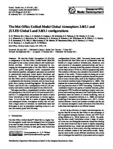
trophic level predators such as sharks, and negligible for the microbes. The reason for diminution of nutrient effects at higher trophic level effects is that nutrients limit the microbial populations whilst increased temperature increases rates of turnover of microbes and hence nutrients, and that there is strong negative feedback on predated populations, which are predated at a higher rate when predator populations increase. 4

The populations of marine species affected by changes in the environment are grouped in seven blocks: microbes (plankton and bacteria), higher level invertebrates (shrimps, crabs, bivalves, etc.), small and medium pelagic fish (herring, mackerel, sand eels, etc.), demersal fish (cod, haddock, etc., but not flatfish), flatfish (sole, plaice etc. excluding skates and rays), sharks (including skate and rays), and a block containing marine mammals and birds. The populations of those species relative to the current temperature and nutrient scenario (baseline) in the four scenarios for temperature and nutrients are shown in Fig. 5. It may be seen that the system is very much nutrient limited, especially in pelagic species (where there is a proportional relationship between nutrients and biomass). In large benthic species and mammals the relationship is less than linear (i.e. a 30 % reduction in biomass for a 50 % reduction in nutrients). The effect of warming is relatively small and greatest for pelagic species and higher Geosci. Model Dev., 9, 947–964, 2016

Discussion/conclusions

Whilst end-to-end modelling, from physics to ecosystem has been characterized as an important procedure in developing an understanding of marine ecosystems, it is one beset by numerous challenges, technical, scientific, and organizational. Couplerlib is designed to address some of the former, which include incompatibilities of system, language, metadata descriptions and terminology, units, spatial and temporal scale, and some of the deepest system problems such as incompatible methods of data storage. In an ideal world we would design end-to-end modelling systems in a top-down co-ordinated manner and the Atlantis model comes closest to this. In other cases some of the technical incompatibilities can be overcome by translating whole models and directly interfacing them to existing models. However, heavyduty model refactoring is expensive and can break the link between development teams working on the core modelling solutions. Couplerlib is proposed as a more workable solution, whose main strength is its ability to operate over difwww.geosci-model-dev.net/9/947/2016/

J. Beecham et al.: Couplerlib: a metadata-driven library ferent coupling strengths from direct coupling to loose coupling via netCDF files. Its main advantage is that the links are made explicit via metadata rather than programming, simple reconciliation of groups and data can be carried out, and it can work across languages and systems including across networks. The main disadvantages of Couplerlib (and of the model coupling approach in general) are it is complex to install and that it still requires interface code to integrate into the models to be coupled. The most difficult parts of this project, where getting the threading interaction between the two models GOTM–ERSEM and EwE, which was a specialist programming task involving waits and signalling between processes, which occurs in the glue layer between Couplerlib and the model code. This is a task that only has to be done once for each modelling tool, so that the majority of model users would not have to alter code. In a large multi-team project, it is likely that the team will include coders and ecological modelling specialist who can work in their specific domain. The technical innovation of the coupling processes and the solutions to the ecological problems that emerged has exposed both technical and ecological issues of reconciling the two models, the key points of which are discussed below. In principle Couplerlib is designed to handle coupling of any groups among models, but in this example only the plankton groups are coupled. The reason for this lies in the effort / benefit ratio, the argument being that plankton groups form the main energy conduits through which environmental changes get translated in to changes in secondary productivity, and poor correspondence between the benthic components of the two North Sea models means a lot of effort would be spent for little marginal gain. Having the dynamics of the benthic components in each model run separately is taken as providing a useful point of comparison. The example coupling links a one-dimensional LTL model calibrated using parameters from the North Sea Oyster Grounds with the HTL food-web model, whose parameters are spatially averaged over the whole North Sea. This discrepancy is related to the more strategic nature of EwE – long-term changes in ecosystem composition versus the more tactical nature of ERSEM – response to environmental transients. While the parameters used to represent each model differ in their degree of spatial specificity, we do not see this giving rise to conceptual or technical issues that cannot be reconciled. First, the Oyster Grounds is a site close to the tidal mixing front that divides summer stratified with the mixed region to the south. Although it simply cannot fully capture the diversity between a mixed site in the southern North Sea and a deep strongly stratified location in the northern North Sea, it is nevertheless representative of the dynamics of a large area of the central North Sea. Second, both models utilize many rate and state parameters from a much wider area of the North Sea or are indeed specified even more generally. The internal consistency of each of the separate models might thus imply that each could be conwww.geosci-model-dev.net/9/947/2016/

959 sidered as rather general representations of the North Sea ecosystem. From a technical point of view, the practical arguments for coupling these non-spatially resolved models are compelling; the coupling allowing proof of concept on the technical methods and early identification of key ecological issues before extending to spatially resolved models. We believe that the main issues have been resolved and plans are in place to tackle coupling spatially resolved models, knowing full well the new issues will emerge, such as capturing the dynamics of annual migrations for some species. On the other hand, running ERSEM as a spatial model and aggregating over space would help scale up the model. Plankton growth in ERSEM is regulated by four elements: carbon (C), whose production depends on light and temperature, nitrogen (N), phosphorous (P), and silicon (Si). With the particular parameterization chosen for the Oyster Ground model, it has been seen that N is not generally limiting, light, as expected, is only limiting during the winter months, and Si and P are more limiting in spring. However, since we have fixed the total amount of these elements and the model is closed, these results are a consequence of our particular choice of initial conditions rather than being a true model prediction. The dynamics of silicon dynamics is more interesting. Particular diatoms, which are more digestible by mesozooplankton, bloom in early spring and then are replaced by the flagellates and dinoflagellates as the Si concentration drops, a result consistent with Broekhuizen et al. (1995). The possible biological consequences of this are discussed by Officer and Ryther (1980). One consequence of the Si dependency of diatom production is that Si is only gradually accumulated as a result of inflow from rivers and thus does not change much from one year to the next, so that the total diatom production level is constant from one year to the next although timing of spring bloom will vary from year to year in relation to temperature and light. There is apparent inter-annual variation between the timing of the growth of the different phytoplankton peaks, the importance of which will depend on the ability of zooplankton to incorporate biomass from the different phytoplankton groups. This single point or average model cannot represent the inter-annual variation in phytoplankton bloom location resulting from inter-annual variation in weather combined with ocean currents. For example, where plankton bloom location varies in space from year to year, the effect on the higher trophic level species will depend on the ability of that species to move with the plankton bloom location. Another issue is that of the spatial pattern of biomass production across the whole of the North Sea, which can vary considerably across time. For example, data used in a metaanalysis by Broekhuizen et al. (1995) showed considerable variation in summer peak omnivorous zooplankton numbers with populations off the Norway coast (box 3 in their paper) having a peak between days 100 and 180, whilst populations off Denmark (box 10) were low until after day 150 and stayed high between day 180 to 270, a late summer bloom. Overall Geosci. Model Dev., 9, 947–964, 2016

960

J. Beecham et al.: Couplerlib: a metadata-driven library Pelagics 1.2 1 0.8

Mammals

Demersal

0.6 0.4 A1B-High Nut.

0.2

B1-High Nut.

0

A1B-Low Nut.

Inverts

Flatfish

Microbes

B1-LowNut.

Sharks

Figure 5. Changes in relative biomass of seven classes of functional groups under differing conditions of warming and nutrient availability (see Table 2 for definitions).

the original ERSEM parameterization placed too much emphasis on the spring diatom bloom as a source of production and so gave a pattern of productivity which did not lead to a stable ecosystem. The current parameterization, which peaks around day 180, gives a better estimate of mean mesozooplankton biomass, even though the nutrient model that gives rise to it requires some refinement to fit to observed levels. There are a number of known divergences from observations for the ERSEM model: for carnivorous zooplankton there is under prediction in winter and too great a rise in spring (avoided by moving this group to EwE); and for microzooplankton there is an over estimate of densities (although this may be as a result of errors in the observations) (Broekhuizen et al., 1995). Modified EwE parameterizations have been made to correct for these: reducing winter metabolism and setting consumption for herring to be very low in winter and adjusting the maintenance cost of herring downwards, in order to prevent this underestimation leading to broader erroneous trophic effects, as a result of erroneous herring deaths. In the long-term improvements to the zooplankton component of ERSEM may remove the need for some of these corrections. In the short term these results raise a number of issues about the dynamics of planktivorous species such as herring. Given the paucity of zooplankton during the winter months, how do they manage to survive over winter? The answers seem to be multifaceted; herring switch prey over the winter months (Blaxter and Hunter, 1982), herring are migratory and may move to extend the season of availability of food (Corten, 2000) and herring do seem to exist in a negative energy balance over winter leading to loss of condition. All these aspects are of potentially

Geosci. Model Dev., 9, 947–964, 2016

great interest for researchers and should be incorporated into future versions of the underlying models. The time frame of the constituent models is critical to their interoperability. This has often been characterized in terms of time step, but reality is much more complex than that. GOTM is a model that makes use of very high-resolution temporal data, to represent the effects of short-term weather conditions and tides, at a temporal resolution that is sub-hourly. The biological component of ERSEM can respond to these changes in a matter of days because some of the functional groups, for example, bacteria and diatoms can respond over this time frame. In the same way the Ecosim model has these components with P / B ratios of 30 s year−1 or more suggesting that the daily time frame is more appropriate for simulation than the default monthly time frame. However, Ecosim is a model that relies on empirical calibration that is usually annual, although some attempts have been made to make seasonal Ecosim models with quarterly recalibration (Althauser, 2003). In the current context it would seem that there is a need for seasonal adjustment of parameter values (especially of P / B ratios, basal metabolic rate and starvation mortality). Data for this calibration are not generally available at high frequency, however. Differences in biomass and productivity between, often quite closely related species vary considerably between the original North Sea Ecosim model and the coupled model. However, both of these results are an encapsulation of a complex spatiotemporal dynamic because there are seasonal fluctuations in the abundance of many of these species. To make a detailed predictive coupled model would require calibration in time and space, ascertaining, for example, the changes in diet composition that occur in time and space. When seasonal www.geosci-model-dev.net/9/947/2016/

J. Beecham et al.: Couplerlib: a metadata-driven library variation in productivity is included (e.g. by coupling models or adding in seasonal forcing), temporal calibration in Ecopath with Ecosim requires consideration of seasonal effects on long-term equilibrium, and given that Ecosim may have multiple equilibria, coupling may cause instability in equilibria in some circumstances. Does short-term behaviour matter when considering longterm environmental change? In terms of the pelagic system the answer would seem very much to be yes. Over-winter survival of everything from small pelagic fish to seabirds seems to depend upon reserves built up in the previous season, and variation in survival and recruitment is generally considered to be influenced by bottom-up constraints on feeding. In the modelling exercise reported here it was found that overwinter survival often depended on sufficiently rapid growth of plankton populations in spring when a fish’s metabolism was increasing. It was necessary to ensure that the forcing functions used to limit winter feeding matched the timing of the spring bloom. Further software development could enable this matching to be automatic. This development could be used to model situations, such as the case of Moroccan sardine populations, where timing between zooplankton peaks and conditions favourable for spawning influences recruitment (Machuo et al., 2009). We can use experimental plankton studies to make a sensitive calibration of planktonic response to short-term meteorological variation, but our ability to explore the effect of climate change on the whole ecosystem, particularly its higher trophic level components, and to predict typical weather in future years is very limited. The addition of a process-oriented model such as GOTM– ERSEM to EwE may allow us to express the relationships between the drivers of change and the consequences. However, the relative insensitivity of EwE to short-term perturbations begs a number of questions as to its suitability in studies on the likely consequences of climate perturbations to the ecosystem. First, the fixed seasonality of Ecosim may not adequately represent the results of shifts in the timing of variable onset events such as plankton blooms, but could be incorporated by adding a run time updated forcing function to the feeding via a plug-in within Ecosim. Second, Ecosim is limited in its ability to represent the effect of environmental variation on transient stages of the life cycle of marine organism such as the pelagic larvae of fish and benthic invertebrates. This is because of the lack of a model of short-term drivers and components for body condition, and the calibration of the multi-stanza model based on a Von Bertalanfy growth curve, which is based on the growth curve of sharks and does not represent larval stages well (Urban, 2002). The North Sea model calibration, consequently, pays little attention to these stages. Recognising such limitations, we are however faced with a practical dilemma; the need for data and modelling tools that help address the pressing research question about how ecosystem respond to change, and the implications for management. The pragmatic route must be

www.geosci-model-dev.net/9/947/2016/

961 to use the modelling capability we have and use it to help learn how to do better in the future. Alongside the issue of time is that of space. For some parameter values there were times of the year when either prey or predators became severely depleted because of availability of prey, but in reality the patchiness of and interconnectedness of areas with different prey levels would lead to rapid recolonization of the area by new predators and prey. An example of spatiotemporal local severe depletion was that of the Bay of Biscay anchovy in 2005 (Borja et al., 2008). To address this, an Ecospace model (the spatial equivalent of Ecosim) can be linked to the ERSEM model within GETM, the spatialized version of GOTM; this will allow us to model the temporal shift of marine organisms in response to the spatiotemporal dynamics of both marine plankton and fishing pressure. However, spatial biogeochemical models require considerable computational resources to run in most practical situations (typically of the order of a week or more time on a cluster for a 100-year run). The single column GOTM– ERSEM model requires about 90 s year−1 to run on an Intel i5 processor, and combined with the integrated front end, makes it much more suitable for exploratory parameterization, teaching, and prototyping than the larger models. The Ecosim model takes under 1 s year−1 to run, it has a time step of 1 day rather than 10 min and has only a single depth layer so that it is calculating less than 1/1000 of the number of time and space elements and Couplerlib is a small proportion of the Ecosim total (less than 10 %), so it is a trivial addition. However, it is less suited to the situation where biological component models such as BFM (biogeochemical flux model; http://bfm-community.eu/ last access: 1 March 2016) are being called every short time step across the managed interface. In this case a more direct coupling method such as FABM (framework for aquatic biogeochemical models; https://sourceforge.net/projects/fabm/; last access: 1 March 2016) (Bruggeman and Bolding, 2014) is more suitable, though this will not work across languages and systems in the same way Couplerlib does. Couplerlib can still be used for initial metadata validation, however. In the realm of biogeochemical modelling there are a number of different models (e.g. Nemo-PISCES, Aumont et al., 2003; Madec et al., 1991; ECOSMO, Schrum et al., 2006; Ecoham, Pätsch and Kühn, 2008), which model the dynamics of plankton in response to changes in the physical environment mediated by physical oceanography. The differences between the model stem from the number of plankton groups and the treatment of the benthos. However, the treatment of the environment as a three-dimensional grid lends itself to a common interface with Ecosim and Ecospace (its twodimensional equivalent) though with a specification of Couplerlib with two-dimensional data elements and appropriate metadata specification. Ultimately, however, the choice of modelling system will depend on the kind of data available and the parameters collected, because model parameterization is a time-consuming and costly part of any modelling Geosci. Model Dev., 9, 947–964, 2016

962 process. The choice of ERSEM for both one-dimensional and three-dimensional modelling is as a result of the use of this model for the North Sea area being examined. There is considerable debate about whether the components of end-to-end models should be simple or complicated. Very often we are faced with models and sub-models that are both over complicated, in the sense that they contain too many parameters and components (Fulton et al., 2003), and over simplistic, in the sense that they contain what can certainly be described as simplifying formulations and may even be seen as dysfunctional formulations (Anderson and Mitra, 2009). The sterility of this debate has been acknowledged in a number of forums (e.g. the WGIPEM ICES working group http://www.ices.dk/community/groups/ Pages/WGIPEM.aspx) along with the general conclusion dating back to William of Occam that things should be as complicated as necessary but no more so. What are needed, therefore, are not so much simple models as simple conclusions that are likely to be robust to uncertain small scale and detailed assumptions and limitations in model formulation. We are a long way off capturing all the physical, biological, and human conditions that will enable us to predict the cod in the North Sea in 50 years, but we at least are starting to have the tools that enable us to integrate important scientific findings within a whole ecosystem context. In conclusion, linking two very different models has produced a system, which is richly expressive of the kinds of interactions of the different functional groups that form pelagic ecosystems and the causes of dynamics, including temperature, nutrient ratios, and biological components of the system. It is not at this stage very precise (Levins, 1966) because it models a spatial area as a single point in space and because of a number of known limitations not just of the underlying ERSEM and EwE models, but also of spatiotemporal variability of marine data. Nevertheless, the linked model represents a considerable advance on verbal arguments because it can demonstrate the likely relative magnitude of these effects in a wider context of nutrient dynamics and marine fishery management. Code availability Source files within this project have been included as follows: – the source files for the standard C++ interface to Couplerlib – the source files for the Managed interface to Couplerlib, which act as a wrapper when called from managed code other than C/C++ (especially Visual Basic from EwE) – the source files for the interface between Couplerlib and EwE – the XML dictionary, and XML specification files for the GOTM/ ERSEM andEwE models Geosci. Model Dev., 9, 947–964, 2016

J. Beecham et al.: Couplerlib: a metadata-driven library – parameter namelists for GOTM and ERSEM. In addition to this, the model will require a complete implementation of the GOTM, ERSEM, and EwE models, and third party libraries for netCDF reading, a complete Python interpreter (2.5 to 2.7) with Numpy, Matplotlib, and PyQt4 together with driving data for GOTM (e.g. meteorological data) and the Access database of the relevant EwE model. This material can be supplied on request but the kind of support needed to commission any non-trivial implementation of an end-to-end model is likely to require considerable time and resources, which can best be provided by third party support.

The Supplement related to this article is available online at doi:10.5194/gmd-9-947-2016-supplement.

Acknowledgements. The authors would like to thank Karsten Bolding for advice on the use of the GOTM model, Mark Platts for help in the preparation of the Ecosim figures, and Piet Ruadij for help on understanding the ERSEM components of the model. Many thanks to Villy Christensen, Carl Waters, Sherman Lai, Joe Buszowski, and Jeroen Steenbeek of the EwE team at UBC Vancouver for their aid during my 2 weeks stay in Vancouver and remote support for the plug-in. This work was funded under the Framework 7, MEECE program (www.meece.eu), Cefas Seedcorn funding, and Defra contract M1202. Useful discussion leading to the development of the model occurred during a workshop of the EasyCo Interreg project (www.project-easy.info). Edited by: R. Marsh

References Althauser, L. L.: An Ecopath/Ecosim analysis of an estuarine food web: Seasonal energy flow and response to River-flow related perturbations, MSC Thesis Louisiana State University and Agricultural and Mechanical College, 2003. Anderson, T. R. and Mitra, A.: Dysfunctionality in ecosystem models: an underrated pitfall?, Prog. Oceanogr., 84, 66–68, 2009. Aumont, O., Maier-Reimer, E., Blain, S., and Pondaven, P.: An ecosystem model of the global ocean including Fe, Si, P co-limitations, Global Biogeochem. Cy., 17, 1060, doi:10.1029/2001GB001745, 2003. Baretta, J. W., Ebanhoh, W., and Ruardij, P.: The European Regional Seas Ecosystem Model (ERSEM) II, J. Sea Res., 38, 229–483, 1997. Berners-Lee, T., Fielding, R. T., and Masinter, L.: Uniform Resource Identifier (URI): Generic Syntax 2005, Internet Society, available at: https://www.rfc-editor.org/rfc/rfc3986.txt (last access: 1 March 2016), 2005.

www.geosci-model-dev.net/9/947/2016/

J. Beecham et al.: Couplerlib: a metadata-driven library Blackford, J. C., Allen, J. I., and Gilbert, F. J.: Ecosystem dynamics at six contrasting sites: a generic modelling study, J. Marine Syst., 52, 191–215, 2004. Blaxter, J. H. S. and Hunter, J. R.: The biology of Clupeoid fishes, Adv. Mar. Biol., 20, 1–223, 1982. Borja, A., Fontán, A., Sáenz, J., and Valencia, V.: Climate, oceanography, and recruitment: the case of the Bay of Biscay Anchovy (Engraulis sicolus), Fish. Oceanogr., 17, 477–493, 2008. Broekhuizen, N., Heath, M. R., Hay, S. J., and Gurney, W. S. C.: Modelling the dynamics of the North Sea’s Mesozooplankton. Netherlands, J. Sea Res., 33, 381–406, 1995. Bruggeman, J. and Bolding, K.: GOTM Graphical User Interface, available at: http://www.gotm.net/index.php?go= software&page=gui/index, 2007. Bruggeman, J. and Bolding, K.: A general framework for aquatic biogeochemical models, Environ. Model. Softw., 61, 249–265, 2014. Burchard, H., Bolding, K., and Villarreal, M. R.: GOTM – a general ocean turbulence model. Theory, applications and test cases, Tech. Rep. EUR 18745 EN, European Commission, 1999. Burchard, H., Bolding, K., Kuhn, W., Meister, A., Neumann, T., and Umlauf, L.: Description of a flexible and extendable physicalbiogeochemical model system for the water column, J. Marine Syst., 61, 180–211, 2006. Chavez, F. P., Ryan, J., Lluch-Cota, S. E., and Ñiquen, M.: From anchovies to sardines and back: multidecadal change in the Pacific Ocean, Science, 299, 217–221, 2003. Christensen, V., Walters, C. J., and Pauly, D.: Ecosim with Ecopath: a user’s guide, November 2005 Edn., Report Fisheries Centre, University of British Columbia, Vancouver, Canada, 2005. Clark, A. and Johnson, N. M.: Scaling of metabolic rate with body mass and temperature in teleost fish, J. Anim. Ecol., 68, 893–905, 1999. Corten, A.: A possible adaptation of herring feeding migrations to a change in timing of the Calanus finmarchicus season in the eastern North Sea, ICES J. Mar. Sci., 57, 1261–1270, 2000. Cushing, D. H.: Towards a science of recruitment in fish populations, in: Excellence in Ecology, edited by: Kinne, O., 7, 175 pp., Ecology Institute, Luhe, Germany, 1996. Daewel, U., Sætre Hjøllo, S., Huret, M., Ji, R., Maar, M., Niiranen, S., Travers-Trolet, M., Peck, M. A., and van de Wolfshaar, K. E.: Predation control of zooplankton dynamics: a review of observations and models ICES J. Mar. Sci., 71, 254–271, 2014. Engelhard, G. H., van der Koij, J., Bell, E. D., Pinnegar, J. K., Blanchard, J. L., Mackinson, S., and Righton, D.: Fishing mortality versus natural predation on diurnally migrating sandeels, Ammodytes marinus, Mar. Ecol. Prog. Ser., 369, 213–227, 2008. Frigstad, H., Andersen, T., Hessen, D. O., Naustvoll, L.-J., Johnsen, T. M., and Bellerby, R. G. J.: Seasonal variation in marine C : N : P stoichiometry: can the composition of seston explain stable Redfield ratios?, Biogeosciences, 8, 2917–2933, doi:10.5194/bg-8-2917-2011, 2011. Fulton, E. A.: Approaches to end to end ecosystem models, J. Marine Syst., 81, 171–183, 2010. Fulton, E. A., Smith, A. D. M., and Johnson, C. R.: Effect of complexity on marine ecosystem models, Marine Ecol. Prog. Ser., 253, 1–6, 2003.

www.geosci-model-dev.net/9/947/2016/

963 Kearney, K. A.: An analysis of marine ecosystem dynamics through development of a coupled physical-biogeochemical-fisheries food web model, PhD Thesis, University of Princetown, 2012. Le Hégaret, P., Whitmer, R., and Wood, L.: Document Object Model, available at: http://www.w3c.org/DOM (last access: 1 March 2016), 2009. Levins, R.: The Strategy of Model Building in Population Biology, Am. Sci., 54, 421–431, 1966. Lewis, K. and Allen, J. I.: Validation of a hydrodynamic-ecosystem model simulation with time-series data collected in the western English Channel, J. Marine Syst., 3, 296–311, 2009. Libralato, S. and Solidoro, C.: Bridging biogeochemical and food web models for an End-to-End representation of marine ecosystem dynamics: The Venice lagoon case study, Ecol. Model., 220, 2960–2971, 2009. Lotze, H. K. H. S., Lenihan, B. J., Bourque, R. H., Bradbury, R. G., Cooke, M. C., Kay, S. M., Kidwell, M., Kirby, C. H., Peterson, J. B., and Jackson, C.: Depletion, Degradation, and Recovery Potential of Estuaries and Coastal Seas, Science, 312, 1806–1809, 2006. Machuo, E., Ettahiri, O., Kifani, S., Benazzouz, A., Makaoui, A., and Demarcq, H.: Environmental control of the recruitment of sardines (Sardina pilchardus) over the western Saharan shelf between 1995 and 2002: a coupled physical / biogeochemical modelling experiment, Fish. Oceanogr., 18, 287–300, 2009. Mackinson, S. and Daskalov, G.: An ecosystem model of the North Sea to support an ecosystem approach to fisheries management: description and parameterisation, Sci Ser. Tech. Rep., Cefas Lowestoft, 142, 196 pp., 2007. Madec, G., Chartier, M., Delecluse, P., and Crépon, M.: A threedimensional numerical study of deep water formation in the Northwestern Mediterranean Sea, J. Phys. Oceanogr., 21, 1349– 1371, 1991. Minto, C., Myers, R. A., and Blanchard, W.: Survival variability and population density in fish populations, Nature, 452, 344–347, 2008. Nakicenovic, N., Alcamo, J., Davis, G., de Vries, B., Fenhann, J., Gaffin, S., Gregory, K., Grubler, A., Jung, T. Y., Kram, T., La Rovere, E. L., Michaelis, L., Mori, S., Morita, T., Pepper, W., Pitcher, H. M., Price, L., Riahi, K., Roehrl, A., Rogner, H.-H., Sankovski, A., Schlesinger, M., Shukla, P., Smith, S. J., Swart, R., van Rooijen, S., Victor, N., and Dadi, Z.: Special Report on Emissions Scenarios : a special report of Working Group III of the Intergovernmental Panel on Climate Change. Cambridge University Press, New York, NY (US), 2000. Officer, C. B. and Ryther, J. H.: The importance of silicon in marine eutrophication, Mar. Ecol. Prog. Ser., 3, 83–91, 1980. Pätsch, J. and Kühn, W.: Nitrogen and carbon cycling in the North Sea and exchange with the North Atlantic – a model study, Part I. Nitrogen budget and fluxes, Cont. Shelf Res., 28, 767–787, 2008. Peterson, P.: F2Py: Fortran to Python Interface Generator, available at: http://cens.ioc.ee/projects/f2py2e/ (last access: 1 March 2016), 2007. Richardson, A. J. and Schoeman, D. S.: Climate impact on plankton ecosystems in the Northeast Atlantic, Science, 305, 1609–1612, 2004. Rose, K. A.: End-to end models for marine ecosystems: Are we on the precipice of a significant advance or just putting lipstick on a pig?, Scientia Marina, 76, 195–201, 2012.

Geosci. Model Dev., 9, 947–964, 2016

964 Rose, K. A., Werner, F. E., Megrey, B. A., Noguchi-Aita, M., Yamanaka, Y., Hay, D. E., Schweigert, J. F., and Foster, M. B.: Simulated herring growth responses in the Northeastern Pacific to historic temperature and zooplankton conditions generated by the 3-dimensional NEMURO nutrient-phytoplanktonzooplankton model, Ecol. Model., 202, 184–195, 2007. Rose, K. A., Allen, J. I., Artioli, Y., Barange, M., Blackford, J., Carlotti, F., Cropp, R., Daewel, U., Edwards, K., Flynn, K., Hill, S. L., HilleRisLambers, R., Huse, G., Mackinson, S., Megrey, B., Moll, A., Rivkin, R., Salihoglu, B., Schrum, C., Shannon, L., Shin, Y.-J., Smith, S. L., Smith C., Solidoro, C., St. John, M., and Zhou, M.: End-To-End Models for the Analysis of Marine Ecosystems: Challenges, Issues, and Next Steps, Marine and Coastal Fisheries: Dynamics, Management, and Ecosystem Science, 2, 115–130, 2010. Rossberg, A. G.: Food webs and biodiversity: Foundations, models, data, Wiley, Chichester, West Sussex, UK, 2013. Schrum, C., Alekseeva, I., and Stjohn, M.: Development of a coupled physical–biological ecosystem model ECOSMOPart I: Model description and validation for the North Sea, J. Marine Syst., 61, 79–99, 2006.

Geosci. Model Dev., 9, 947–964, 2016

J. Beecham et al.: Couplerlib: a metadata-driven library Travers, M., Shin, Y.-J., Jennings, S., and Cury, P.: Towards end-toend models for investigating the effects of climate and fishing in marine ecosystems, Prog. Oceanogr., 75, 751–770, 2007. Travers, M., Shin, Y.-J., Jennings, S., Machu, E., Huggett, J. A., Field, J. G., and Cury, P. M.: Two-way coupling versus one-way forcing of plankton and fish models to predict ecosystem changes in the Benguela, Ecol. Model., 220, 3089–3099, 2009. Urban, H. J.: Modeling growth of different developmental stages in bivalves, Mar. Ecol. Prog. Ser., 238, 109–114, 2002. van der Molen, J., Aldridge, J. N., Coughlan, C., Parker, E. R., Stephens, D., and Ruardij, P.: Modelling marine ecosystem response to climate change and trawling in the North Sea, Biogeochemistry, 113, 213–236, 2012. Vichi, M., Oddo, P., Zavatarelli, M., Coluccelli, A., Coppini, G., Celio, M., Fonda Umani, S., and Pinardi, N.: Calibration and validation of a one-dimensional complex marine biogeochemical flux model in different areas of the northern Adriatic shelf, Ann. Geophys., 21, 413–436, doi:10.5194/angeo-21-413-2003, 2003.

www.geosci-model-dev.net/9/947/2016/