Sep 21, 2015 - In this article, an extension to the open-source tools. PyFMI and Assimulo is .... the aggregated system is simply to call the RHS-function of each ...
Coupling Model Exchange FMUs for Aggregated Simulation by Open Source Tools Pukashawar Pannu1 1 Centre
Christian Andersson1,2
Johan Åkesson2
for Mathematical Sciences, Lund University, Sweden 2 Modelon AB, Sweden
Abstract
The dynamical models considered here can be described as,
The Functional Mock-up Interface standard allows to generate stand-alone sub-systems which can be simulated and verified individually. In this paper we present a design of a model aggregation which allows to simulate several Functional Mock-up Units as a coupled model. The formulation is based on Assimulo as a numerical integration environment. Assimulo problem classes are extended to a class for aggregated problems which collects information provided by the Functional Mockup Units through the tool PyFMI together with Python based problem classes defined by Assimulo. This allows to set-up test environments of complex models composed of several sub-systems. Keywords: FMI, Jacobian, Algebraic loops, Events, Model Exchange 2.0, Assimulo
1 Introduction
Claus Führer1
x¯˙ = f¯(x, ¯ u) ¯ y¯ = g( ¯ x, ¯ u) ¯
(1a) (1b)
where x¯ represents the states, u¯ the input signal and y¯ the output, consistent with the FMI. Commonly, a full system model is represented by several stand-alone sub-systems coupled together by coupling equations to a model for a global system. This results in the following general system description, x˙ = f (x, u, w) y = g(x, u, w) u = c(y, w)
(2a) (2b) (2c)
where x represents the combined states from the separate models. The local inputs for the ith model, u¯[i] , has here been separated into two vectors, u¯[i] = [uˆ[i] , wˆ [i] ], and subsequently combined into the global vectors (for N models), u = [uˆ[1] , . . . , uˆ[N] ] and w = [wˆ [1] , . . . , wˆ [N] ]. This as to separate between inputs determined by the coupling, u, and external inputs acting on the coupled system, w. In general the external inputs can not only influence the model behaviour directly but also the coupling, Eq (2c), which is highlighted in Section 3. When solving a coupled system, an approach is cosimulation as is explored in (Andersson, 2013) where the systems have their own integrator and the focus is on communication between systems. In this paper however, the focus is on coupling model exchange FMUs under a single solver.
The Functional Mock-up Interface (FMI) (Blochwitz et al., 2012) has gained momentum in simulation of dynamical systems and in exchanging dynamic simulation models between tools. The standard has proven to be highly successful as it fills a gap where there were costly custom integrations before. The open source tools PyFMI 1 together with Assimulo (Andersson et al., 2015) provide a solid foundation for performing simulations and experiments on single Functional Mock-up Units (FMUs). A key feature that is currently lacking is the ability to easily simulate coupled systems and thus fully taking advantage of the standard. In this article, an extension to the open-source tools PyFMI and Assimulo is presented that allows for simulation of coupled model exchange FMUs following the 2 Concept FMI 2.0 standard. The extension enables coupling of FMUs and models written directly in Python to a so- The idea is to take N coupled sub-systems, either FMUs or Python models, and aggregate them into a single syscalled aggregated model. tem and treating the final full system as any other model. 1 http://www.pyfmi.org PyFMI - Version 2.1. Accessed, In order to facilitate the general description of a subsystem, as is defined in FMI, for the aggregated system, 2015-05-18 DOI 10.3384/ecp15118903
Proceedings of the 11th International Modelica Conference September 21-23, 2015, Versailles, France
903
Coupling Model Exchange FMUs for Aggregated Simulation by Open Source Tools
care needs to be considered in how for example the Jacobian is defined. The Jacobian is a necessity when using implicit methods for solving the resulting system and is discussed in Section 2.3. Additionally, the events for each sub-system and external events need to be considered, discussed in Section 2.2, as well as algebraic loops which can occur due to the coupling, Section 2.4. Now, looking at N sub-systems, [1] [1] [1] [1] [1] x˙¯1 = f¯1 (x¯1 , uˆ1 , wˆ 1 ) [1]
[1]
[1]
[1]
[1]
[1]
[1]
y¯1 = g¯1 (x¯1 , uˆ1 , wˆ 1 ) [1]
.. .
(3a)
• RHS (Right-Hand-Side) function of aggregation.
(3b)
• Coupling handling.
[N] [N] [N] [N] [N] x¯˙N = f¯N (x¯N , uˆN , wˆ N )
(4a)
[N] y¯N [N] u¯N
(4b)
=
[N] [N] [N] [N] g¯N (x¯N , uˆN , wˆ N ) [N] [N] c¯N (y¯[N] , wˆ N )
and the resulting aggregated system, [1] [1] [1] [1] f¯1 (x¯1 , uˆ1 , wˆ 1 ) .. x˙ = f (x, u, w) = . [N] [N] [N] [N] f¯1 (x¯1 , uˆ1 , wˆ 1 ) [1] [1] [1] [1] g¯N (x¯N , uˆN , wˆ N ) .. y = g(x, u, w) = .
[N]
[N]
• Aggregated states.
(3c) Through PyFMI there exists already a wrapper interface that can load an FMU ME 2.0 and integrate it using Assimulo. When instantiating the AggregatedProblem class a list of FMUs is provided from which the initial states are easily accessible and aggregated,
u¯1 = c¯1 (y¯[1] , wˆ 1 )
=
to one large problem that can be integrated using one of Assimulos available solvers, called AggregatedProblem. For simplicity an already existing problem class, ExplicitProblem, was extended to handle the aggregation. To define an aggregated problem class some basic data is required:
[N]
f o r model i n m o d e l s : aggregated_x0 a g g r e g a t e model.x0
The crucial part of the aggregated problem class is how (4c) to handle the right hand side function. The first major difference between an aggregated problem and an Assimulo problem is the presence of couplings. For each call to the RHS, coupling terms must be up to date. The condition can be satisfied by updating the coupling rela(5a) tions within the RHS-function. Since the separate problem classes already have an RHS-function structure, computing the RHS-function of the aggregated system is simply to call the RHS-function (5b) of each sub-system,
[N]
g¯N (x¯N , uˆN , wˆ N ) [1] [1] [1] c¯1 (y¯ , wˆ 1 ) .. u = c(y, w) = .
(5c)
set_connections ( ) f o r model i n m o d e l s : aggregated_rhs aggregate model.rhs
Coupling handling is done in set_connections(). For [A] simple cases when for example system A input u2 needs The vectors x, y, u and w of the aggregated system are inputs from system B output y[B] , the function simply sets 4 defined as: [B] [A] u2 = y4 . However, this is not always the case which is [1] further discussed in Section 2.4. [1] [1] [1] wˆ 1 uˆ1 y¯1 x¯1 For implicit solvers a Jacobian is required and must be .. .. .. .. x = . , y = . , u = . , w = . provided by AggregatedProblem. More advanced [N] [N] [N] [N] models require AggregatedProblem to take into acuˆn y¯N wˆ N x¯N count events and algebraic loops. The three mentioned topics are affected by aggregation and are discussed in 2.1 Aggregated Problem the following sections. Using the open-source tools PyFMI together with Assimulo, an FMU can be accessed from Python 2.2 Events together with being solved using solvers available in Assimulo. With this in mind two Assimulo Many models include discontinuities. One way of inproblem classes have been worked on. One that tegrating such systems is by using events (Eich-Soelner creates an input/output problem structure called and Führer, 1998) which requires that a set of event inExplicitProblemModel. The other aggregates dicators are monitored during the integration. The inteseveral FMUs, or ExplicitProblemModels, gration is interrupted when conditions on the event indi[N] [N] c¯N (y¯[N] , wˆ N )
904
Proceedings of the 11th International Modelica Conference September 21-23, 2015, Versailles, France
DOI 10.3384/ecp15118903
Poster Session
cators are violated and the event (discontinuity) is appropriately handled, finally the integration is restarted. Most of the solvers available in Assimulo have this functionality (Fredriksson et al., 2014). The aggregated problem can access event indicators of an FMU. When asked for event indicators by an Assimulo solver the AggregatedProblem combines all event indicators from the sub-systems and hands them to the solver. Once an event has been detected and the integration stopped, the problem class identifies the triggered event and calls the corresponding sub-system’s event handling. Another type of events in FMUs are time events, which are known at the start of a simulation. They split up the integration into segments by setting up end times for the simulation at which point an event is handled (Andersson, 2013). This could be, for instance, a force periodically applied to the system. It is up to the aggregated system to search through all sub-systems for the closest time event to define the end time of the next integration segment and handle the event. From the Assimulo problem design it is simple to add events to a problem. For the aggregated problem, adding of events would be to add external events to a coupled system. Events can not only be provided through the sub-systems but also through how the system is coupled. Consider a pendulum with no knowledge of its surroundings. Now, in the system model the pendulum is positioned such that its degree of freedom is limited by for instance positioning close to a wall. The limitation can be considered as an external event that needs to be taken into account. In the problem formulation this is easily done by providing extra sets of event indicators for the integrator to monitor.
The term
∂y ∂x
is found by differentiating Eq (7b): ∂y ∂g ∂g ∂c ∂y = + ∂x ∂x ∂c ∂y ∂x
Solving for
∂y ∂x
gives: � � ∂y ∂ g ∂ c −1 ∂ g = I− ∂x ∂c ∂y ∂x
x˙ = f (x, u, w) y = g(x, u, w) u = c(y, w) Inserting Eq (6c) into Eq (6a) and Eq (6b) gives: x˙ = f (x, c(y), w) y = g(x, c(y), w) Differentiating Eq (7a) with respect to x yields: J= DOI 10.3384/ecp15118903
∂ f ∂ f ∂c ∂y + ∂x ∂c ∂y ∂x
(10)
Resulting in the Jacobian: J=
� � ∂ f ∂ f ∂c ∂ g ∂ c −1 ∂ g + I− ∂x ∂c ∂y ∂c ∂y ∂x
(11)
For the system to be solvable there is necessary condition that (I − ∂∂ gc ∂∂ cy ) is non singular. The ∂∂ gc term handles the coupling relations and ∂∂ cy the sub-system feed-through terms. With FMI 2.0 models have an option to provide directional derivatives. In case they are provided AggregatedProblem uses directional derivatives to approximate the aggregated Jacobian matrix. If directional derivatives are unavailable a forward difference scheme is applied. The same applies for non-FMI models.
2.4 Algebraic Loops When a system contains feed-through, i.e. when the partial derivative of Eq (6b) with respect to u is not the zero matrix, then, in general, an equation system needs to be solved to maintain consistent input and output values satisfying, y = g(x, u, w) u = c(y, w).
2.3 Jacobian When solving an ODE the Jacobian can be explicitly provided or numerically approximated. For an uncoupled input/output system where the inputs are only time de¯ pendent the Jacobian, ∂∂ xf¯ , is computed. When looking at a coupled system the dynamic changes. Due to coupling some input terms are state dependent instead of time dependent as in the uncoupled case. Consider the coupled system,
(9)
(12a) (12b)
By rewriting Eq (12a) to, y − g(x, c(y, w), w) = 0
(13)
the algebraic loop can be solved by an iterative method. AggregatedProblem creates a residual function of the left-hand-side of Eq (13) and uses the Kinsol solver in Assimulo to solve the problem. Kinsol is a non(6a) linear algebraic equation solver, part of the SUNDIALS suite (Hindmarsh et al., 2005). When the outputs are (6b) known, Eq (12b) is used to update the inputs. (6c)
2.5 Workflow (7a) The simulation flow of coupled systems using the aggre(7b) gated problem class and an Assimulo solver is illustrated in Figure 1. The simulation flow is essentially equivalent to that of simulating an ODE with Assimulo, how(8) ever, some nodes are affected by aggregation and these are coloured blue in the figure.
Proceedings of the 11th International Modelica Conference September 21-23, 2015, Versailles, France
905
Coupling Model Exchange FMUs for Aggregated Simulation by Open Source Tools
the pendulum’s pivot. The inputs are forces, u¯2 and u¯3 , acting on the body’s center and an acceleration, u¯1 due to a forced motion of the pivot. The outputs, y, ¯ are the positions. In order to couple two pendula, i = [1, 2], the input vector is split for each pendulum into external excitations and inputs determined by the coupling, [i]
[i]
[i]
u¯[i] = [ u¯1 , u¯2 , u¯3 ]. |{z} | {z } wˆ [i]
(15)
uˆ[i]
The two pendula are coupled by a linear spring which is determined by the equation, u = c(y, w), [1] [1] [2] y¯1 − a + w1 − (y¯1 − b − w2 ) uˆ2 [1] [1] [2] y¯2 − y¯2 uˆ3 [2] = k (16) [2] uˆ2 −(y¯[1] − a + w − ( y ¯ − b − w )) 1 2 1 1 [1]
[2]
uˆ3
Figure 1. Assimulo simulation flow of coupled systems using FMUs, Assimulo problems and the aggregated problem class. The blue color represents nodes that are affected by aggregation.
3 Examples In this section, the proposed framework is demonstrated. The ability to couple model exchange FMUs is shown together with coupling of FMUs with models directly defined in Python. Additionally, simulation of coupled models with externally defined events is demonstrated.
|
[2]
−(y¯2 − y¯2 ) {z =:ρ
}
where k is the stiffness ratio. Variable a represents the pivot points x-coordinate of the left pendulum and b the point of the right pendulum. The external input vector is, w = [w1 , w2 , wˆ [1] , wˆ [2] ].
(17)
The setup is shown in Figure 2. As previously mentioned, it is necessary to include the external inputs into the coupling as is made evident in this example. Note also, that in this example wˆ [i] has to be chosen as w¨ [i] .
3.1 Coupled Pendula This example demonstrates how two FMUs, each describing a pendulum, are coupled to an aggregated model. The full system consists of two pendula coupled by a force and excited by two inputs acting on the pivots. The pendulum, with mass 1 kg and length 1 m, is described by, x¯˙1 = x¯3 x˙¯2 = x¯4 x˙¯3 = u¯1 − 2x¯1 λ + u¯2 x˙¯4 = −g − 2x¯2 λ + u¯3
(14a) Figure 2. Two pendulums coupled via a spring. (14b) The pendulum is modelled in the Modelica language (14c) and using the open-source tool JModelica.org (Åkesson (14d) et al., 2010) the Modelica model is compiled into an 0 = x¯12 + x¯22 − 1 (14e) FMU. The tool is responsible for transforming the peny¯1 = x¯1 (14f) dulum which is described as a DAE of index 3 into an y¯2 = x¯2 (14g) ODE that FMI supports. The aggregated system was integrated using Assimulo where x¯1 , x¯2 are positions and x¯3 , x¯4 velocities relative to CVode solver with tolerances atol = rtol = 10−8 for 5 906
Proceedings of the 11th International Modelica Conference September 21-23, 2015, Versailles, France
DOI 10.3384/ecp15118903
Poster Session
seconds and the Jacobian approximated with forward dif- where g is gravitational acceleration, x¯1 is angular disferences. Initital conditions for the system, placement with respect to the pivot point, x¯2 angular velocity. The inputs u¯2 and u¯3 are forces acting on the bob [1] x¯1 = 1 (18) horizontally and vertically respectively. u¯1 is an input [1] x¯2 = 0 (19) of acceleration due to a forced motion of the pivot. The output, y¯1 , is the angular displacement. [2] x¯1 = −1 (20) Similarly to the example described in Section 3.1 the input vector is split into external excitations and inputs [2] x¯2 = 0 (21) by coupling. note that the initial conditions are from the reference [i] [i] [i] (23) u¯[i] = [ u¯1 , u¯2 , u¯3 ]. point of each pendulums pivot. The pivot points are lo|{z} | {z } cated at (−2, 0) for the left pendulum and (2, 0) for the wˆ [i] uˆ[i] pendulum to the right. As external forces acting on the pivots the sin(t) function was chosen. Stiffness ratio of The linear spring coupling the two pendulas is determined by, the spring is set to k = 1.0 N/m. As reference a monolithic model of the system was [1] [2] [1] (sin(y¯1 ) − a + w1 ) − (sin(y¯1 ) − b − w2 ) uˆ2 created in Modelica and simulated in Dymola (Dassault [1] [2] [1] Systèmes, 2016) using the solver Dassl with tolerance (−cos(y¯1 ) − (−cos(y¯1 )) uˆ3 −12 = k [1] [2] tol = 10 . Error of both pendulums x, y positions is [2] −((sin(y¯1 ) − a − w1 ) − (sin(y¯1 ) − b − w2 )) uˆ2 presented in Figure 3 in log-scale. [1] [2] [2] −((−cos(y¯1 ) − (−cos(y¯1 ))) uˆ3 {z } | 10-4
Error of x, y Positions of FMU Coupled Pendula Problem
=:ρ
(24)
10-5
where k is the stiffness ratio. Variables a and b represent the pivot points x-coordinate for the left-hand-side and right-hand-side pendulas respectively. The external input vector is, u1 = [w1 , w2 , wˆ [1] , wˆ[2] ]. (25)
10-6 10-7 Error
10-8 10-9
10-10 10-11
x1[1]
10-12
x2[1]
As with example in Section 3.1, wˆ [i] has to be chosen as w¨ [i] . x 10-13 x Initial conditions for the aggregated system were cho10-14 0 1 4 5 2 3 sen for the pendulas to mirror each other with angles π2 time (s) and − π2 for the left and right pendulas and zero initial Figure 3. Error of x, y positions of aggregated coupled pen- angular velocity. [2] 1 [2] 2
dulum described in Section 3.1, simulated with CVode with [i] atol = rtol = 10−8 for 5 seconds. x1 denotes the x-coordinate [i] x2
and the y of model i. Model [1] is the pendulum to the left and [2] the one to the right.
3.2 Coupled Pendula with Different Model Types
π 2 [1] x¯2 = 0 [1]
x¯1 =
π [2] x¯1 = − 2 [2] x¯2 = 0
(26a) (26b) (26c) (26d)
As external force exciting the pendula pivots a sin(t) signal was chosen and the springs stiffness ratio k = 1.0 N/m. The aggregated system was integrated using the CVode solver in the Assimulo package with tolerances, atol = rtol = 10−8 for a time of 5 seconds and the Jacobian approximated using forward differences. Results were then compared to a reference where the coupled pendulas were modelled as a monolithic system in Modelica and simulated with Dassl in Dymola using toler(22a) ance tol = 10−12 . Figure 4 shows the error in log-scale (22b) of the angle x¯[1] of all three systems compared to the con1 (22c) trol. The same plot for angle x¯[2] is shown in Figure 5. 1
Three aggregated systems of coupled pendulas were modelled and compared to a monolithic reference model. The first system built by two FMU models modelled in Modelica and compiled with JModelica.org. The second by two Assimulo models and the third with the left pendulum as an Assimulo model and the right pendulum as an FMU. For this example the pendulums were modelled as ODEs in polar coordinates with unit mass and length, x˙¯1 = x¯2 x˙¯2 = (−g + u¯3 )sin(x¯1 ) + (u¯2 + u¯1 )cos(x¯1 ) y¯1 = x¯1 DOI 10.3384/ecp15118903
Proceedings of the 11th International Modelica Conference September 21-23, 2015, Versailles, France
907
Coupling Model Exchange FMUs for Aggregated Simulation by Open Source Tools
Angle x1[1] Error of Coupled Pendula System
1.0 Displacement in x-coord. with respect to pivot point
10-5 10-6
Error
10-7 10-8 10-9 10-10 10-11 0
1
Coupled FMUs Coupled Assimulo Problems Mixed FMUs and Assimulo Problems
2
time (s)
4
3
[1]
Figure 4. Error of angle x1 of aggregated FMU, Assimulo and mixed systems, simulated for 5 seconds with tolerances atol = rtol = 10−8 with CVode solver in Assimulo package. 10-5
x1[1]
0.5
wall[1] x1[2]
wall[2]
1
2
time (s)
3
4
5
Figure 6. Shows the x-coordinate displacement, with respect to their own pivots, of the pendulums [1], to the left, and [2], to the right, has they hit a wall. The horizontal lines represent walls blocking each pendulums path.
[1]
the bobs x-coordinate reaches x¯1 = 0 with respect to its pivot. The right-hand-side pendulum wall is placed slightly to the right of its pivot and the bob impacts the [2] wall when its x-coordinate reaches x¯1 = 0.3 with respect to its pivot. Initial conditions and parameters are the same as for the example described in Section 3.1.
10-7 Error
0.0
Angle x1[2] Error of Coupled Pendula System
10-6
10-8 10-9
10-10 10-11 10-12 0
0.5
1.0 0
5
x Coordinates of Coupled Pendulums with Impact on Walls
1
Coupled FMUs Coupled Assimulo Problems Mixed FMUs and Assimulo Problems
2
time (s)
4
3
The aggregated system was integrated with the CVode solver with tolerances atol = rtol = 10−8 for 5 seconds. Figure 6 shows the x-coordinate displacement with respect to each pendulums pivot. The two horizontal lines represent each pendulums respective walls.
5
[2]
Figure 5. Error of angle x1 of aggregated FMU, Assimulo and mixed systems, simulated for 5 seconds with tolerances atol = rtol = 10−8 with CVode solver in Assimulo package.
4 Conclusion 3.3 Coupled Pendula Impact on Wall The aggregated system constructed with two FMUs in Section 3.1 is here reused with the addition of discontinuities as two walls are externally placed in the path of the two pendulums’ swinging motion. One wall for each pendulum. This as to highlight the possiblity of externally adding state events to the coupled problem. Also the external forces acting on the pivots have been removed. When the bob hits the wall a discontinuity occurs. This is handled by defining event indicators that trigger an event when the impact occurs. Event indicators are defined as zero-crossings as, [i]
event [i] = wall [i] − x¯1
(27)
where wall [i] is the x-coordinate of the wall blocking pendulum [i]. The impact itself is elastic and the event handling is done by simply reversing the velocity of the bob. For the pendulum to the left a wall is placed directly below the pivot point and the impact occurs when 908
In this paper, a framework has been presented for simulation of coupled systems by aggregation. Care needs to be taken when a coupled system contains feed-through as an equation system needs to be solved in order to compute the derivatives of the system. This puts a condition on the sub-system feed-through terms that also presents itself when computing the Jacobian. The sub-system events are handled by aggregation. A benefit of this approach is that events from all subsystems together with external events can be monitored at once and handled through the aggregated system. Example described in Section 3.3 shows that external events can be added to an aggregated coupled system. The FMI has all functionality needed to carry out the presented scheme. By combining the discussed ideas with Assimulo and allowing direct coupling of FMUs and Python based problems one gets a flexible and powerful environment for solving coupled dynamical problems.
Proceedings of the 11th International Modelica Conference September 21-23, 2015, Versailles, France
DOI 10.3384/ecp15118903
Poster Session
References Christian Andersson. A Software Framework for Implementation and Evaluation of Co-Simulation Algorithms. Licentiate thesis, Centre for Mathematical Sciences, Lund University, Lund, Sweden, 2013. Christian Andersson, Claus Führer, and Johan Åkesson. Assimulo: A unified framework for ode solvers. Math. Comput. Simulat., 2015. doi:10.1016/j.matcom.2015.04.007. In press. Torsten Blochwitz, Martin Otter, Johan Åkesson, Martin Arnold, Christoph Clauss, Hilding Elmqvist, Markus Friedrich, Andreas Junghanns, Jakob Mauss, Dietmar Neumerkel, Hans Olsson, and Antoine Viel. Functional mockup interface 2.0: The standard for tool independent exchange of simulation models. In In 9th International Modelica Conference 2012. Modelica Association, 2012. Dassault Systèmes. Dymola - Multi-Engineering Modeling and Simulation - Version 2016. http://www.dymola. com/, 2016. Accessed: 2015-08-01. Edda Eich-Soelner and Claus Führer. Numerical Methods in Multibody Dynamics. European Consortium for Mathematics in Industry (ECMI). Teubner, 1998. ISBN 3-519-026015. Emil Fredriksson, Christian Andersson, and Johan Åkesson. Discontinuities handled with events in Assimulo. In Hubertus Tummescheit and Karl-Erik Årzén, editors, Proceedings of the 10th International Modelica Conference, number 96 in Linköping Electronic Conference Proceedings, pages 827–836. Linköping University Electronic Press, Linköpings universitet, 2014. URL http://dx.doi. org/10.3384/ECP14096827. Alan C. Hindmarsh, Peter N. Brown, Keith E. Grant, Steven L. Lee, Radu Serban, Dan E. Shumaker, and Carol S. Woodward. Sundials: Suite of nonlinear and differential/algebraic equation solvers. ACM Trans. Math. Softw., 31(3):363–396, September 2005. ISSN 0098-3500. doi:10.1145/1089014.1089020. Johan Åkesson, Karl-Erik Årzén, Magnus Gäfvert, Tove Bergdahl, and Hubertus Tummescheit. Modeling and optimization with Optimica and JModelica.org—languages and tools for solving large-scale dynamic optimization problem. Comput. Chem. Eng., 34(11):1737–1749, November 2010. doi:http://dx.doi.org/10.1016/j.compchemeng.2009.11.011.
DOI 10.3384/ecp15118903
Proceedings of the 11th International Modelica Conference September 21-23, 2015, Versailles, France
909