Cournot Equilibrium Calculation in Power Networks

1

Cournot Equilibrium Calculation in Power Networks: An Optimization Approach with Price Response Computation Julián Barquín, Member, IEEE, and Miguel Vázquez



Abstract– Since deregulated power markets are very often oligopolistic ones, efficient models that are able to describe strategic behavior of firms must be developed. In particular, transmission constraints can easily increase the opportunities of market players to exercise market power. This paper presents a model that describes the firms strategic interaction, based on Nash-Cournot equilibrium, when the power network is taken into account. Specifically, this paper introduces a new iterative algorithm, that explicitly considers how the production at a certain bus affects the whole network, and consequently models the opportunities for the firms of exercising market power, taking into account their ability to influence the composition of the set of constrained lines. The theoretical basis of the method as well as a case study based on the Central European network is included. Keywords: Power system economics, interconnected power systems, game theory, oligopoly models, transmission.

I. INTRODUCTION Nowadays it is widely accepted that most electricity markets cannot be modeled under the perfect competition assumption. Therefore, traditional methods to describe electricity markets that assume perfect markets [14], are of limited use. In the case of oligopolistic competition, NashCournot equilibrium is the most popular type of game used to model the interaction between strategic generators (see for instance reviews in [9], [8], [1]). Even if the forecasting capability of these models is questioned, they are useful for gaining insights into the firms’ strategic behavior as they allow for comparisons between different market scenarios. Model differences are due to different assumptions about market mechanisms and about the behavior of the market participants involved, and because of the methods used to solve them. A preliminary, and yet popular, approach to model oligopolistic markets is to disregard the transmission network. There are a number of models that are able to compute more or less sophisticated market equilibria in single-bus networks (see for instance [2], [13], [10]), using different methodologies. However, disregarding the power network is not always suitable mainly because the existence of the network adds opportunities to exercise market power. For instance, J. Barquín and M. Vázquez are with the Technological Research Institute [Instituto de Investigación Tecnológica (IIT)] Universidad Pontificia Comillas, Madrid. e-mail: [email protected], [email protected]

congestion in one or more lines may isolate certain subsets of nodes so that supply to those nodes is effectively restricted to a relatively small subset of producers (see for instance [12]). Then, there will be increased market power, since it is relatively easy for these producers to increase prices in the isolated area by withholding power, independently of the competitiveness of the whole system. We will model the operation of the network as an integrated model, with joint optimization. Although in the regulatory practice several other market mechanisms have been implemented that do not optimize the whole network at the same time (countertrading, explicit auctions...), we will focus on price simulation and thus we will assume that the network management is perfectly efficient. However, models similar to ours could be used to simulate the market under different regulatory solutions (see for instance [7]). Concerning network flows, we use linearized load flow to account for Kirchhoff’s laws including loop flows. This contrasts with early models of power networks which disregarded the Kirchhoff voltage law (transportation models) [11]. However, because energy flow cannot be confined in a certain path, some effects, such as loop flows, prompt more recent models to consider both laws, usually by a linearized load flow. Prior network representations complicate the problem of determining how the strategic producers will react to changes in a certain nodal (or zonal) price caused by changes in their output wherever they are located. When a single-bus network is assumed this price response is just the demand elasticity in the Cournot model; but if the power network is taken into account, the price sensitivity is the demand elasticity faced by the producers, which depends on the set of congested lines. So when the firms decide their output, they must anticipate which lines will be congested after the market clearing in order to anticipate how their production will affect the prices. One way of tackling this problem is within the leaderfollower framework. The problem can be stated as a two-stage game, where first the firms allocate their output and submit their bids to the central auctioneer (leaders) and then the central auctioneer clears the market, provided the bids of the firms (follower). When this two-stage model is considered (for instance [12], [5]), each firm (each leader) faces the problem of maximizing its profit subject to its own constraints (maximum and minimum output, etc) and the first-order

2

conditions of the central auctioneer problem1. The solution of the set of equations provided by each firm’s problem is the Nash-Cournot game solution2, which takes into account the ability of the producers to anticipate how their output affects the network prices. Unfortunately, when the transmission network is taken into account by means of a DC load flow, a pure strategies equilibrium for such a game may not exist or may be not unique [3], [9], since optimality conditions of the auctioneer problem considered as constraints of the firms’ profit maximization result in a non-convex feasible region. Another proposal to cope with the problem is to assume some conjectured reaction of the firms to the decisions of the transmission system operator, facilitating the convexity of the feasible region (and in addition the computational efficiency), while still playing a quantity game against other firms when deciding their output. This is the case of [6] and [4], which assume the reactions of the firms to the decisions of the transmission system operator as exogenous parameters regardless of the distribution of the flows in the network (in [6] the conjecture is no reaction, i.e. firms are price-takers with respect to transmission prices). This paper proposes a novel way to obtain the price sensitivity avoiding the statement of a two-stage game. It is achieved by means of an iterative algorithm which can be thought of as follows: the firms assume that the central auctioneer will decide that a certain set of transmission lines will be congested and with that assumption decide their output. If the assumption is consistent with the realized congested lines, then the solution is a Nash-Cournot equilibrium. The firms’ assumptions about congested lines gives the price response of the firms, so that each iteration can be understood to be a conjectured price response of the firms (along the same lines as [6] and [4]). However, the iterative procedure we introduce in this paper may be viewed as a way of selecting the firms’ reactions to the power network constraints consistent with the central auctioneer behavior, and thus of foreseeing the auctioneer’s reactions to the firms’ bids. In addition, the players’ profit maximization follows the work in [2]. Since it is based on a quadratic optimization3 it can take advantage of a very well-developed theoretical corpus as well as very powerful algorithms and software. So this model can deal with real-size systems with a reasonable amount of computational effort, less than that of complementarity approaches. An in-depth comparison between the three above approaches can be found in [1]. Nonetheless the convergence of the algorithm is not always assured. The specified game may have no pure strategies equilibrium so the algorithm will not converge. Also, since we calculate the price derivatives by assuming a certain set of congested lines in the system, we do not consider points where the price derivative is 1 This kind of problem is called a mathematical program with equilibrium constraints, MPEC. 2 Finding the equilibrium among several MPECs, one per firm considered, is called an equilibrium problem with equilibrium constraints, EPEC. 3 Instead of the more usual complementarity approaches, (MCP or variational inequality problem).

not defined. These non-smooth points of the profit function cannot be taken into account by the algorithm preventing its convergence. However, in such cases multiple Nash-Cournot equilibria (even a continuum of equilibria) may exist [3]. This case is not theoretically closed, but a rough discussion can be found in Section V. Section II provides a general scheme of the proposed iterative algorithm, and a more detailed statement of the assumptions considered. Section III describes generators and auctioneer modeling. The model requires the computation of nodal (zonal) price sensitivities to generation changes, which is addressed in Section IV. Section V shows a complete sight of the algorithm. A stylized case study based on a real-world network is analyzed in Section VI. Finally, our conclusions are stated. Some mathematical proofs are collected in the Appendices. II. GENERAL SCHEME A single-period, purely thermal, model is considered. It would not be difficult to generalize to a multi-period model, including intertemporal constraints as the hydro constraints following the work in [2]. However, as the this study focuses on the network-related effects, a simplified single-period model has been considered. Each generating unit gu (belonging to firm g ) is characterized max min Pgu , Pgu

by

a

maximum

and

minimum

output,

respectively, and a convex cost function

 

Cgu  Cgu Pgu

of the power output Pgu . Generators (also

called firms or utilities) behave as Cournot oligopolists, i.e., they set their production in order to maximize their profit, assuming known demand curves and fixed competitors’ outputs. Furthermore, there may be units belonging to several generators at each bus, and each generator may have units located at several buses. Linear demand curves at each bus are considered. Each transmission line is characterized by an admittance and a maximum flow. DC power flow equations are assumed, and no losses are considered. Thus, the dispatch problem of each of the generators in the market is a profit maximization one, where a critical factor that each generator must take into account is how system prices change when the output of each of its units is modified. Considering these effects is not trivial. Changes in the production of a certain unit have an effect not only on the price of the bus where the generator is located, but on the whole network. These sensitivities are not constant. Due to the linear demand equations and the DC load flow formulation (see Section V), they depend on the set of constrained lines in the network (hereinafter, we will refer to this set as network state). Therefore, price sensitivities cannot be computed without an assumption on the behavior of the other generators. To obtain a Nash-Cournot equilibrium this assumption must be consistent, that is, the network state assumed when deciding

3

the output of each unit must be the same one as the network state obtained after clearing the market. An iterative algorithm is proposed in order to find an equilibrium. First, a network state is assumed. Then, sensitivities are computed, and the dispatch (which specifies the solution of the generators’ profit maximization under the assumed prices sensitivities) is solved, finding the new network state. If it coincides with the network state previously assumed, then the algorithm ends; if not, new sensitivities are computed and the whole procedure iterates again. Network state Dispatch problem

Sensitivities computation



belonging to generator g. One vector is defined for each firm g.  Pg1  Pg       F is the matrix, obtained from the admittance data, relating flows and voltage phases: f  F θ .  M is the buses-lines incidence matrix. M  i, j   1 if line j is leaving bus i, and –1 if it is arriving at bus i.  T g is a 0-1 matrix, which maps units into buses. That is,

T g  i, gu   1 means that unit gu is placed at bus i. Then, network equations can be written:  Power balance at each bus D + M f = T g Pg

 i Pg

Fig. 1. Algorithm scheme

g

III. DISPATCH PROBLEM The dispatch problem can be interpreted as a game where each generator submits bids for each one of its units. Each bid is a quantity bid, the amount of power to be produced. A central auctioneer receives the bids, and decides the power flows in order to maximize consumer benefits, subject to network equations. The set of equations modeling generators and auctioneer behavior can be cast as an optimization problem, which allows for an efficient solution procedure. It is worth emphasizing that the objective function is not the social welfare, as oligopolistic effects are considered. A. Auctioneer Once generators have submitted their bids, and using data about power consumed in each bus, a central auctioneer determines the power flows in order to maximize the consumer surplus. This implies that no consumer has any market power. More specifically, a linear demand curve is assumed at each bus. Therefore, for bus i it can be written D  Di  i  0i

i

 i being the price at bus i, Di the actual quantity demanded, and  i and D0i known constants. So consumer surplus at bus D

i, is (up to a constant) Ui 

 Pg is a vector containing the production of all the units

 0

D0i   i

i

d  

1  D0i  Di 2 . 2i

Then, total consumer benefits (over all the buses) is U  Ui . i

The auctioneer decides the power flow in each line subject to the network equations. Let us define the additional symbols:  D is a vector containing the quantity demanded Di at each bus i  θ is a vector containing the voltage phases at every bus, but the bus 1 whose phase is set to zero  f is a vector containing the flows through every line in the system. fmax contains the maximum admissible flows.

 DC power flow equations f =F θ  Maximum flow through each transmission line -f max  f  f max Hence, the auctioneer problem is max D,f ,θ U  D 

D  M f   T g Pg :μ D  g  s.t. f  F θ :μf  max max f f :μs-max ,μmax s f  The model can be also written by using power distribution factors. However, we do think that one definite advantage is to be able to directly state a DC load flow representation. This facilitates studying more complex power systems, because the admittance matrix used in the DC load flow formulation is a sparse one. A further advantage is the possibility (under research) to extend the model to AC load flow equations. Generally, the quantity demanded can be negative, since we have introduced no constraints to impose non-negativity on it. The algorithm continues computing the equilibrium even if the quantity demanded fails to be negative, but since there are no constraints on the values of the quantity demanded but that of balancing energy at each node, the algorithm may converge to a point with negative quantities. B. Generators Since each generator decides the output of its units in order to maximize its profit, generator g must solve the problem:

max Pgu

 

Bg    i gu  Pgu  Cgu Pgu gu

s.t.

min

max

Pgu  Pgu  Pgu

min max :  gu ,  gu

where Bg is the utility g profit,  i the nodal price at bus i, min max ,  gu and i  gu  the bus where plant gu is located.  gu are

4

the Lagrange multipliers associated with the inequality constraints. First order optimality conditions are:  i gu ' Cgu min max  i gu    Pgu '    gu   gu 0 P P gu

gu '

gu

min max Pgu  Pgu  Pgu min max  gu ,  gu 0









min min max max  gu Pgu  Pgu   gu Pgu  Pgu  0

Following the notation in Section III.A, let us define:  Pgmin , Pgmax are vectors containing output limits for all the units belonging to generator g.  P min   P max  Pgmin   g1  , Pgmax   g1           Likewise,

max μ min g ,μg

are

vectors

containing

the

associated multipliers.  Cg is the total operating cost of generator g:

Cg   Cgu gu

 π is a vector containing the nodal prices at each bus i  S is a matrix which relates any infinitesimal change in buses’ generation to buses’ price changes. So its element (i, j) is the negative change of the price in bus i when an infinitesimal amount of power is injected at bus j:  S ij   i Pj Therefore, T gT S T g , where T gT is the transpose of T g , is a matrix whose element (gu’,gu) is the negative change of price in the bus where gu’ is located, when unit gu infinitesimally increases its output.  i gu ' T gT ST g  gu ', gu Pgu





So maximum profit conditions for generator g can be rewritten as max  Pg Cg  T gT ST g Pg  μ min = T gT π g  μg max μ min 0 g ,μg







μ min  Pg  Pgmin , μ max  Pgmax  Pg g g



C. The equilibrium as an optimization problem In equilibrium, first order optimality conditions of both Auctioneer and Generators problems must be fulfilled; there will be as many Generators problems as firms studied. These conditions have the non-linear structure of a mixed complementary problem (see for instance [4]). In order to avoid the inherent difficulties of solving a non-linear problem, we propose a generalization of the procedure stated in [2], considering the network equations. The main idea is to build an equivalent optimization problem, which is easier to solve, with optimality conditions equal to the optimality conditions of

the problems previously stated in Sections III.A and III.B. Therefore, if S is given, it is immediately verifiable that the equilibrium conditions described in the previous sections are the optimality conditions of the following problem: 1 min Pg ,D,f ,θ  Cg + PgT T gT S T g Pg  U  D  2 g max Pgmin  Pg  Pgmax : μmin g ,μ g  (1) D + M f =  T g Pg : π  g s.t.  f = F θ :μf  -f max  f  f max : μ -max ,μmax s s  The problem has a unique solution, given that Cgu and - U

are convex functions and S a symmetric positive matrix (see appendices). Nodal prices π are the multipliers of the power balance constraints. Note that the only difference from a “classical” dispatch problem are the quadratic terms 1 T T Pg T g S T g Pg , which somehow represents the strategic 2 behavior of generator g [15]. IV. SENSITIVITY COMPUTATION The previous optimization problem allows for the Cournot equilibrium computation, as long as matrix S is known. However, this matrix ultimately results from the market clearing process so it is not a given data. The purpose of this section is to show how S can be computed, if the nodal prices and the set of constrained lines are given. Assuming a certain solution of the dispatch problem, when a marginal power injection is generated at a certain bus, then the prices will change incrementally as the auctioneer redispatches the system. These changes are just the price sensitivities. Let us assume that a given generator decides to increase the production of a given unit. From the point of view of the auctioneer, there is an additional power injection in that bus where the unit is located. Therefore, given the new generation, the auctioneer will react in order to maximize the total consumer value, by means of redistributing power flows and quantities demanded. Thus, the reaction of the auctioneer to the new generation can be obtained from the problem developed in Section III.A. The solution of this problem must be a non-degenerate one, which happens to be true for almost any value of injected power (it is a "generic" property). Degenerate solutions are not considered further. In order to state the problem, let us define the vector  P as a vector containing an incremental power injection at a certain bus; that is, a vector with the i-th component equal to some incremental production  Pi and the remaining equal to zero.

 P1   0       P       Pi    Pi         

5

Incremental variables  D ,  f ,  θ and  π will be used. Flow through unconstrained lines may change, while the flow in constrained lines must remain constant, equal to its limit value. In order to state this condition mathematically, let E be a 0-1 matrix, with the number of columns equal to the number of transmission lines and the number of rows equal to the number of constrained lines. Then, the above constraints can be written as E  f  0 . For instance, if there are 5 lines in the system, and lines 1 and 3 are constrained, E can be written: 1 0 0 0 0  E   0 0 1 0 0 So the auctioneer problem is max D, f , θ U  D   D 

: λf  f  F  θ  s.t. E  f  0 : λs  D  M  f   P : λ  D By Taylor series, and using the price/quantity-demanded equations described in Section III.A, we have U  D   D  Ui  Di   Di  i

U 1  2U i  U i  Di    i  Di    Di 2 2  D 2  D i i i i i 

1

Ui  Di     i Di   2 i



i

i

 Di 2 i

1 U  D   π  D   DT A  D 2 T

where A is a diagonal matrix whose elements A  i , i  

1

i

.

First order optimality conditions can be written 0 0 0 0 I    D   π   A      T 0 0 F 0 0  θ   0   0   0 0 I E T M T    f    0   0      0 F I 0 0 0   λf   0       0 E 0 0 0   λs   0   0      I 0 M 0 0 0   λ D    P   where I is an identity matrix of the required dimensions. Hence, the previous set of linear equations gives the changes in power flows and quantities demanded, as determined by the auctioneer to maximize total consumer benefits when a power injection  P is introduced in the system. That is, if the i-th component of  P is set to one and the remaining to zero, the solution of these equations gives the incremental changes in the quantity demanded at every bus, when one megawatt is marginally injected at the i-th bus.  D is the vector containing the computed incremental quantitiesdemanded, whose j-th component is the derivative D j Pi , and can be used to form the quantity-demanded sensitivity matrix S D whose element S D  i, j  is the derivative

D j Pi .

In order to consider incremental power injections at each bus (i.e.: a one megawatt injection only at bus one, only at bus two, and so forth), we could solve these optimality conditions once for each of the additions of production, thereby obtaining a different vector of  D in each calculation. However, this can be formulated in a handier way by means of transforming the vector  P into an identity matrix, whose i-th column is the previous vector  P . In other words, this matrix represents all the additional power injections individually; the first column is a one megawatt injection only at bus one, the second one is a marginal injection at bus two, and so forth. Analogously, the vector of prices must be transformed into the corresponding matrix, which will have the vector of prices (which remains constant) in each of its columns, since for each marginal change of production at a certain bus the equilibrium prices will remain the same. Formally, this condition is equivalent to multiplying the vector π with z T , where z is a ones column vector. In addition, the original vector  D is transformed into a matrix S D , whose i-th column is the changes in quantity demanded D j corresponding to the power injection Pi , defined by the i-th column of the I perturbation matrix. Similarly, for the rest of the matrices which represents changes in flows, voltage phases and multipliers. So 0 0 0 0 I   S D    πzT   A  S    0 0 F T 0 0     0   0     S   0 0 I E T M T   f    0   0 S   0 F I 0 0 0  f   0      0 E 0 0 0   S s   0   0      I 0 M 0 0 0   S    I    D (2) taking into account that, from the first of the price/quantity1 demanded equations, price  j Pi  D j Pi ,

j

sensitivities are S ASD

(3)

V. ITERATIVE ALGORITHM A. Statement The iterative algorithm proposed in this paper is represented in Figure 1. The algorithm iterates between two stages: the dispatch problem, which needs the knowledge of the sensitivity matrix S , and computes nodal prices π and network state E ; and the sensitivities computation problem, which needs nodal prices and network state, and computes the sensitivity matrix. The dispatch problem was developed in Section III, and it is formulated by (1). The sensitivities computation stage is described in Section IV, and is stated by (2) and (3). Hence the algorithm works as follows: 1.- Algorithm is initialized by giving initial prices network state

0

0

π and

E , computed assuming a perfect market

6

(setting S==  0 in the dispatch problem) 2.- Sensitivity matrix kS , corresponding to the previous network state, is computed

5 4.5

3.- Dispatch problem is solved, using S==  S , and k

k

4

k

therefore obtaining π and E k 1

S , corresponding to the k

k 1

5.- If S  S or a limit cycle is detected, then the algorithm ends. Otherwise, it goes back to step three. The algorithm loops until either convergence is obtained, a limit cycle is detected or the maximum number of iterations is reached. The algorithm convergence necessarily implies that a consistent Cournot equilibrium has been computed, because price sensitivities assumed by the oligopolistic agents when bidding are the same ones as those resulting after clearing the market. Furthermore, given linear demand curves and a maximum number of iterations higher than 2number of lines , the two former behaviors (convergence or limit cycle) are the only possible ones. This is because the algorithm iterates by proposing different network states to compute the different sensitivity S matrices that only depend, under the DC load flow assumption, on the discrete set of constrained-on and -off lines. In other words, the set of admissible S matrices has the (finite) cardinality 2number of lines .

3 2.5 2 1.5 1 0.5 0 0

0.5

1

1.5

2

2.5 f1's output

3

3.5

4

4.5

5

Fig. 3.- Reaction curves of the producers

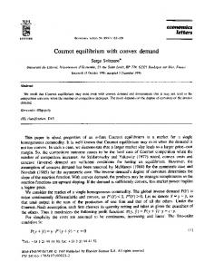
A simple way to understand the problem is by inspection of the firm’s profit as a function of the output of both of them. Fig. 2 shows two surfaces: the gray one is the profit corresponding to f1 , and the black one is the f2 ’s profit function. If the output of f2 is provided (i.e. a fixed value in the f2 ’s output axis), then the decision of f1 is the maximum of the curve resulting from considering f2 ’s output in the gray surface. Since the Nash-equilibrium definition states that both firms’ profit is maximum, we only need to study for each producer the curve built with the maxima of the surface provided the other firm’s output (represented in Fig. 2 with wider lines), i.e. the reaction curves. They are represented in Fig. 3, where it can be observed that the intersection between the two curves is a single point; that is, the Nash equilibrium exists and is unique. Let us turn to study how the algorithm proposed in this paper behaves in the previous two-node case. 4 f1-constrained line assumption f1-constrained line assumption 3.5 (unconstrained) f1-unconstrained line assumption 3 f1-unconstrained line assumption 2.5 (constrained) f2-constrained line assumption 2 f2-constrained line assumption (line unconstrained) 1.5 f2-unconstrained line assumption f2-unconstrained line assumption 1 (line constrained) 0.5 f2’s output

k

f2's output

4.- New sensitivity matrix network state, is computed.

3.5

Fig. 2.- Profit functions of the producers involved in the two-nodes case.

B. Convergence In this section we intend to point out some of the most important features of the algorithm through the investigation of a simple case. We consider a system with two nodes (node 1 and node 2) and a transmission line between the nodes; there are linear demand functions at each of the nodes, and two different generating firms ( f1 and f2 ); all the generation capacity of f1 is located at node 1, and all of the f2 ’s at node 2.

0

1

2

3

4

f1’s output

Fig. 4.- Search mechanism representation of the proposed algorithm

First, a network state is assumed (initially no transmission lines are congested), which allow us to compute the pricesensitivity matrix and solve the quadratic optimization. The reactions curves corresponding to this assumption are represented in Fig. 4, where the solution of the optimization problem (i.e. the Nash-Cournot equilibrium under the assumption that the flow through the line will not be maximum) is the intersection of the curves. The dashed part of each curve represents zones where the assumed line status is not consistent with the decisions of the system operator: for

7

instance, the dashed part of the black curve in Fig. 4 represents a situation where the firm f2 assumes that the line is congested but the corresponding generation forces the line to be uncongested. If both firms assume that the line is to be congested (black and light gray curves) the curves intersect in the dashed region. So, price sensitivity computed as above is not consistent with the initial assumption. Similarly, if both firms assume that the line is to be uncongested, intersection is located again in a dashed region. Therefore, the algorithm converges to a limit cycle and the game’s solution is not found. In order to understand the problem, it is worth noticing that in the full two-stage game (represented in Fig. 2) as described in [5], the producers should solve non-smooth problems which embed the KKT conditions of the system operator, so the best we can expect is a non-smooth stationarity solution. However, our model only studies convex problems and thus we ignore non-smooth points; this can be observed in Fig. 4, where there is an interval of f1 ’s output for which the reaction of f2 is not defined, exactly the points which are maximizers and whose derivatives do not exist. The departure of the proposed model from the Stackelberg approach, although involving a lower amount of computational effort for each player’s optimization problem, implies disregarding these non-smooth points. However, deeper study is needed to examine whether or to what extent this is a shortcoming of our model given the complex nature of the subject: such as the possible existence of a continuum of Nash-Cournot points. Moreover, we are also concerned not just because of convergence problems, but also proper modeling. Anticipating all the network effects sometimes requires not only remarkable analytical capabilities, but perhaps also very precise information on intrinsically uncertain data. VI. CASE STUDY The purpose of this case study is to give an example of the behavior and usefulness of the proposed algorithm, not providing actual policy recommendations or realistic forecasts. So, we consider a European network model that comprises four countries: France, Germany, the Netherlands and Belgium. The Netherlands and Belgium are modeled in further detail, with three nodes (called Krim, Maas and Zwol) and two nodes (Merc and Gram) respectively. Five nodes represent both France and Germany: one represents the aggregated demand (F and D respectively), and four intermediate nodes (no demand or generation). A detailed description of the model can be found at: http://www.electricitymarkets.info/modelcomp/index.html. The eight largest power producers in the four countries are considered: EdF, Electrabel, Essent, RWE, ENBW, Vattenfall, Nuon and E.on Energie. Furthermore, aggregated production of small firms is considered as equivalent competitive generators. Unit characteristics, as well as demand curves at each node and transmission lines characteristics are input data. Table I shows some of these input data. Columns include the

units placed at each node, specifying which firm they belong to, giving the first letters of each name, and their maximum output in megawatts. Table II represents demand data: the first row is the slope of the demand curve in €/MWh per MW, and the second one is its intercept in megawatts. EdF is the nearmonopolist utility in France and, therefore, a regulated one. So, we have decided to consider its market behavior as a nonstrategic agent in all cases. In the model, that means that the 1 T T T EdF S T EdF PEdF is zero in the objective function, term PEdF 2 T since T EdF ST EdF  0 .

TABLE I. GENERATION CAPACITY AND LOCATION Germany France Belgium The Netherlands D F Merc Gram Krim Maas Zwol EON 25669 EdF 85283 El 6635 El 4495 EON 1637 Ess 1410 El 3989 EdF 54 ENB 49 El 116 ENB 8470 Ess 1604 RWE 22886 Nu 2969 Vat 10537 TABLE II. DEMAND DATA D F Merc Gram Krim Maas Zwol Slope 255 225 30 13 26 6 10 Intercept 84139 74163 9769 4159 8625 1856 3154

Three different cases have been studied. The behavior of the remaining firms has been assumed to be different in each of them. The case where firms have the greater foresight ability is studied in case C, and corresponds to the model proposed in this paper. The two first cases are included to show how different assumptions on the behavior of market players can affect the results. In case A all the firms behave as non-strategic agents. In this case, social welfare is maximized, so it can be considered as the benchmark against which market power is to be measured. In case B firms do not consider all the opportunities of exercising market power. Oligopolistic agents decide the production of their units separately (only taking into account the price of the node where each one of their units is located). Therefore, agents consider that output changes in a given bus only affect the price in this same bus. The rationale for this case is that difficulties in forecasting effects of output changes in different parts of the notoriously fragmented European market could lead to this kind of behavior. Mathematically, this is modeled by substituting sensitivity matrix T gT S T g by its diagonal part. The proposed algorithm converges to the nodal prices shown in Table III. Rows represent each of the cases, and columns represent each of the nodes. Nodal prices are given in €/MWh.

A B C

D 24.5 41.8 38.8

TABLE III. NODAL PRICES F Merc Gram Krim 9.4 44.2 30 36.1 9.4 73.9 48.4 60.3 9.4 94.1 87.9 76.3

Maas 33 54.9 71.8

Zwol 31.8 53.3 64.2

The generation of the firms considered is shown in Table IV, in megawatts. Units are represented by two columns:

8

the first of them contains the firm, denoted by the first letters of its name, and the other contains the node where the unit is located. Cases are represented in columns. Numbers in bold type correspond to those units whose generation has reached maximum capacity. TABLE IV. FIRMS GENERATION A B C A 15098 Elec Gram 4242 4215 490 EON D Merc 4992 2934 3880 Krim 1637 Krim 116 116 87 EdF D 54 69310 Zwol 3989 3989 2165 F 23633 Ess Maas 1410 1410 1410 Comp D 6342 Krim 1604 1604 1604 F 18644 8216 9684 RWE D Gram 674 7200 7522 7065 875 ENB D Merc 465 F 49 49 49 Maas 9515 7613 8942 Vat D Krim 518 Nuon Krim 2969 2969 2969 Zwol 3989

B 7522 1637 54 69030 38554 6327 1191 1075 518 518 3989

C 7845 1637 54 69338 38441 6344 1262 1075 518 518 1277

take into account the network-related effects of the production of their units, the power flows distribution represented in Fig. 6 is obtained. Prices in the Benelux countries are higher than in case B. Therefore, there is increased exercise of market power. In order to investigate in detail how can this be done, we will study the results for Electrabel further. Electrabel has units in Belgium (Merc and Gram) and in The Netherlands (Krim and Zwol). Thus, withdrawing power at Gram, Electrabel forces the line Moul-Gram to be constrained, inducing — due to network constraints — a high price at Merc, even with a large production of the units located there. Production of the unit at Merc is higher than in case B, while Electrabel is using the production of the unit at Gram to increase the price of Merc. Zwol Krim

Diel Maas

Merc

Rom

A. Competitive Prices and productions are collated in Table III and Table IV. Observe that in the perfect competition case (A), prices are much lower than in the other two cases. The power flow for this case is shown in Fig. 5. Arrows between nodes represent transmission lines, and the direction of the power flow through them. Wide arrows represent constrained lines. Zwol Krim

Diel Maas

Merc Rom Ucht

Lonn

F

D

Gram

Avel

Moul

D

Gram

Avel

Ucht

Lonn Moul

F

Eich Muhl

Fig. 6. Network state in case C

On the other hand, the price in Germany is lower than in case B. Moreover, production of all of the strategic agents located there is higher. Note that this is true also for Vattenfall, that has no generation outside Germany. The main reason is that sensitivity matrix S has changed from case A to B, because of the different network state: in case B the elasticity in Germany (38.57 €/MWh per MW) is lower than that of case C (28.44 €/MWh per MW), so market power in Germany is higher in case B.

Eich Muhl

Fig. 5. Network state in cases A and B

B. Incomplete price response case The main effect of the higher market power is that prices at every node, but France, are higher than in the competitive case. The price of France should not change too much (and in practice does not), because EdF is almost the only firm producing at France (ENBW unit has only 49 MW capacity), and it is competitive. Table IV shows that strategic firms in Germany withdraw power, so there is a higher price there. However, physical output in the Netherlands is the maximum in case B, the same as in case A. Considering that the price sensitivities are the same as in case A although they were not considered (since the network state has not changed) it can be concluded that firms in the Netherlands obtain more profit due to the high price induced by the network than the situation that would be obtained by withdrawing power. This highlights that, when the network is considered, a firm located at a certain node is not always interested in exercising market power. C. Strategic case When firms are considered as strategic agents, and they

VII. CONCLUSIONS A new algorithm to compute Nash-Cournot equilibria in power networks has been introduced, capable of representing the fact that market players can anticipate how the production of one of their units will affect the whole network. In addition, the algorithm has been tested in a stylized European power system, showing how the results of the model change when the rational behavior of firms is considered. We conclude that market price in a bus is not only dependent on the competitiveness of that bus (as measured by price elasticity) but also on power flows on the whole network. Currently, consideration of network congestions modify the demand faced by the firms located at a certain node, and therefore modify the price elasticity of that node. Consequently, depending on the case, competition may be decreased or increased by the interconnection with a number of non-obvious effects, as shown in the sample cases. Our model represents a tool to simulate these types of complex network effects in meshed electricity markets, with reasonably low computational effort; they may be useful in analyzing the behavior of oligopolistic firms in wide-area markets. We believe that it can be advantageously used both for regulatory purposes and for

9

strategic analysis carried out by market participants.

It is easy to check C  

ACKNOWLEDGEMENTS We would like to thank the Energy Research Centre of the Netherlands, and especially F. A. M. Riekers, for providing the test data set. We also would like to thank K. Neuhoff, A. Ehrenmann, M. G. Boots, B. F. Hobbs, F. A. M. Riekers and C. Vázquez for their valuable comments. The French, Dutch and Belgium regulators funded the workshops where the study herein reported took shape. The comments of three anonymous referees and of the editor are also acknowledged.

B  S D    πzT  (4)      C     B T  where new matrices B and C are defined. Matrix C is singular. So, let us consider regular matrix C    C   I , with  some small number, and the matrix

S D   the solution of (4) when C is substituted by C   . A related equation is B  S 0    πzT   A  T  D   C      0   B An important property, used in the sequel, is that The reason can be gathered from (3).

Each column of S D0  0 can be computed by solving (3) with

 P  0 . Now, if there are no changes in the injected power, there are not going to be changes in the demanded powers either (as they are perturbations on the optimum), i.e.:  D  0 . So, it can be written that B  S    S 0    0   A D  T  D  T B C       B   Therefore, for   0 1

BT

 S

D

  A  I 

   S D0     BC  1 B T . So 1

S D    S D0    A  BC   B T



 1   BC   B T 



1

1

A





1

1 

1

BC   B T 



1

T  BC   B 



1

A

So A S D    S D0   is symmetric. By taking limits





lim 0 A S D    S D0    lim 0 A S D    S

APPENDIX B: MATRIX S IS POSITIVE Let us partition C   as

 I C      Cr

F CrT    , Cr   0  I   0

I E M

   

1

0



2



I  Cr CrT

  1   

So

  2 I

1

BC   B T   0 I

 CrCrT



1 

0 I   

Cr CrT , is a symmetrical non-negative matrix (because for 2

x , xT CrCrT x  CrT x  0 ). Then, there are two

every

   K 

 A  T  B

A  BC  



 fulfills k   C C   K .So      I  C C      k   

must be real)  Cr CrT

Let us write (2) as

   0 .



 2 T CrT    I  Cr Cr   I   0 

 I   Cr

constants k , K  0 such that every Cr CrT eigenvalue (that

APPENDIX A: MATRIX S IS SYMMETRIC

lim 0 S D0

1

1 

 

1

1

2

Therefore



 2 K

T r r

T 1 r r

2



2



1

1

1   BC   B T     2  k  



.

1

and



 2 K



1

 max i  

1

  BC   B T  A 



1 

2      k



1

 min i 

So



 2    K 



1

  max i   



1







  A S D    S D0       2  k   As then



 lim 0   2  K 







1



1

  max i   

  min i    1

1

 max i 

1

0



1  S   lim 0  A S D    S D0     min i   0

 which proves the claim.

REFERENCES [1] Neuhoff, K., J. Barquín, M. G. Boots, A. Ehrenmann, B. F. Hobbs, F. A. M. Rijkers, M. Vázquez, "Network-constrained Cournot models of liberalized electricity markets: the devil is in the details". Energy Economics. 27: p. 495-525 2005. [2] Barquín, J., E. Centeno, J. Reneses, "Medium term generation programming in competitive environments: a new optimization approach for market equilibrium computing". IEE Proceedings Generation, Transmission and Distribution. 151(1): p. 119-126 2004. [3] Ehrenmann, A., "Manifolds of multi.leader Cournot equlibria". Operations Research Letters. 32(2): p. 121-125 2004. [4] Hobbs, B. F., F. A. M. Rijkers, "Strategic generation with conjectured transmission price responses in a mixed transmission pricing system I: formulation and II: application". IEEE Transactions on Power Systems. 19(2): p. 707-717, 872-879 2004. [5] Ehrenmann, A., K. Neuhoff, "A comparison of electricity market designs in networks". CMI Working Paper 31. 2003. [6] Metzler, C., B. F. Hobbs, J. S. Pang, "Nash-Cournot equilibria in power markets on a linearized DC network with arbitrage: formulations and properties". Networks and Spatial Economics. 3(2): p. 123-150 2003. [7] Neuhoff, K., "Combining energy and transmission market mitigates

10

[8]

[9]

[10]

[11]

[12]

[13]

[14] [15]

market power". CMI Working Paper, Dept. of Applied Economics, Cambridge University. 2003. Day, C. J., B. F. Hobbs, J.-S. Pang, "Oligopolistic competition in power networks: a conjectured supply function approach". IEEE Transactions on Power Systems. 17(3): p. 597-607 2002. Daxhelet, O., Y. Smeers, "Variational inequality models of restructured electric systems", in Applications and Algorithms of Complemetarity, M.C. Ferris, O.L. Mangasarian, and J.-S. Pang. 2001, Kluwer: Dordrecht. Ventosa, M., M. Rivier, A. Ramos, A. García-Alcalde. "An MCP approach for hydrothermal coordination in deregulated power markets", in IEEE/PES summer meeting. Seattle, Washington, USA. 2000 Yuan, W. J.-. Y. Smeers, "Spatial oligopolistic electricity models with Cournot generators and regulated transmission prices". Operations Research. 47(1): p. 102-112 1999. Cardell, J., C. C. Hitt, W. W. Hogan, "Market power and strategic interaction in electricity networks". Resource and Energy Economics. 19(1-2): p. 109-137 1997. Scott, T. J., E. G. Read, "Modeling hydro reservoir operation in a deregulated electricity market". International Transactions in Operational Research. 3: p. 243-253 1996. Schweppe, F. C., M. C. Caramanis, R. E. Tabors, R. E. Bohn, "Spot pricing of electricity". Kluwer Academic Publishers. 1988. Hashimoto, H., "A spatial Nash equilibrium model", in Spatial price equilibrium: Advances in theory, computation and application, P. Harker. 1985, Springer-Verlag: Berlin. p. 20-40.

BIOGRAPHIES Julián Barquín (M' 94) took an Industrial Engineering degree and an Industrial Engineering Doctorate from Universidad Pontificia Comillas, Madrid, in 1988 and 1993 respectively; he graduated in Physical Sciences in 1994. He belongs to the research staff at the Technological Research Institute [Instituto de Investigación Tecnológica, IIT]. His present interests include control, operation and planning of power systems. Miguel Vázquez took an Industrial Engineering degree from Universidad Politécnica de Madrid in 2004. He is currently a research assistant at the Technological Research Institute [Instituto de Investigación Tecnológica, IIT]. He is interested in power systems and markets.