Covariance Descriptors for 3D Shape Matching and Retrieval - Hal

Covariance Descriptors for 3D Shape Matching and Retrieval Hedi Tabia, Hamid Laga, David Picard, Philippe-Henri Gosselin

To cite this version: Hedi Tabia, Hamid Laga, David Picard, Philippe-Henri Gosselin. Covariance Descriptors for 3D Shape Matching and Retrieval. IEEE Conference on Computer Vsion and Pattern Recognition, Jun 2014, Columbus, Ohio, United States. 8 p., 2014.

HAL Id: hal-01022970 https://hal.archives-ouvertes.fr/hal-01022970 Submitted on 11 Jul 2014

HAL is a multi-disciplinary open access archive for the deposit and dissemination of scientific research documents, whether they are published or not. The documents may come from teaching and research institutions in France or abroad, or from public or private research centers.

L’archive ouverte pluridisciplinaire HAL, est destin´ee au d´epˆot et `a la diffusion de documents scientifiques de niveau recherche, publi´es ou non, ´emanant des ´etablissements d’enseignement et de recherche fran¸cais ou ´etrangers, des laboratoires publics ou priv´es.

Covariance Descriptors for 3D Shape Matching and Retrieval Hedi Tabia1 Hamid Laga2,3 David Picard1 Philippe-Henri Gosselin1,4 1 ETIS/ENSEA, University of Cergy-Pontoise, CNRS, UMR 8051, France 2 Phenomics and Bioinformatics Research Centre, University of South Australia 3 Australian Centre of Plant Functional Genomics 4 INRIA Rennes Bretagne Atlantique, France

Abstract

sis settings, many authors attempted to adapt popular local image descriptors to 3D shapes. Examples include the 3D SIFT [41] and the 3D Shape Context [11, 17]. One of the main strengths of local features is their flexibility in terms of type of analysis that can be performed with. For instance they can be used as local descriptors for shape matching and registration but can be also aggregated over the entire shape, using the Bag of geometric Words (BoW), to form global descriptors for recognition, classification and retrieval [5]. These techniques, however, face two main concerns. First, local features do not capture the spatial properties or structural relations between shape elements. Second, often 3D shape collections exhibit large inter-class and intra-class variability that cannot be captured with a single feature type. This triggers the need for combining different modalities or feature types. However, different shape features have different dimension and scale, which makes their aggregation difficult without normalizing or using blending weights. To overcome some of these shortcomings, Behmo et al. [2] proposed to compute a graph based representation that captures the spatial relations between features. Bronstein et al. [5] extended this approach and proposed spatially-sensitive bags of features by considering pairs of geometric words. Laga et al. [18] combined both geometric and structural features to capture the semantics of 3D shapes. While these representations take into account the spatial relations between features of the same type, they are limited when it comes to handling multimodal features. Recently, the image analysis community showed a growing interest in characterizing image patches with the covariance matrix of local descriptors rather than the descriptors themselves. They have been used for object detection and tracking [29, 38, 39, 21], texture classification [38], action recognition and face recognition [13]. The use of covariance matrices has several advantages. First, they provide a natural way for fusing multi-modal features without normalizing. Second, covariance matrices extracted from different regions have the same size. This enables comparing any regions without being restricted to a constant window

Several descriptors have been proposed in the past for 3D shape analysis, yet none of them achieves best performance on all shape classes. In this paper we propose a novel method for 3D shape analysis using the covariance matrices of the descriptors rather than the descriptors themselves. Covariance matrices enable efficient fusion of different types of features and modalities. They capture, using the same representation, not only the geometric and the spatial properties of a shape region but also the correlation of these properties within the region. Covariance matrices, however, lie on the manifold of Symmetric Positive Definite (SPD) tensors, a special type of Riemannian manifolds, which makes comparison and clustering of such matrices challenging. In this paper we study covariance matrices in their native space and make use of geodesic distances on the manifold as a dissimilarity measure. We demonstrate the performance of this metric on 3D face matching and recognition tasks. We then generalize the Bag of Features paradigm, originally designed in Euclidean spaces, to the Riemannian manifold of SPD matrices. We propose a new clustering procedure that takes into account the geometry of the Riemannian manifold. We evaluate the performance of the proposed Bag of Covariance Matrices framework on 3D shape matching and retrieval applications and demonstrate its superiority compared to descriptor-based techniques.

1. Introduction Quantifying shape similarity between 3D objects, hereinafter refereed to as shape analysis, is central to many computer vision and pattern recognition tasks. The common factor in existing techniques is the use of shape signatures that capture the main properties of 3D objects. While early methods focused on global descriptors that are invariant under rigid transformations [19], the use of local features has gained a significant momentum in the past few years [5, 37, 33]. Due to their good performance in many image analy1

size or specific feature dimension. Covariance matrices, however, lie on the manifold of Symmetric Positive Definite (SPD) tensors (Sym+ d ), a special type of Riemannian manifolds. This makes the development of classification and clustering methods on the space of SPD matrices quite challenging. Many authors attempted to generalize computational methods, originally designed for Euclidean spaces, to Riemannina manifolds. Jayasumana et al. [14], for example, generalized the powerful kernel methods to manifold-valued data, such as covariance matrices, and has demonstrated their usage in pedestrian detection, visual object categorization, texture recognition and image segmentation. Similarly, Faraki et al. [9] demonstrated the usage of bag of covariance matrices in the classification of human epithelial cells in 2D images. In this paper, we generalize the ideas presented in [29, 38] to 3D shape analysis problems, particularly to 3D shape matching and recognition and to 3D shape retrieval. Our idea is to represent a 3D model with a set of n landmarks sampled (uniformly or randomly) on its surface. Each landmark has a region of influence, which we characterize with the covariance of features of different types. Each type of features captures some properties of the local geometry. Covariance matrices are not elements of the Euclidean space, they are elements of the Lie group, which has a Riemannian structure. Therefore, matching with covariance matrices requires the computation of geodesic distances on the manifold using a proper metric. We show how such dissimilarity measure can be computed in an efficient way and demonstrate its performance in 3D face matching and recognition. We also propose an extension of the BoW approach to nonlinear Riemannian manifolds of covariance matrices. Our dictionary construction procedure uses geodesic distances and thus it captures effectively the structure of the manifold. We demonstrate the performance of the proposed framework in several 3D shape analysis applications. We show that covariance descriptors perform better than individual features on 3D correspondence and registration tasks and on 3D face matching and recognition. We also evaluate the retrieval and classification performance of the Bag of Covariance matrices on 3D shape retrieval and recognition using standard benchmarks. Our contributions are three-fold. First, we propose covariance matrices as new descriptors for 3D shape analysis. While similar descriptors have been proposed for object tracking and texture analysis in 2D, it is the first time that covariance based analysis is explored for 3D shape analysis. Second, the framework enables the fusion of multiple and heterogeneous features without the need for normalization. Finally, using a Riemannian metric on the manifold of covariance matrices, we introduce the concept of Bag of Covariance matrices for 3D shape classification and retrieval. The rest of the paper is organized as follows. We intro-

duce covariance matrices for 3D shape analysis in Section 2 and review the basic concepts of Riemannian geometry in Section 3. Section 4 presents how covariance matrices can be used in comparing 3D models. Section 5 extends the Bag of Features paradigm to the non-linear space of covariance matrices of 3D shapes. We evaluate our approach on various datasets in Section 6 and conclude in Section 7.

2. Covariance matrices on 3D shapes We represent a 3D shape as a set of overlapping patches {Pi , i = 1 . . . m}, each patch Pi is extracted around a representative point pi = (xi , yi , zi )t . For each point pj = (xj , yj , zj )t , j = 1 . . . , ni , in the patch Pi , we compute a feature vector fj , of dimension d, that encodes the local geometric and spatial properties of the patch. The following properties can be used: • F1: The location ofP the point pj with respect to the ni pk . It is given by pj − pc . patch center pc = n1i k=1 • F2: The distance of the point pj to pi .

• F3: The volume of the parallelepiped formed by the coordinates of the point pj . Note that our framework is generic and thus other features can also be added to the representation. Examples include the norm of the gradient, the two principal curvatures k1 and k2 , the mean and Gaussian curvatures, the shape p index [16], the curvedness at pi , which is defined as (k12 + k22 )/2, the shape diameter function [12, 30], and the scale-invariant heat kernel signature [6]. Let {fj }j=1..n be the d-dimensional feature vectors computed over all points inside Pi . We represent a given 3D patch Pi with a d × d covariance matrix Xi : n

Xi =

1X T (fj − µ) (fj − µ) n j=1

(1)

where µ is the mean of the feature vectors computed in the patch Pi . The covariance matrix Xi is a symmetric matrix. Its diagonal elements represent the variance of each feature and its off-diagonal elements represent their respective correlations. It has a fixed dimension (d × d) independently of the size of the patch Pi .

3. Riemannian geometry of SPD matrices For the sake of completeness, we present here the mathematical properties of the space of covariance matrices and the metrics that have been proposed for comparing them.

3.1. The space of covariance matrices Let M = Sym+ d be the space of all d × d symmetric positive definite matrices and thus non-singular covariance matrices. Sym+ d is a non-linear Riemannian manifold, i.e. a differentiable manifold in which each tangent space TX at

X has an inner product h·, ·iX∈M that smoothly varies from point to point. The inner product induces a norm for the tan2 gent vectors y ∈ TX such that kyk = hy, yiX . The shortest curve connecting two points X and Y on the manifold is called a geodesic. The length d(X, Y ) of the geodesic between X and Y is a proper metric that measures the dissimilarity between the covariance matrices X and Y . Let y ∈ TX and X ∈ M. There exists a unique geodesic starting at X and shooting in the direction of the tangent vector y. The exponential map expX : TX 7→ M maps elements y on the tangent space TX to points Y on the manifold M. The length of the geodesic connecting X to Y is given by d(X, expX (y)) = kykX . Machine learning algorithms require the definition of metrics for comparing data points. When data lie in the Euclidean space, Euclidean distance is often used as the natural choice of metric. Covariance matrices, however, lie on a non-linear manifold and thus, efficient algorithms are required for computing geodesics and their lengths. Geodesic lengths can then be used as a metric for subsequent machine learning algorithms. In this paper, we focus on the computation of geodesic lengths. Most of the existing classifiers (e.g. the nearest neighbor classifier) only requires a notion of distance between points on the manifold M. We use the distance proposed in [28] to measure the dissimilarity of two covariance matrices.

3.2. Geodesic distance between covariance matrices

The geodesic distance between two points on Sym+ d is then given by: d2g (X, Y )

= =

hlogX (Y ) , logX (Y )iX    1 1 trace log2 X − 2 Y X − 2

(2)

An equivalent form of the affine-invariant distance metric has been given in [10] and [25] in terms of joint eigenvalues of X and Y . We will use this metric to derive algorithms for 3D shape analysis using covariance matrices as local descriptors.

4. 3D shape matching using SPD matrices In this section, we propose a metric for matching 3D shapes using covariance matrices as descriptors and the Riemannian metric as a measure of dissimilarity. Let us consider a point pi represented by the covariance descriptor Xi on the first 3D model and a point qj represented by the covariance descriptor Yj on the second 3D model. Let c (pi , qj ) = dg (Xi , Yj ) denote the cost of matching these two points. It is defined as the geodesic distance on the Riemannian manifold between the two descriptors Xi and Yj . Given the set of costs cij between all pairs of points pi on the first 3D shape and qj on the second 3D shape, we define the total cost of matching the two 3D shapes as: X
c pi , qϕ(i) C(ϕ) = (3) i

The Riemannian metric of the tangent space TX ata  1 − 12 point X is given as hy, ziX = trace X yX −1 zX − 2 . The exponential map associated to the met Riemannian  1 1 − 21 − 12 2 2 ric expX (y) = X exp X yX X is a global diffeomorphism (a one-to-one, onto, and continuously differentiable mapping in both directions). Thus, its inverse is uniquely defined at everypoint on the manifold:  1 1 1 1 − logX (Y ) = X 2 log X 2 Y X − 2 X 2 . The symbols exp and log are the ordinary matrix exponential and logarithm operators, while expX and logX are manifold-specific operators, which depend on the point X ∈ Sym+ d . The tangent space of Sym+ d is the space of d×d symmetric matrices and both the manifold and the tangent spaces are of dimension m = d(d + 1)/2. For symmetric matrices, the ordinary matrix exponential and logarithm operators can be computed in the following way. Let X = U DU T be the eigenvalue decomposition of the symmetric matrix X. The exponential seP∞ k ries is defined as: exp (X) = k=0 Xk! = U exp (D) U T , where exp (D) is the diagonal matrix of the eigenvalue exponentials. Similarly, the logarithm is given by log (X) = P∞ −1k−1 k (X − I) = U log (D) U T . The exponential k=1 k operator is always defined, whereas the logarithms only exist for symmetric matrices with strictly positive eigenvalues.

Minimizing C(ϕ), subject to the constraint that the matching is one-to-one, gives the best permutation ϕ(i). This is an assignment problem, which can be solved using the Hungarian method. In our implementation, we use the shortest augmenting path algorithm [15]. The input to the assignment problem is a square cost matrix with entries cij . The result is a permutation ϕ(i) such that Equation 3 is minimized. The minimum of this cost function is then used as the dissimilarity between the two 3D models.

5. Bag of Words on Riemannian manifold We extend the Bag of Words (BoW) approach [32, 24] to covariance matrices for 3D shape analysis. In the classical BoW approach, a 3D model is represented as a collection of local descriptor prototypes, called visual words, given a well chosen vocabulary, i.e. the codebook. BoW representations have been widely adopted by the 3D shape analysis community [37, 5]. One of their advantages in 3D shape retrieval is their ability to aggregate a large number of local descriptors into a finite, low dimensional, histogram. The dissimilarity between a pair of 3D models becomes then a distance between their respective histograms, which is computationally more efficient than minimizing a cost function. The first step of the BoW approach consists of approximating a set of training samples with a finite set of visual

words, the centers, which form the codebook. The codebook is often obtained using clustering algorithms, such as k-means. A good codebook should represent the original data with minimum distortion. The distortion is usually defined as the average mean square distance of all the training P 1 2 ˆ points to the centers: M SD = |S| X∈S dg (X, X) where the set S denotes the input data set, |S| its cardinality, and ˆ is the center of the cluster to which X is assigned. The X classification of a query model involves the assignment of the descriptors computed on the model into one of the codebook elements. This process involves the computation of distances between feature points. When these points lie in Euclidean spaces, the computation of Euclidean distances in straightforward. In what follows, we describe how to extend this concept to covariance matrices, which are elements of the non-linear Riemannian manifold Sym+ d and thus require efficient algorithms for computing geodesic distances.

5.1. Center computing Let S = {Xi }i=1..N be a set of points on M = Sym+ d. The intrinsic mean of points in Riemannian manifold is the point on Sym+ d that minimizes the sum of squared geodesic distances: ˆ = arg min X

X∈M

N X

d2g (Xi , X) ,

(4)

i=1

where dg is the geodesic distance between two points on the manifold.PThe mean is the solution to the nonlinear matrix N equation i=1 logX (Xi ) = 0, which can be solved using a gradient descent procedure. At each iteration, the estimate of the mean is updated as follows: # " N X 1 t+1 ˆ logXˆ t (Xi ) . (5) X = expXˆ t N i=1 Equation 5 starts by mapping the points onto the tangent space to the manifold at the current estimate of the mean (using inverse exponential map), computes an estimate of the mean in the tangent space, and maps back the estimated mean onto the manifold using exponential map. This process is iterated until convergence. The iterative use of the logarithmic and exponential maps makes this method computationally expensive. To overcome this, many solutions can be used: • One can use the k-medoid algorithm instead of kmeans. When computing the codebook, k-means tries to find the true mean of the data. Thus, the minimization in Equation 4 is over the entire manifold. Kmedoids on the other hand constrains the center to be one of the data points and thus the search space for the best solution is significantly reduced. Using K-medoid requires the computation of the pairwise distances between all training data, which can be time consuming.

• Alternatively, one can map all the training points to the tangent space of the manifold at one point (e.g. mean point), obtaining an Euclidean representation of the manifold-valued data. As stated in [14], this mapping does not globally preserve distances, resulting in a poor representation of the original data distribution. • The third solution is to use the geodesic distance dg with the Frobenius distance when computing the centers of k-means. The idea is that the Euclidean average of covariance matrices lies in the Riemannian manifold, as stated in [4]. Indeed, any non-negative linear combination of symmetric positive definite (SPD) matrices is an SPD matrix. This implies that the linear avˆ of X1 , ..., XN given by: X ˆ = 1 (X1 + ... + erage X N XN ) is an SPD matrix, hence belongs to the Riemannian manifold. The Frobenius distance from which the linear average came is given by: 2 X d2F ro (X1 , X2 ) = (6) (X1 − X2 )ij . 1≤i,j≤n

We tested those three codebook constructions and studied the repartition of the final set of centers obtained from each solution in the space of Hermitian forms, SPD matrices.

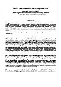
5.2. Center repartitions After running the three earlier mentioned solutions, we evaluate the distance between each center and the identity element In of this space. This distance is computed according to Equation 2 when the geodesic metric is used, and Equation 6 when the Frobenius metric is chosen. Figure 1 shows the repartition of the centers after running k-means on a sample of 104 Hermitian forms, using three variants based on geodesic distance (presented in the previous section), and a fourth variant based on the Frobenius distance (cf. Eq. 6). In each sub figure, the origin represents the identity matrix In and a green symbol represents ˆ i placed on a circle of radius equal to its distance a center X   ˆ i ) = 2π Pcard(Xˆ i ) from the identity. The angles, α(X ˆ k card(Xk ) n o ˆk (where X are the centers), that surround the dif1≤k≤K

ferent centers are proportional to the size of their corresponding cluster. From Figure 1-(a) and (c), one can notice that the size of different classes is almost equal. This demonstrates that the data points are equally partitioned when using the geodesic distance. On the other hand, Figure 1-(b) and (d) show that large classes contain most of the data samples. This shows that the use of Frobenius distance when assigning the points to their closest centers is not suitable for covariance matrices. It also shows that approximation using the tangent space of the mean data point voids one of the benefits of using the geodesic distance.

90

90 1 120

60

150

30

0

330

210

300

30 0.4

0.4

0.2

0.2

180

0

330

210

300

240

150

30

0.4

0.2

180

0.6

0.6

150

30 0.4

0.2

60 0.8

0.8

0.6

150

120

60

0.8

0.6

1

1 120

60

0.8

240

90

90

1 120

180

0

330

210

300

240

180

0

330

210

240

300

270

270

270

270

(a)

(b)

(c)

(d)

Figure 1. (a) k-medoid using geodesic distance, (b) k-means on the tangent space of the mean data point (c) k-means using Geodesic distance and linear update of centers and (d) k-means using Frobenius distance, K = 20 classes.

Algorithm 1 Codebook construction Require: n o N data points to classify and an initial set of K data points ˆk chosen randomly. X k=1..K

Ensure: labeled data points and K centers iter = 1; M SEiter = 0; M SEiter−1 = 1; while (iter ≤ maxIter) && (M SEiter 6= M SEiter−1 ) do M SEiter = 0 for i = 1 to N do d = M AXV AL for k = 1 to K do ˆ iter , Xi ) using eq. 2 d k = d g (X k if d > dk then d = dk kmin = k end if end for ˆ iter Assign Xi to the center X kmin M SEiter + = dkmin end for for k = 1 to K do P ˆ iter+1 = 1 X i (Xik ) k Nk end for iter + + end while

Another observation that can be made from Figures 1(a), (b) and (c) is that the centers are located at different distance levels from the identity matrix. This demonstrates that the geodesic distance is more discriminant for covariance matrices than the Frobenius one as shown in Figure 1(d). We can conclude that the geodesic distance gives better repartition of the data samples than the Frobenius distance. We can also see that the K-medoid algorithm (Figure 1-(a)) behaves better than the other solutions. However, as mentioned earlier, using the K-medoid algorithm, all pairwise distances between training data have to be computed, which is time consuming when dealing with large data samples. The third solution (see Figure 1-(c)) behaves similarly to Kmedoid solution. In this paper, we used the third solution, which is detailed in Algorithm 1 for codebook construction.

5.3. Signature computing We describe 3D shapes using vectors of visual word frequencies. For a given 3D model, each point Pi represented

by its covariance descriptor is assigned to its closest center using the geodesic distance of Equation 2. The frequency of a visual word in a given shape is simply the number of times a given visual word appears in that model. For best performance, we perform a normalization step of the signature. In our experiment, we use the 0.3 power norm. At the retrieval stage, 3D shapes are ranked using as metric the cosine of the angle between the query vector and all shape vectors in the database.

6. Experimental results We carried out an extensive set of experiments to evaluate and verify the effectiveness of the proposed method in matching and retrieving 3D models.

6.1. 3D face matching and recognition We analyzed the performance of the proposed covariance descriptors on 3D face recognition tasks. We used the GavabDB1 dataset, which is among the most noise-prone datasets currently available in public domains. It contains 549 three-dimensional facial surfaces of 61 different individuals (45 males and 16 females). Each individual has nine facial surfaces with two frontal views at neutral expression, two views rotated with +35 degrees around the x-axis, one looking up and another looking down, both in neutral expression, two profile views (left and right), both in neutral expression, and three frontal images with facial expressions (laugh, smile and a random expression chosen by the user). Thus, the database provides large variations with respect to pose and to facial expressions. All the individuals are Caucasian and their age varies between 18 and 40 years old. We have first preprocessed the surfaces to remove spikes, fill in the holes and align them. We have then uniformly sampled m = 100 feature points on the 3D face scan. To ensure a uniform sampling, we first select a random set of vertices on the face and then apply few iterations of Lloyd relaxation algorithm. We then generate a set of patches {Pi , i = 1 . . . m}, each patch Pi has a radius r = 10% of 1 http://www.gavab.es/recursos

en.html

Methods

Neutral

Expression

Proposed method 100% 93.30% Drira et al. [8] 100% 94.54% Li et al. [40] 96.67% 93.33% Mahoor et al. [22] 95.00% 72.00% Moreno et al. [26] 90.16% 77.90% Table 1. Results on Gavab dataset.

Overall

Methods

2-Tier

DCG

94.91% 94.67% 94.68% 78.00% NA

Covariance Method 0.977 0.732 0.818 Graph-based [1] 0.976 0.741 0.911 PCA-based VLAT [35] 0.969 0.658 0.781 Hybrid BoW [20] 0.957 0.635 0.790 Hybrid 2D/3D [27] 0.925 0.557 0.698 Table 2. Results on McGill dataset.

0.937 0.933 0.894 0.886 0.850

the radius of the shape’s bounding sphere, and it is identified with its corresponding seed point pi . For each patch we compute a 5 × 5 covariance matrix that encodes the features F1, F2 and F3 defined in Section 2. We then use the matching method presented in Section 4 to compare 3D faces. In this experiment, the first frontal facial scan of each subject was used as gallery while the others were treated as probes. To objectively evaluate our method for face recognition, we present results in the form of recognition rate, see Table 1. We can see that our method achieves a recognition rate of 100% on the faces of neutral expressions. This performance is similar to the approach of Drira et al. [8]. Our approach performs slightly lower than the approach of Drira et al. on faces with expressions (93.3% vs. 94.54%). It is interesting to note that in [8], authors manually landmarked points on all the face scans in the dataset to ensure an efficient face registration. Table 1 also shows that the proposed method outperforms all the other methods and achieves the best overall result when the neutral and expressive faces are merged together.

6.2. 3D shape retrieval We have analyzed the performance of the proposed covariance-based descriptors on 3D shape retrieval tasks using three different databases: • The McGill2 database [31], which contains 255 objects divided into ten classes. Each class contains one 3D shape under a variety of poses. • The SHREC07 dataset3 for global 3D shape retrieval. It contains 400 models evenly distributed into 20 shape classes. The experiment was designed so that each model was used in turn as a query against the remaining elements of the database, for a total of 400 queries. • The SHREC07 dataset4 for partial 3D shape retrieval. It contains a database of 400 models and a query set of 30 composite models. The dataset exhibits diverse variations including pose change, shape variability, and topological variations (note that four of the 20 classes contain non-zero genus surfaces) [23]. 2 http://www.cim.mcgill.ca/

shape/benchMark/

3 http://watertight.ge.imati.cnr.it/ 4 http://partial.ge.imati.cnr.it/

NN

1-Tier

We randomly sample m = 600 points on the 3D mesh. We assign for each point pi a patch Pi , i = 1 . . . m, on which we compute a covariance descriptor. We extract the local patch Pi by considering the connected set of facets belonging to a sphere centered at pi and of radius r = 15% of the radius of the shape’s bounding sphere. We then compute a 5 × 5 covariance matrix from the features F1, F2 and F3 defined in Section 2. We then use our Riemannian BoW method (Section 5) to compare 3D shapes. We use a codebook of size 250 visual words. We have evaluated the proposed method using various performance measures, namely: Precision-Recall graphs, Nearest Neighbor (NN), the First Tier (1-Tier), The Second Tier (2-Tier), and the Discounted Cumulative Gain (DGC). 6.2.1

Watertight 3D shape retrieval

Table 2 summarizes the retrieval performance of the proposed method on the McGill dataset. We compare our results to various state-of-the-art methods: the Hybrid BoW [20], the PCA-based VLAT approach [35], the graphbased approach of Agathos et al. [1], and the hybrid 2D/3D approach of Papadakis et al. [27]. Although the proposed method does not consider structural information of shapes, it achieves the best performance on NN and DCG. The graph-based algorithm performs slightly better than ours on 1-Tier and 2-Tier. The robustness of the Riemannian BoW method to nonrigid deformations of shapes is probably due to the local descriptors we used in building the covariance matrices. 6.2.2

Global shape retrieval

We used the SHREC07 dataset to evaluate the performance of our method in global shape retrieval tasks. Figure 2 summarizes and compares the precision-recall performance of our approach against three state of the art methods: the Hybrid BoW of Lavou´e [20], the curve based method of Tabia et al. [34] and the BoW method of Toldo et al. [37]. We can clearly see that covariance-based BoW achieves significantly better precision than previous methods for low recall values. The precision is kept over 70% when half of the relevant objects have been returned (recall equals to 0.5). Since low recall values correspond to the first objects retrieved, this result shows that our method is significantly

1

Methods

NN

1-Tier

2-Tier

DCG 0.9

Covariance Method 0.930 0.623 0.737 0.864 Hybrid BoW [20] 0.918 0.590 0.734 0.841 Tabia et al. [34] 0.853 0.527 0.639 0.719 Table 3. Results on SHREC07 for global 3D shape retrieval.

0.8

0.7

0.6

0.5 1

0.4

0.9

Proposed met hod

0.8

Lavoue 2012

0.3

T abia et al. 2011

Precision

0.7

T oldo et al. 2009

0.2

T ierny et al. 2009

0.6

ERG

0.1 0.5

CORNEA

0.4

Proposed met hod

0.3

T oldo et al. 2009

0 0

Lavoue 2012

50

100

150

200

250

300

350

Figure 4. NDCG curves of our method compared to recent state of the art methods, for the SHREC 2007 Partial retrieval dataset.

T abia et al. 2011 0.2 0.1 0

0

0.1

0.2

0.3

0.4

0.5

0.6

0.7

0.8

0.9

1

Recall

Figure 2. Precision vs recall curves of our method compared to recent state of the art method [34], for the SHREC 2007 global shape retrieval dataset.

Figure 3. Some examples of query objects (the most-left object in each row) from the SHREC07 Partial retrieval dataset and the top-6 retrieved models.

better than the other methods in retrieving relevant models at the top of the ranked list of results. Table 3 also shows that the proposed approach outperforms the state-of-the-art on NN, 1-Tier, 2-Tier and DCG measures. 6.2.3

Partial shape retrieval

Partial shape similarity is a complex problem, which has not been fully explored in the literature. We have tested the performance of the proposed method on this problem using the SHREC07 partial retrieval dataset. Figure 3 shows some query models and the top-6 results returned by our method. We can observe that all the retrieved models are highly relevant to the queries. We conducted a quantitative evaluation using the Normalized Discounted Cumulated Gain vector (NDCG) [23]. For a given query, NDCG[i] represents the relevance to the query of the top-i results. It is recursively defined as DCG [i] = G [i] if i = 1 and DCG [i] = DCG [i − 1] +

G [i] × log(i) otherwise where G [i] is a gain value depending on the relevance of the ith retrieved model (2 for highly relevant, 1 for marginally relevant and 0 otherwise). The NDCG is then obtained by dividing the DCG by the ideal cumulated gain vector. Figure 4 shows the NDCG curves of the proposed method and six other state-of-the-art methods: the Hybrid BoW [20], the curve-base method [34], the BoW method of Toldo et al. [37], the graph-based technique of Tierny et al. [36], the extended Reeb graphs (ERG) [3] and the curveskeleton based many-to-many matching (CORNEA) [7]. We can clearly see that our method outperforms them. The high performance of the proposed method is due to the descriptive power of the covariance descriptor that efficiently discriminates relevant regions of each model. Discussion. Analyzing shapes with covariance matrices has several advantages compared to individual descriptors: (1) covariance matrices enable the fusion of multiple heterogeneous features of arbitrary dimension without normalization or blending weights, and (2) spatial relationships can be encoded in the covariance matrices. In 3D shape analysis tasks, it is often desirable to design descriptors that are invariant to shape-preserving transformations. Covariancebased descriptors inherit their invariance properties from the features that are used to build them. Finally, building covariance-based descriptors requires local features that are correlated to each other otherwise covariance matrices become diagonal and will not provide additional benefits compared to using the individual features instead of their covariances.

7. Conclusion We proposed in this paper a new approach for comparing 3D shapes using covariance matrices of features instead of the features themselves. As covariances matrices lie on a Riemannian manifold, we use the geodesic distance on the

manifold to compute the distance between two descriptors. We proposed two ways of computing the similarity between 3D models. First, we presented a matching method based on covariance descriptors and the associated Riemannian metric. We then presented an extension to the BoW model using covariance descriptors and the Riemannian metric. Experimental results have demonstrated the performance and the potential of the two methods. Acknowledgements. The authors would like to thank Guillaume Lavou´e and Umberto Castellani for sharing some of their evaluation data. Hamid Laga is partiallyfunded by the Australian Research Council (ARC), Grains Research and Development Corporation (GRDC) and the South Australian Government, Department of Further Education, Employment, Science and Technology.

References [1] A. Agathos, I. Pratikakis, P. Papadakis, S. J. Perantonis, P. N. Azariadis, and N. S. Sapidis. Retrieval of 3d articulated objects using a graph-based representation. In 3DOR, 2009. 6 [2] R. Behmo, N. Paragios, and V. Prinet. Graph commute times for image representation. In CVPR, 2008. 1 [3] S. Biasotti, S. Marini, M. Spagnuolo, and B. Falcidieno. Sub-part correspondence by structural descriptors of 3d shapes. ComputerAided Design, 38(9), 2006. 7 [4] J. J. Boutros, F. Kharrat-Kammoun, and H. Randriambololona. A classification of multiple antenna channels. In Proc. Int. Zurich Seminar on Communications (IZS), 2006. 4 [5] A. M. Bronstein, M. M. Bronstein, L. J. Guibas, and M. Ovsjanikov. Shape google: Geometric words and expressions for invariant shape retrieval. ACM Trans. Graph., 30, 2011. 1, 3 [6] M. M. Bronstein and I. Kokkinos. Scale-invariant heat kernel signatures for non-rigid shape recognition. In CVPR, 2010. 2 [7] N. D. Cornea, M. F. Demirci, D. Silver, A. Shokoufandeh, S. J. Dickinson, and P. B. Kantor. 3d object retrieval using many-to-many matching of curve skeletons. In SMI, 2005. 7 [8] H. Drira, B. A. Boulbaba, D. Mohamed, and S. Anuj. Pose and Expression-Invariant 3D Face Recognition using Elastic Radial Curves. In BMVC, 2010. 6 [9] M. Faraki, M. T. Harandi, A. Wiliem, and B. C. Lovell. Fisher tensors for classifying human epithelial cells. Pattern Recognition, 2013. 2 [10] W. F¨orstner and B. Moonen. A metric for covariance matrices. In Geodesy-The Challenge of the 3rd Millennium. 2003. 3 [11] A. Frome, D. Huber, R. Kolluri, T. B¨ulow, and J. Malik. Recognizing objects in range data using regional point descriptors. In ECCV. 2004. 1 [12] R. Gal, A. Shamir, and D. Cohen-Or. Pose-oblivious shape signature. IEEE Transactions on Visualization and Computer Graphics, 13(2):261–271, 2007. 2 [13] M. T. Harandi, C. Sanderson, R. Hartley, and B. C. Lovell. Sparse coding and dictionary learning for symmetric positive definite matrices: a kernel approach. In ECCV, 2012. 1 [14] S. Jayasumana, R. Hartley, M. Salzmann, H. Li, and M. Harandi. Kernel methods on the riemannian manifold of symmetric positive definite matrices. In CVPR, 2013. 2, 4 [15] R. Jonker and A. Volgenant. A shortest augmenting path algorithm for dense and sparse linear assignment problems. Computing, 38(4), 1987. 3 [16] J. J. Koenderink. Solid shape. MIT Press, Cambridge, MA, USA, 1990. 2

[17] I. Kokkinos, M. M. Bronstein, R. Litman, and A. M. Bronstein. Intrinsic shape context descriptors for deformable shapes. In CVPR, 2012. 1 [18] H. Laga, M. Mortara, and M. Spagnuolo. Geometry and context for semantic correspondences and functionality recognition in manmade 3d shapes. ACM Trans. on Graphics, 32(5):150, 2013. 1 [19] H. Laga, H. Takahashi, and M. Nakajima. Spherical wavelet descriptors for content-based 3d model retrieval. In SMI, 2006. 1 [20] G. Lavou´e. Combination of bag-of-words descriptors for robust partial shape retrieval. The Visual Computer, 28(9), 2012. 6, 7 [21] X. Li, W. Hu, Z. Zhang, X. Zhang, M. Zhu, and J. Cheng. Visual tracking via incremental log-euclidean riemannian subspace learning. In CVPR, 2008. 1 [22] M. H. Mahoor and M. Abdel-Mottaleb. Face recognition based on 3d ridge images obtained from range data. Pattern Recognition, 42(3), 2009. 6 [23] S. Marini, L. Paraboschi, and S. Biasotti. Shape retrieval contest 2007: Partial matching track. SHREC (in conjunction with SMI), (2007). 6, 7 [24] K. Mikolajczyk and C. Schmid. Scale & affine invariant interest point detectors. Int. J. Comput. Vision, 60(1), 2004. 3 [25] M. Moakher. A differential geometric approach to the geometric mean of symmetric positive-definite matrices. Journal on Matrix Analysis and Applications, 26(3), 2005. 3 [26] A. Moreno, A. Sanchez, J. Velez, and J. Diaz. Face recognition using 3d local geometrical features: Pca vs. svm. In ISPA, 2005. 6 [27] P. Papadakis, I. Pratikakis, T. Theoharis, G. Passalis, and S. Perantonis. 3d object retrieval using an efficient and compact hybrid shape descriptor. In 3DOR, 2008. 6 [28] X. Pennec, P. Fillard, and N. Ayache. A riemannian framework for tensor computing. Int. J. Comput. Vision, 66(1), 2006. 3 [29] F. Porikli, O. Tuzel, and P. Meer. Covariance tracking using model update based on lie algebra. In CVPR, 2006. 1, 2 [30] L. Shapira, S. Shalom, A. Shamir, D. Cohen-Or, and H. Zhang. Contextual part analogies in 3d objects. IJCV, 89(2-3), 2010. 2 [31] K. Siddiqi, J. Zhang, D. Macrini, A. Shokoufandeh, S. Bouix, and S. Dickinson. Retrieving articulated 3-d models using medial surfaces. Mach. Vision Appl., 19(4), 2008. 6 [32] J. Sivic and A. Zisserman. Video google: a text retrieval approach to object matching in videos. In CVPR, 2003. 3 [33] H. Tabia, M. Daoudi, J.-P. Vandeborre, and O. Collot. Local visual patch for 3D shape retrieval. In ACM 3DOR), 2010. 1 [34] H. Tabia, M. Daoudi, J.-P. Vandeborre, and O. Colot. A new 3dmatching method of nonrigid and partially similar models using curve analysis. IEEE Trans. on PAMI, 33(4), 2011. 6, 7 [35] H. Tabia, D. Picard, H. Laga, and P.-H. Gosselin. Compact vectors of locally aggregated tensors for 3d shape retrieval. In 3DOR, 2013. 6 [36] J. Tierny, J.-P. Vandeborre, and M. Daoudi. Partial 3D Shape Retrieval by Reeb Pattern Unfolding. Comp. Graph. Forum, 2009. 7 [37] R. Toldo, U. Castellani, and A. Fusiello. Visual vocabulary signature for 3d object retrieval and partial matching. In 3DOR, 2009. 1, 3, 6, 7 [38] O. Tuzel, F. Porikli, and P. Meer. Region covariance: a fast descriptor for detection and classification. In ECCV, 2006. 1, 2 [39] O. Tuzel, F. Porikli, and P. Meer. Pedestrian detection via classification on riemannian manifolds. IEEE Trans. Pattern Anal. Mach. Intell., 30(10), 2008. 1 [40] L. Xiaoxing, J. Tao, and Z. Hao. Expression-insensitive 3d face recognition using sparse representation. In CVPR, 2009. 6 [41] A. Zaharescu, E. Boyer, K. Varanasi, and R. Horaud. Surface feature detection and description with applications to mesh matching. In CVPR, 2009. 1