Shape Distribution-Based 3D Shape Retrieval Methods: Review and

721

Computer-Aided Design and Applications © 2009 CAD Solutions, LLC http://www.cadanda.com

Shape Distribution-Based 3D Shape Retrieval Methods: Review and Evaluation Tong Zhang1 and Qingjin Peng2 University of Manitoba, [email protected] 2 University of Manitoba, [email protected]

1

ABSTRACT Three-dimensional (3D) models are basis of modern digital manufacturing systems. It has attracted much attention in research and industrial applications to build 3D product models efficiently and cost-effectively. One of promising developments is product models reusing through sharing. The efficient retrieval of 3D product shapes can speed up 3D modeling for product design and manufacturing but it remains a technical challenge to search for similar 3D models or parts in a model set. Traditional text-based search engines fail in 3D model searching as the lack of detailed descriptions. This paper reviews current research and development in shape distribution-based 3D model retrieval methods. The methods are evaluated by the comparison of their efficiency and accuracy using examples. The further research is proposed based on solutions found. Keywords: content-based, shape distribution, 3D shape retrieval. DOI: 10.3722/cadaps.2009.721-735 1. INTRODUCTION 1.1. 3D Shape Retrieval Three-dimensional (3D) product models are basic elements of digital manufacturing systems. The number of product models can easily go over 10,000 in any manufacturing business [26]. Traditionally, 3D object modeling is a complex and time-consuming task. World Wide Web provides a mechanism for the wide spread distribution of 3D models, which makes sharing and reusing product models possible. Product design and virtual environment construction can benefit from this mechanism. A design process can be accelerated by inspiration of shared models. A modeling process can be quickened by reusing shared models. For instance, 3D models on the web can be used as elements in “Modeling by Example” [7], which is a data-driven approach to constructing new 3D models by assembling parts from previously existing ones. Although these developments have made the ubiquitous 3D shape database possible, looking for useful 3D models or parts in a model or part set is still a technical challenge. Traditional ways to search non-textual objects are based on text information. These approaches are proved very effective for some non-textual objects, such as images or video clips. Unfortunately, the text-based search engine fails in many circumstances for 3D models retrieval. The reason for this is simply lack of descriptions. Therefore, it is necessary to have an efficient way for the 3D shape retrieval to meet the

Computer-Aided Design & Applications, 6(5), 2009, 721-735

722

need of model reusing and sharing. This paper will review and evaluate the current research on the 3D shape retrieval. 1.2. NNS and k-NN Approaches Numerous architectures of 3D shape search engines in different forms have been suggested in recent years [6], [16-18], [25], [29]. However, there are only two fundamental activities in their frameworks: indexing and matching. As shown in Fig. 1, the indexing activity is usually an offline process of analyzing models to generate measurable features, whereas the matching activity is an online operation. The matching process is a typical nearest neighbor search in the feature space. Parser

Database

Loader Database

3D Shapes in Diverse Formats

Structured 3D Shape Data

Descriptors of 3D Shapes

Generate Descriptors

Structured 3D Shape

Descriptors of 3D Shapes

Fetch 3D Shapes Query by Example

(A) Offline Indexing Operation

Find Nearest Descriptors

Descriptor

Example 3D Shape

Generate Descriptor

(B) Online Matching Operation

Fig. 1: (A) Offline indexing operation, and (B) Online matching operation. Nearest neighbor search (NNS), also known as the closest point search, is an optimized process to find closest points in a metric space [2]. For a given set S of n data points in a metric space X , the task of the NNS is quickly finding and reporting the points nearest to a given point q  X . Precisely, the classification approach proposed by Ip et al [10] is a k-nearest neighbor (k-NN) algorithm rather than a NNS approach. The k-NN algorithm is an application of NNS in pattern recognition field. It classifies objects by a majority vote of their neighbors. In other words, the method in Ip et al [10] is a 3D shape classifier rather than a 3D shape search engine. It implies another potential application of 3D shape matching method: the shape-based product classification. The 3D shape information can be incorporated with other features, such as design features and machining features to index parts and part families, which can be used to facilitate process planning and cell-based manufacturing. 1.3. Feature Measures Both of 3D shape search engines and 3D shape classifiers have to be based on effective feature measures. A lot of approaches are mainly on hunting for an ideal feature measure. Most traditional methods focused on finding a way to directly calculate the distance between models. Alt and Guibas surveyed on several 2D shape matching methods [1]. The distances between 2D shapes are described as the distances between corresponding points. Similar methods were used in 3D shape matching. Unfortunately, the challenge of these methods is how to find corresponding points. It is intricate and usually time-consuming. As a result, most recent research in this field is motivated to find descriptors as feature representations of 3D shapes. Tangelder [29] classified these approaches into three categories: feature-based methods, graph-based methods, and geometry-based methods. As the detailed categorization shown in Fig. 2, global feature distribution-based methods are in the category of feature-based methods. The approaches in this group [9], [10], [15], [19-21], [23], [24], [26], [27] focus on representing 3D models with the feature distributions. Each distribution is regarded as one or more tuples of vectors, a high dimensional vector or a point in a multi-dimensional space. Accordingly, the problem of finding k most similar 3D shapes is then transformed into finding k-nearest points in the multi-dimensional space.

Computer-Aided Design & Applications, 6(5), 2009, 721-735

723

Global Feature-Based Methods Feature-Based Methods

Global Feature Distribution-Based Methods Spatial Map-Based Methods Local Feature-Based Methods Model Graph-Based Method

Content-Based 3D Shape Retrieval Method

Graph-Based Methods

Skeleton-Based Method Reeb Graph-Based Method View-Based Method

Geometry-Based Methods

Volumetric Error-Based Method Weighted Point Set-Based Method

Fig. 2: Detailed categorization of content-based 3D shape retrieval. 1.4. Shape Distribution-Based Methods The shape distribution method was first proposed by Osada et al [23], [22] and then was improved by Ip et al [9], [10], Rea et al [26], Ohbuchi et al [20], [21] and Liu et al [15]. The shape distribution-based methods dominate the global feature distribution-based category. The remarkable advantage of original shape distribution method is the low computational cost. As a trade-off, the original shape distribution method has somewhat a low discriminating capability. Because the information carried by 64 vectors is a little insufficient, very different shapes may have close distances in many application scenarios. However, the original shape distribution method is still a good candidate for a coarse filtering. Many other practices focused on improving the discriminating capability of shape distribution methods by slightly increasing computational cost, nevertheless the methods proposed by Ip et al [9], [10] are computationally intensive. Although the diverse and heterogeneous representation formats for the shape information could be a barrier, the surface-based 3D shape representation can be simply classified into two main categories: ill-defined models and well-defined models. Most CAD models are well-defined solids and manifolds, while VRML (Virtual Reality Modeling Language) models are usually ill-defined as “polygon soup”. Some methods, such as Ip’s methods [9], [10], Angle and Distance (AD) method in [20] can only solve the problem in well-defined models, as the others can also be applied to “polygon soup”. The rest of this paper is organized as follows: In Section 2, we will describe shape distribution-based methods in detail, and compare the performance of the relevant techniques used in these methods; the overall methodology of shape distribution-based methods is discussed in Section 3; and the conclusion will be given in Section 4. 2. SHAPE DISTRIBUTION-BASED METHODS 2.1. Background Osada et al [23] empirically proposed five shape functions:  A3: Measures the angle between three random points on the surface of a 3D model.  D1: Measures the distance between a fixed point and one random point on the surface. We use the centroid of the boundary of the model as the fixed point.  D2: Measures the distance between two random points on the surface.  D3: Measures the square root of the area of the triangle between three random points on the surface.  D4: Measures the cube root of the volume of the tetrahedron between four random points on the surface. Computer-Aided Design & Applications, 6(5), 2009, 721-735

724

D2 was experimentally proved having better performance than other four functions. The shape distribution method is an orientation invariant method, and it roots in a branch of mathematics known as geometric probability. Geometric probability involves geometric problems about probability distributions of length, area, volume, and etc. for geometric objects under stated conditions. A typical case is that the average distance between a pair of random points in an ndimensional unit cube is n . Another known solution is the probability of the length between the 6 pairs of random points on the perimeter of a circle [5]: 1 2 P s   (1) 2  4  s2 s  1   2

Fig. 3: “Circle Line Picking” problem in geometric probability. Where P  s  is the probability function and s is the distance between the two random points. It is the analytical solution of the D2 distribution of Circle (perimeter only) presented by Osada et al [23] as shown in Fig. 3. In this case, D2 distribution can be regarded as a Monte-Carlo method for this geometric probability problem. Shape distribution-based methods are based on descriptions. They map features of 3D shapes into a fixed dimensional vector space to avoid computational complexity of correspondences. Generating descriptors is a process of extracting features. During the descriptor generation, alternatives of the features should be considered. For instance, the position, orientation and scale of an object may be important features for the image recognition, but these features should be eliminated from the descriptor for 3D shape retrieval. Although there are some descriptors which are sensitive to orientation, a pose normalization has to be applied to these methods in order to eliminate the orientation’s effect. The Principal Component Analysis (PCA) method is usually applied for the pose normalization, but it is not robust enough in some circumstances [14]. The reflective symmetry can be applied for a better performance than PCA [12], but it can only be used when the models have distinctive reflective symmetries. Unfortunately, whenever a pose normalization fails, the orientation sensitive methods fail as well. Generally speaking, there are five fundamental techniques or steps for implementing shape distribution-based methods: triangulation, sampling, generating distributions, normalization, and obtaining distances. In the following sections, we will discuss these techniques in detail. 2.2. Triangulation A sampling method is crucial for shape distribution-based methods because any biased distribution of sample points will cause an evident distance between shape distributions of same 3D models. For

Computer-Aided Design & Applications, 6(5), 2009, 721-735

725

explanation, we will use following two different methods to generate sample points on a sphere. In the first method, we use two random numbers to generate samples:  x  sin  cos   (2)  y  sin  sin   z  cos   Where  is a random number between 0 and 2 , and  is a random number between 0 and  . In second method, we use three random numbers to generate sample points:  r1 x  2  r1  r22  r32  r2  y  2 r1  r22  r32   r3 z  2  r  r22  r32 1  Where r1 , r2 and r3 are three random numbers between 0 and a positive real number.

(3)

Fig. 4: Comparison of two different sampling methods on a sphere. As shown in Fig. 4, both of the samples points generated by the methods 1 and 2 are located on a unit sphere. However, the former sample set has a higher density of sample points near the poles, whereas the latter one does not have evident bias. Obviously, D2 distributions of the two sample sets located on the same 3D shape have a distinct distance between them. Actually, the sampling method was elaborately designed to generate uniformly distributed sample points. Although there are some ways to generate uniformly distributed sample points for some specific curved surfaces respectively, such as sphere surfaces and cone surfaces, it is hard to find a unified sampling method for arbitrary curved surfaces. Consequently, in order to adapt to a specific universal sampling method, surfaces are meshed into polygons, and are further split into triangles. For most complicated surfaces, increasing the polygon or triangle counts will improve the precision, but as a trade-off, the computational cost of sampling process will also be increased, or even worse, for some methods, e.g. Ip’s method [9], [10], the computational cost will dramatically soar. Because polygon vectors are not in clockwise or counter clockwise order in some conditions, Ip et al [9] introduced an approach of breaking up quadrilaterals into triangles by taking a vertex of quadrilaterals and making three vectors. Whenever the vectors forming the largest angle between them are found, the remaining vector is the vector used to split with. As shown in Fig. 5, this method will not work properly when the quadrilaterals are concave. However, Chazelle et al [3] proposed a method to triangulate any simple polygon (convex or concave polygon without holes) in linear time.

Computer-Aided Design & Applications, 6(5), 2009, 721-735

726

v1

v1 v2

v2

v3

v3

Convex Quadrilateral

Concave Quadrilateral

Fig. 5: Triangulating a quadrilateral. 2.3 Sampling The Pseudo-Random Number Sequences (PRNS) sampling method used by Osada et al [23] can be summarized as follows: a random number is first generated to randomly select a triangle with respect to the area of the triangle; a pair of random numbers r1 and r2 are then generated. The generation of the random points uses the following formula:





P  1  r1 A  r1 1  r2  B  r1 r2C

(4)

A

r1

P

r2

C'

B' B

Q

R C

Fig. 6: Sampling a random point in a triangle. Where r1 and r2 are two random numbers between 0 and 1 . A , B , and C are three vertices of the triangle shown in Fig. 6. It is easy to prove that for any given: 



AR AC

BQ BC

,

   0,1

,

   0,1

The probability of point P falling into ABC  is:

 2 

S AB C  S ABC

(5)

In other words, the sample points are supposed to be uniformly distributed. Ohbuchi et al [20], [21] used Sobol’s Quasi-random number sequence (QRNS) [28] as the sampling method. QRNS, also called the low-discrepancy sequence, is a sequence of n-tuples that fills n-space more uniformly than uncorrelated random points. Sobol’s QRNS was proved having better performance than PRNS in Ohbuchi’s experiment. In our experiment, we tested three methods to Computer-Aided Design & Applications, 6(5), 2009, 721-735

727

generate sample points in a triangle as shown in Fig. 7: PRNS, Sobol’s QRNS and Halton’s QRNS [8], [4]. Both of Sobol’s QRNS and Halton’s QRNS are low-discrepancy sequence. They got similar quality of uniformly distributed sample points in this specific case, and both of them have apparently better distribution than PRNS. Another QRNS method, Niedereiter Sequence, was also suggested as a candidate for further improving performance, for its well performance in computing volume and surface area of solid models [21].

Fig. 7: Comparison of PRNS, Sobol’s QRNS and Halton’s QRNS. 2.4. Generating Distributions Osada et al [23] empirically found that using 10242 samples to generate 64 vectors yields a shape distribution with the low enough variance and high enough resolution. Ip et al [9] extended this method by classifying distances into three categories: IN, OUT and MIXED. The bin-width in their experiment was based on 1/50 of the average distance between pairs of points. However, the samples fall into IN, and OUT are quite few in Team and Team2, the OUT distances are only 0.79% and 0.93%, respectively. Accordingly, the OUT distributions of Team and Team2 are obviously unstable because of the inefficiency of samples. In the method proposed by Ip et al [9], ALL distribution and MIXED distribution are found very similar. However it is simply because MIXED distributions have overwhelming population and the features carried by IN and OUT distributions are drowned. 2.5. Normalization Osada et al [23] tried three normalization methods in their experiment: 1) align the maximum sample values, 2) align the mean sample values (or similarly the median), and 3) search for the scale that produces the minimal dissimilarity measure in each comparison. In Osada’s experiment, Mean Normalization has a similar discriminability as that in Search Normalization. But it is easier for offline indexing operation. Most other shape distribution-based methods use the similar normalization method. Ohbuchi et al [20], [21] proposed another normalization method: it not only aligns the average sample values, but also aligns the maximum sample values. This means that distributions may have different bin-widths in the domains above and below average sample values. Thus, the distinct characteristic of this normalization method is that there might be a sharp change at the average values. The average method outperforms other normalization methods in Ohbuchi’s experiment, and it is also suitable for the offline indexing operation. 2.6. Obtaining Distances Osada et al [23] experimented with eight dissimilarity measures: X 2 statistic, Bhattacharyya Distance, Minkowski LN Norm of the Probability Density Functions (PDFs) and Cumulative Distribution functions (CDFs) for N  1, 2,  .

Computer-Aided Design & Applications, 6(5), 2009, 721-735

728



D f , g  

X2 :

f

 g

2

f g

Bhattacharyya : D  f , g   1 



fg

(6)

 f  g 

PDF LN :

D f , g  

CDF LN :

D  f , g    

1/ N

N

 fˆ  gˆ

, N  1, 2, 

1/ N

  

N

, N  1,2, 

When the domain of f and g is a discrete set, the Manhattan Distance (Minkowski L1 Norm), Euclidean Distance (Minkowski L2 Norm) and Chebyshev Distance (Minkowski L Norm) of PDFs can be calculated as follows: PDF L1 :

n

f

D f , g 

i

 gi

i 1

PDF L2 :

D f , g  

n

 f

i

 gi 

2

(7)

i 1

PDF L :

 D  f , g   lim  N   

1/ N

n



N

fi  gi

i 1

  

 max  f i  g i i



In Osada’s experiment, the Manhattan distance has the best performance for comparing shape distributions. Some of other Shape Distribution-based approaches experimentally conformed or simply accepted Manhattan Distance except that Ohbuchi et al [20], [21] and Liu et al [15] adopted Euclidean Distance. Ip et al [9] used a distance based on Manhattan Distance. Their bin-width is 1/50 of the average distance between pairs of points. The histogram for the model with fewer bins is padded with zero value bins. They divided the Manhattan Distance by the number of the non-padding bins in the histograms, trying to eliminate the effect caused by the different number of bins: n

D f , g  

 f g i

i

i 1

(8) k Where k is the number of non-padding bins. Since the AD and AAD proposed by Ohbuchi et al [20] have one more dimension of distribution, the PDF L1 and PDF L2 are used to calculate the distance

PDF L1 :

between the distributions: PDF L1 :

D f , g 

Id

Ia

 f

ij

 g ij

i 1 j 1

PDF L2 :

D f , g  

Id

Ia

i 1

j 1

  f

(9) ij

 g ij



2

They also experimented with Elastic Matching Distance, which has been applied in speech recognition extensively. Although its motivation is very similar as that used in the Search Normalization Method proposed by Osada et al [23], it applies locally stretching and shrinking to the histograms instead of globally scaling. In their experiment, the Elastic Matching Distance could not compete the simple Euclidean Distance, and the latter one has the best performance in all distances they tested [20]. Ohbuchi et al [21] extended AD and AAD with 3D Alpha Shapes. In other words, the Alpha Multiresolution Representation (AMRR) has three dimensions of vectors. They used weighted PDF L2 as the distance between distributions: Computer-Aided Design & Applications, 6(5), 2009, 721-735

729

PDF L2 :

D f , g 

Id

L

Ia

 w   f i

i 1

j 1

ijk

k 1

 gijk



2

(10)

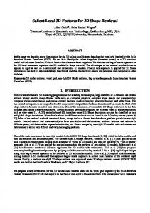
2.7. Examples Tab. 1 shows processes of the shape-distribution based method using examples. We use a teapot, a sphere and a mechanical part as sample models. We first triangulate these models into triangle sets. Then, we use Halton’s QRNS to generate sample points. After then D2 distributions [23] and AAD distributions [20] are generated based on these sample points. A Teapot

A Sphere

A Part

3D Model

Triangle Set

Sample Points

D2 Distribution

AAD Distribution

Tab. 1: D2 Distributions and AAD distributions. 3. DISCUSSIONS 3.1. Discriminability Shape distribution-based methods are easy for implementation, and easy for both of offline indexing operation and online matching operation. Most of them have remarkable advantage of low

Computer-Aided Design & Applications, 6(5), 2009, 721-735

730

computational cost. Accordingly, shape distribution-based methods are suitable for a coarse filter of a 3D shape retrieval system. The obvious limitation of original Osada’s D2 Method is that very different 3D shapes may have close distance, in other words, this method has not enough discriminating capability, because the features carried by 64 vectors are too limit. Simply increasing the number of vectors by reducing the bin-width and increasing sample counts accordingly may improve the discriminability, but it also increasing the comparison cost and the storage. All methods based on Osada’s D2 are engaged in increasing the discriminability of D2 with same computational cost or by slightly increasing computational intensity. The Osada’s D2 is considered as too simple and losing too many detailed features. As the result, the aim is to enhance Osada’s D2 with additional dimensions of 64 vectors for more detailed features. 3.2. Sample Counts The approach proposed by Ip et al [9], [10] is to classify the distances between pairs of sample points into three categories: IN, OUT and MIXED. Both Rea and Iyer [11], [26] pointed out that its computational cost is considerably high, because it involves a large number of intersection calculation. This computational intensity may be sharply aggravated while increasing the number of polygons or triangles. The insufficiency of sample counts is also a problem in Ip’s method [9], [10]. Although the total number of sample points seems adequate, the assignment of the sample counts in the three categories (IN, OUT and MIXED) is extremely unbalanced. In order to solve this problem, one way is conditionally sampling, but it is very complicated in this context. The other way is to increase the total number of samples, but it will ulteriorly increase the computational cost and the total number of samples is not able to be determined before the sampling process. 3.3. Weighted Distance Another question is that if a feature is only carried by less than 1% population of samples, is it still a major feature of this 3D model? For example, if we constantly reduce the diameter of the caves in the cheese model shown in Fig. 8, the population of the OUT and MIXED will also be decreased. At the same time, the re-entrant feature of this model will become less important, and finally become a trivia.

Fig. 8: Cheese Model [9]. Subsequently, the feature effects in 3D shape matching are dynamic, when the features are compound together into a single descriptor. Both Ip et al [9] and Ohbuchi et al [21] were aware with this issue. Ip tried three different weighting methods to adjust the effects of IN, OUT and MIXED distributions, but these methods seems not working as well as expected. Ohbuchi also tried several different set of weights to compound the features together, and chose the one with best performance as their result. Ip et al [10] changed their tactics into using another method to determine the weights by training the classification system. The weights of IN, OUT and MIXED distributions are same in one 3D shape category and differs between categories. This is reasonable, because the shapes in one category are supposed to have same major features, and one feature may have different importance in different categories. For example, the concave feature is one of most important features in cheese-like models, but for a cube, it is not important at all. Computer-Aided Design & Applications, 6(5), 2009, 721-735

731

3.4. Feature Redundancy Rea et al [26] roughly stated how the distributions of faces can be combined together into a distribution of 3D shape. For example, as qualitatively shown in Fig. 9, the probability distribution of a cube can be viewed as a combination of the probability distribution of individual faces, pair of orthogonal faces, and pairs of parallel faces.

Fig. 9: Constituent parts of cube D2. Here we prefer to discuss it in a quantitative manner to infer another interesting topic. When we consider two random sample points on the surface of a cube with edge length of a, there might be one of three possible relationships between them: 1) they are located in a same face; 2) they are located in different faces, and the two faces are orthogonal; 3) they are located in different faces, and the two faces are parallel. The probabilities of the three possible events are P (1)  1 , P(2)  2 , and P (3)  1 , respectively. Then 6 3 6 we process a conditional sampling to get the D2 distribution of these three conditions, which are denoted as f (1) , f (2) and f (3) . As shown in Fig. 10, these distributions are supposed to be normalized with same bin-width:

3a

64

.

Fig. 10: Three probability distributions for the three given conditions.

Computer-Aided Design & Applications, 6(5), 2009, 721-735

732

The probability distributions of orthogonal faces and parallel faces shown in Fig. 10 are different from those shown in Fig. 9, because in Rea’s experiment [26], the events of two sample points in a same face were not eliminated from the cases of orthogonal faces and parallel faces.

Fig. 11: (a) The compound distribution, and (b) D2 distribution of a cube. We combine the three probability distributions with the weight as the three events probability, P  , 1

P

2

and P

 3

. The compound probability distribution denoted as f f j c  

3

1

2

1

 P  f    6 f    3 f    6 f   , k

k

j

1

2

j

j

3

j

c

can be calculated as:

j  1,2,...,64

(11)

k 1

As shown in Fig. 11, we finally get the compound probability distribution which is utterly as same as the D2 distribution of a cube. As the sampling is area weighted, the formula (11) can be generalized to a uniform form. In a 3D i i ij model, the area of a polygon S    S is denoted as A  , and f   is the probability distribution when

the first random sample point is located in S   and the second random sample points is located in i

j S   . Then the D2 distribution of this 3D model can be expressed as:

n

n

 A  A  f   i

ij

j

k

fk 

i 1 j 1

, k  1, 2,..., m (12) A Where A is the total area of the polygon set S , m is the number of vectors and n is the number of polygons. In a specific case, when two subsets, G  S and H  S , are complement sets for S : G  H , the total area of G is AG , and the total area of H is AH . The distribution of the universal set S can be calculated as:

f 

1

 AG  AH 2

A

2 G fGG

 2 AG AH fGH  AH2 f HH

Computer-Aided Design & Applications, 6(5), 2009, 721-735



(13)

733

Where fGG is the D2 distribution of subset G , f HH is the D2 distribution of subset H , and fGH is the D2 distribution when the first random sample point is located in G and the second random sample point is located in H . The formula (13) illuminates that the D2 distribution of any 3D model S , can be expressed as a linear combination of the D2 distribution of the subsets of S . This formulation could be used to determine the redundant feature, when we approach to increasing dimensions of descriptors by decomposing the 3D model into several subsets with specific features. In some circumstances, we would rather express a distance between a linear combination of the weighted distance between the subsets. This technique will substantially enhance the discriminability by increasing the dimension counts of the descriptors. Yet, the ways to determine the weights have to be concerned with. 3.5. Extending Dimension of Descriptors The approach used by Rea et al [26] seems having a very close relationship to formula (13), but Rea’s method is actually more likely a specific case of AMRR proposed by Ohbuchi et al [21]. Ohbuchi incorporated weighted distances between the alpha shapes into the distance between original models to increase the descriptor’s capability. When there is only one level of alpha shape in Ohbuchi’s AMRR, and the parameter  is  , the case in Ohbuchi’s AMRR will become the same as Rea’s method. Instead of combining the weighted distance between the alpha shapes and the distance between the original models, Rea’s method is to subtract the D2 distribution directly from the D2 distribution of the original models. The physical meaning of Rea’s distribution is the distance between the distributions of the original 3D model and the convex hull of its own, in other words, Rea’s distance is ‘distance between distances’. This disposal actually does not increase the capability of the descriptors. It just transforms the descriptors carrying some features into the descriptors carrying some other features. In an extreme case, for instance, when the original model is a convex model, the CHD distribution will become value zero. That is, the approach proposed by Rea et al [26] can only be applied to the models with reentrant features. And unfortunately, in Rea’s method, the negative values are ignored, but these negative values also carry features with them and should not be rejected. AD, ADD and AMRR proposed by Ohbuchi et al [20], [21] successfully extended Osada’s D2 distribution into a multi-dimensional space. However, they use inner products of the unit normal vectors of triangles which the pairs of sample points are located on as another dimension, and it is divided equally into 8 intervals.

Fig. 12: Angle intervals corresponding to the inner product intervals. As shown in Fig. 12, supposing that the angles between pairs of faces are uniformly distributed in 0,   , because the cosine function is not a linear function, the assignment of sample counts in the 8

Computer-Aided Design & Applications, 6(5), 2009, 721-735

734

intervals on inner products is not balanced. The intervals of  1.0, 0.75 and  0.75,1.0 will get more samples than other intervals, and accordingly, some of the detailed features of the approximately parallel triangles will be concealed. Liu et al [15] used a statistical ‘thickness’ histogram as the descriptor of 3D shapes. Their method is roughly similar as Osada’s D2, but when a distance between a pair of sample points falls into a histogram bin, the bin’s value will be added with a weight W instead of value 1: dot  n, n1  dot  n, n2  w (14) d2 Where the dot   denotes the inner product of two vectors, and n is the unit vector along the line segment between the sample points, n1 and n2 are the unit normal vectors of the triangles on which the pair of sample points are located. It is hard to find out the physical meaning of this weight. The factor of 1 2 causes the first bins in the histogram rather unstable. d 4. CONCLUSIONS Most methods of the shape distribution-based 3D shape retrieval are fast and efficient for 3D shape matching. Although their discriminating capability cannot compete with the more elaborate features (for instance, spherical harmonics in Kazhdan et al [13]), they are suitable for working as coarse filters in 3D shape search engines because of their low computational cost. Several approaches were proposed to increase the discriminability of Osada’s D2. By analyzing their work, we can indicate the direction of future research for improving the performance of Osada’s D2. First of all, the discriminating capability can be enhanced by increasing dimensions of vectors, because the feature capability of the 64 vectors in Osada’s D2 is too limited. One way to increase the dimension of vectors is to classify the triangles into several categories with different features. The other way is to incorporate other features into the descriptors as additional dimension, as Ohbuchi did in the AD, AAD and AMRR approaches. Secondly, distances should be expressed as sums of weighted components along the dimensions. The distance between 3D models should be a form of linear combination of features. The feature with maximum weight is the major feature. Generally speaking, different categories might have different weights of same feature because their major features are different from each other. Setting the weights of these categories by using data mining methods should be considered. 5. REFERENCES [1] Alt, H.; Guibas, L.-J.: Discrete geometric shapes: Matching, interpolation, and approximation, Handbook of Computational Geometry, 1996. [2] Arya, S.; Mount, D.-M.; Netanyahu, N.-S.; Silverman, R.; Wu, A.-Y.: An optimal algorithm for approximate nearest neighbor searching fixed dimensions, JACM, 45(6), 1998, 891-923. [3] Chazelle, B.: Triangulating a simple polygon in linear time, Discrete and Computational Geometry, 6(1), 1991, 485-524. [4] Chi, H.; Mascagni, M.; Warnock, T.: On the optimal Halton sequence, Mathematics and Computers in Simulation, 70(1), 2005, 9-21. [5] Circle Line Picking, http://mathworld.wolfram.com/CircleLinePicking.html, Wolfram Mathworld. [6] Funkhouser, T.; Min, P.; Kazhdan, M.; Chen, J.; Halderman, A.; Dobkin, D.; Jacobs, D.: A search engine for 3D models, ACM Trans.Graph., 22(1), 2003, 83-105. [7] Funkhouser, T.; Kazhdan, M.; Shilane, P.; Min, P.; Kiefer, W.; Tal, A.; Rusinkiewicz, S.; Dobkin, D.: Modeling by example, SIGGRAPH '04: ACM SIGGRAPH 2004 Papers, 2004, 652-663. [8] Halton, J.-H.: On the efficiency of certain quasi-random sequences of points in evaluating multidimensional integrals, Numerische Mathematik, 2(1), 1960, 84-90. [9] Ip, C.-Y.; Lapadat, D.; Sieger, L.; Regli, W.-C.: Using shape distributions to compare solid models, SMA '02: Proceedings of the Seventh ACM Symposium on Solid Modeling and Applications, 2002, 273-280. Computer-Aided Design & Applications, 6(5), 2009, 721-735

735

[10] [11] [12] [13] [14] [15] [16] [17] [18] [19] [20] [21] [22] [23] [24] [25] [26] [27] [28] [29]

Ip, C.-Y.; Regli, W.-C.; Sieger, L.; Shokoufandeh, A.: Automated learning of model classifications, SM '03: Proceedings of the Eighth ACM Symposium on Solid Modeling and Applications, 2003, 322-327. Iyer, N.; Jayanti, S.; Lou, K.; Kalyanaraman, Y.; Ramani, K.: Three-dimensional shape searching: state-of-the-art review and future trends, Comput. -Aided Des., 37(5), 2005, 509-530. Kazhdan, M.; Chazelle, B.; Dobkin, D.; Finkelstein, A.; Funkhouser, T.: A reflective symmetry descriptor, Computer Vision - ECCV 2002, 2002, 777-778. Kazhdan, M.; Funkhouser, T.: Harmonic 3D shape matching, SIGGRAPH '02: ACM SIGGRAPH 2002 Conference Abstracts and Applications, 2002, 191-191. Kazhdan, M.; Funkhouser, T.; Rusinkiewicz, S.: Rotation invariant spherical harmonic representation of 3D shape descriptors, SGP '03: Proceedings of the 2003 Eurographics/ACM SIGGRAPH Symposium on Geometry Processing, 2003, 156-164. Liu, Y.; Pu, J.; Zha, H.; Liu, W.; Uehara, Y.: Thickness histogram and statistical harmonic representation for 3D model retrieval, International Symposium on 3D Data Processing Visualization and Transmission, 2004, 896-903. Min, P.; Chen, J.; Funkhouser, T.: A 2D sketch interface for a 3D model search engine, SIGGRAPH '02: ACM SIGGRAPH 2002 Conference Abstracts and Applications, 2002, 138-138. Min, P.; Halderman, J.-A.; Kazhdan, M.; Funkhouser, T.-A.: Early experiences with a 3D model search engine, Web3D '03: Proceedings of the Eighth International Conference on 3D Web Technology, 2003, pp. 7-18. Min, P.; Kazhdan, M.; Funkhouser, T.: A Comparison of text and shape matching for retrieval of online 3D models, Research and Advanced Technology for Digital Libraries, 2004, 209-220. Ohbuchi, R.; Otagiri, T.; Ibato, M.; Takei, T.: Shape-similarity search of three-dimensional models using parameterized statistics, 2002, 265- 274. Ohbuchi, R.; Minamitani, T.; Takei, T.: Shape-similarity search of 3D models by using enhanced shape functions, TPCG '03: Proceedings of the Theory and Practice of Computer Graphics 2003, 2003, 97-104 Ohbuchi, R.; Takei, T.: Shape-similarity comparison of 3D models using alpha shapes, PG '03: Proceedings of the 11th Pacific Conference on Computer Graphics and Applications, 2003, 293302. Osada, R.; Funkhouser, T.; Chazelle, B.; Dobkin, D.: Matching 3D models with shape distributions, Proceedings International Conference on Shape Modeling and Applications, 2001, 154-66. Osada, R.; Funkhouser, T.; Chazelle, B.; Dobkin, D.: Shape distributions, ACM Transactions on Graphics, 21(4), 2002, 807-32. Pu, J.; Liu, Y.; Xin, G.; Zha, H.; Liu, W.; Yusuke, U.: 3D model retrieval based on 2D slice similarity measurements, Second International Symposium on 3D Data Processing, Visualization and Transmission (3DPVT'04), 2004, 95-101 Pu, J.; Ramani, K.: An integrated 2D and 3D shape-based search framework and applications, Computer-Aided Design and Applications, 4(1-6), 2007, 817-826. Rea, H.-J.; Sung, R.; Corney, J.; Clark, D.: Identifying three-dimensional object features using shape distributions, Computer Aided Production Engineering - CAPE 2003, 2003, 23-32. Rea, H.-J.; Clark, D.-E.-R.; Corney, J.-R.; Taylor, N.-K.: A surface partitioning spectrum (SPS) for retrieval and indexing of 3D CAD models, Second International Symposium on 3D Data Processing, Visualization and Transmission (3DPVT'04), 2004, 167-174 Press, W.-H.; Teukolsky, S.-A.; Vetterling, W.-T.; Flannery, B.-P.: Numerical Recipes in C (2nd Ed.): The Art of Scientific Computing, Cambridge University Press, New York, NY, USA, 1992. Tangelder, J.; Veltkamp, R.: A survey of content based 3D shape retrieval methods, Multimedia Tools Appl, 39(3), 2008, 441-471.

Computer-Aided Design & Applications, 6(5), 2009, 721-735