Coverage Diameters of Polygons Pawin Vongmasa
Attawith Sudsang
Department of Computer Engineering Chulalongkorn University Bangkok, Thailand 10330 Email:
[email protected]
Department of Computer Engineering Chulalongkorn University Bangkok, Thailand 10330 Email:
[email protected]
Abstract— This paper formalizes and proposes an algorithm to compute coverage diameters of polygons in 2D. Roughly speaking, the coverage diameter of a polygon is the longest possible distance between two points through which the polygon cannot pass in between. The primary use of coverage diameter is to form a cage for transporting an object, not necessarily convex, with multiple disc-shaped robots. The main idea of the computation of coverage diameter is to convert the problem into a graph structure, then perform the search for a solution path in that graph. The proposed algorithm runs in O(n2 log n) time for the input polygon with n vertices.
I. I NTRODUCTION To cage an object means to limit object’s configuration space to a bounded subset. Many types of caging problems have been raised, but the one that has been studied most extensively is how to form a cage by a number of point obstacles in R2 . Solutions to this problem can be applied quite directly to transportation of an object by multiple disc-shaped robots: form a cage by robots, then move them together at the same velocity. In practice, it is difficult to synchronize multiple robots to move together at exactly the same velocity, so if we are to transport an object by putting it in a moving cage formed by these robots, the cage should be allowed to deform a bit. This paper presents a new sufficient caging condition for this situation that is easy to maintain — it requires only that each robot can keep the distances from itself to its nearby friends under a predetermined value, which will be called “coverage diameter”. Roughly speaking, the coverage diameter of a rigid simple closed curve in R2 is the shortest length of gap (space between two points) that allows the curve to pass through. Therefore, the curve cannot escape from surrounding points, and is said to be caged, if every surrounding gap is smaller than the coverage diameter. The notion of caging was first introduced in [1]. The problem of determining the caging set for 2-fingered gripping systems with one degree of freedom in the plane was studied in [2]. The extension to 3-fingered gripper, also with one degree of freedom, was explored in [3]. Caging in these works serves as a quick pre-process toward immobilizing grasp. Errortolerance was added in [4]. Later in [5], a way to produce v-grips at concave vertices using two fingers was presented. Once two fingers form a v-grip, they can move inward or outward by some distance
while preserving the caging condition. The maximum amount of distance that keeps the cage can be computed by the method presented in [6]. Note that in some cases (such as convex polygons) where no v-grips exist, surrounding points that satisfy our coverage diameter condition can serve as a complementary cage. Manipulating polygonal objects using three 2-DOF robots, proposed in [7], involved caging as a transition between different form closures. The need of form closures was relaxed with the help of MICaDs (maximum independent capture discs) introduced in [8]. Then, motion planning and caging were combined in [9]. Nonetheless, these methods are applicable only to the case of three robots with high functionalities. Cages of more than three robots were discussed in [10]. The notion of object closure was introduced and used in stating a sufficient and necessary condition for caging, but the test to verify object closure involves complicated operations and is extremely time-consuming. An alternative test method which takes less time was also presented in [10], but its completeness was not guaranteed. Presented in [11] is a new sufficient condition for caging which is, though as well incomplete, much easier to check and more practical in many situations. It involves the calculation of diameter function of convex polygons, which was first brought up in [12]. However, the sufficient condition stated in [11] can be both tightened and simplified with the meaning of coverage diameter. The improved condition is stated in Section II after an intuitive definition of coverage diameter is discussed. In Section III, we introduce related terms, redefine coverage diameter formally, and state lemmas that are needed in the computation of coverage diameter of polygons. The idea of the computation involves formulating the problem into a graph structure. Such formulation is explained in Section IV. Finally, the pseudocode of the algorithm and some experimental results are shown in Section V. II. C OVERAGE D IAMETER AND C AGING C ONDITION Imagine an object in a cage formed by points. If the object is about to escape the cage, it must get through a gap between some two points of the cage. Our original goal is to find the largest separation distance between points such that the object cannot escape. But in reality, when we try to transport the object by forming a moving cage with mobile robots, distances among
them cannot easily be kept constant as they move. It is more practical to allow some distance change and maintain only the upper bound of separation distance. We call this upper bound value the coverage diameter and denote it by φcov (C) if the curve is C. A new sufficient condition for C to be caged by surrounding points is immediate from the notion of φcov (C). Lemma 1: Let P be a polygon with vertices P1 , P2 , P3 , ..., Pn ∈ R2 arranged counterclockwise and let P0 = Pn . If C is a rigid closed curve that lies inside P and kPi − Pi−1 k < φcov (C) where i ∈ {1, 2, 3, ..., n}, then C is caged by {P1 , P2 , P3 , ..., Pn }. Note that the cage formed by surrounding points can contain more than one objects provided that all separation distances are smaller than the minimum coverage diameter of all objects (Fig. 2).
f inal(Z) = d is called the final point of Z, and graph(Z) = A is called the graph of Z. Motion of a point will be represented by a directed arc because magnitude of velocity is not relevant to our discussion. Next, we will consider the paired motion of two points together because a gap in R2 is defined by two points. Definition 2: Let V be a Euclidean space. 1) If a ∈ V and b ∈ V , the inner distance of (a, b) ∈ V 2 is k(a, b)kin = ka − bk. 2) If A ⊆ V 2 , the maximum inner distance of A is kdAekin = max{kakin | a ∈ A}. Similarly, the minimum inner distance of A is kbAckin = min{kakin | a ∈ A}. A. Coverages and the Coverage Diameter
coverage diameter
longer than coverage diameter
(a)
(b)
longer than coverage diameter (c)
Fig. 1. The condition is sufficient but not necessary. (a) The object is caged because all gaps are smaller than the coverage diameter. (b) The object may escape when there is a gap larger than the coverage diameter. (c) The object cannot escape despite the presence of a gap larger than the coverage diameter.
Imagine when C is being pushed through a gap between two points a and b in R2 . The situation will be viewed from a-b’s frame of reference where a is the origin and b is on the positive-y axis. Note that b is allowed to move up and down along the positive-y axis. In the initial set up, let C lie totally in the left half plane. Every point of C has an integer called the coverage count attached to it. All coverage counts are initially zero. At any instant, the cross section is the part of C that intersects the straight line segment drawn from a to b. If a point of C is in the cross section and is moving into the right half plane, the coverage count of that point is increased by 1. Oppositely, the coverage count is decreased by 1 if it is moving into the left half plane. b
(a)
Fig. 2. Shown in dotted lines are coverage diameters. All objects are caged because all gaps are smaller than the shortest coverage diameter.
III. F UNDAMENTALS Definition 1: An arc is a connected set of points homeomorphic to the closed interval [0, 1]. A directed arc is a triple Z = (A, s, d) where A is an arc, s is an endpoint of A, and d is the other endpoint of A. initial(Z) = s is called the initial point of Z,
b
b
+
−
−
+
−
+
a
a
a
(b)
(c)
Fig. 3. (a) The object is moving to the right. Coverage counts of points in the cross section will increase by 1. (b) The object is moving to the left. Coverage counts of points in the cross section will decrease by 1. (c) The object is rotating around a point (not shown). Coverage counts of points in the cross section may decrease or increase depending on the position of the fixed point.
When the whole motion is known, a point of C starts to be covered at the last moment its coverage count changes from 0 to 1. Once a point becomes covered, it remains covered for the rest of the motion (Fig. 4). When all coverage counts are equal to 1, C is said to be covered by the paired motion of a and b viewed from C’s frame of reference. Such paired motion can be represented by a directed arc in R4 that is called a coverage of C.
Coverage Count
b0
b02
b
b
a0
(a) 2 1
1
1
0
a0
φcov (C) (a)
(b)
(c)
End of Motion b
0
b01
b0
the point is COVERED
0
b
Time
0
a0
b
0
a0
Not yet COVERED b
(d)
(b)
then
a
(e)
Fig. 5. (a) Some snapshots of Z. (b) Covered points in some cross sections are shown in white. a0 and b0 are the farthest pair in K, i.e. k(a0 , b0 )kin = kdK 2 ekin . (c) The point of discontinuity: (a0 , b01 ) and (a0 , b02 ) are different limits. (d-e) A directed arc in U that fixes the discontinuity.
a
Fig. 4. (a) The point starts to be covered at the moment its coverage count increases from and never decreases to 0. If we know that the point is eventually covered, it is possible to view backward (from right to left) and marks the point as uncovered once its count reaches zero. (b) An example of not-yetcovered points in the real situation.
The maximum inner distance of a coverage is equal to the maximum separation distance between a and b during the motion. It is obvious that the smallest maximum inner distance of all coverages is exactly the same as coverage diameter we have mentioned. Definition 3: If C is a simple closed curve in R2 , its coverage diameter is φcov (C) = min{kdgraph(Z)ekin | Z is a coverage of C} Note that there are infinitely many coverages whose maximum inner distances are equal to φcov (C). We need to find just one of them. B. Boundary Coverages A coverage Z of C is called a boundary coverage if 1) graph(Z) ⊆ C 2 2) kinitial(Z)kin = kf inal(Z)kin = 0 We claim that there always exists a boundary coverage whose maximum inner distance is equal to φcov (C). This fact allows us to limit the search to boundary coverages only. To prove the claim, let Z be a coverage with kgraph(Z)kin = φcov (C) (Fig. 5.a). At each instant of the motion that constitutes Z, let a and b be the two moving points and let K be the set of points in the cross section that are “covered” (as in Fig. 4) at that time. It is obvious that kdK 2 ekin ≤ φcov (C) for all K. Let U be the union of all K 2 , written as: [ U = K2 all K
It is again obvious that kdU ekin = φcov (C).
Next, let a0 and b0 be two new moving points in K that are closest to a and b (Fig. 5.b). We know that (a0 , b0 ) ∈ U but a0 and b0 might not be continuous with respect to time (Fig. 5.c). However, these discontinuities can be filled by directed arcs in U whose initial and final points are the different limits (Fig. 5.d, 5.e). These directed arcs always exist because U is connected due to the fact that once a point is covered, it remains covered through the rest of the motion. Therefore, the paired motion (a0 , b0 ) with all discontinuities removed composes a coverage whose graph is a subset of U ⊆ C 2 . Combining this result with the fact that (p, p) ∈ U for all p ∈ C, the coverage just described can be extended such that its initial and final points have zero inner distance. If we let the initial point be any member of the first non-empty K 2 and the final point be any member of the last non-empty K 2 , the result of this extension becomes a boundary coverage. Our claim is now proved and we summarize it in the following lemma. Lemma 2: For a given simple closed curve C ⊂ R2 , there always exists a boundary coverage Z such that kdgraph(Z)ekin = φcov (C). Proof: The above remark constitutes a proof. C. Line Segments A line segment is a special kind of arcs whose points can be written as a linear function of one variable. Line segments will be involved when we work with polygons, a special kind of simple closed curves. The following lemma assumes that distance of a point is measured from the origin. Lemma 3: If p and q are the two endpoints of a line segment L, max{kxk | x ∈ L} = max{kpk, kqk}. Proof: If kpk ≥ kqk, the circle with radius kpk centered at the origin will contain L; therefore, max{kxk | x ∈ L} = kpk. The other case where kpk < kqk is proved by exchanging p and q. Directed arcs whose graphs are line segments are called directed line segments. The following lemma shows an impor-
tant characteristic of paired directed line segments that will be used in the next section. Lemma 4: Given two directed line segments X and Y in R2 , if Z is a line segment in R4 whose endpoints are (initial(X), initial(Y )) and (f inal(X), f inal(Y )), then
Vi
Vi
Ej Pi,j
kdZekin
max{kinitial(X) − initial(Y )k, kf inal(X) − f inal(Y )k} Proof: See Appendix. =
IV. C OMPUTATION OF φcov (C) We are going to find the coverage diameter of the polygon C ⊆ R2 that has n vertices and n edges, namely Vi and Ei where i ∈ Zn 1 . Vi are ordered counterclockwise. Every Ei is a line segment in R2 with endpoints Vi and Vi+1 . To find φcov (C), we will construct a graph G that contains enough information of C, then perform a search in G. The steps toward construction of G are outlined below: 1) We will define subsets of C 2 called states. Every point of C 2 will belong to exactly one state. 2) Every directed arc in C 2 will have a corresponding state sequence. We will show that it is adequate to consider only state sequences without looking at any corresponding directed arcs. 3) Initial and final states will be defined by examining state sequences of boundary coverages. 4) Some states will be chosen to become nodes of G and we will derive edges of G from state adjencies. After G is completely defined, the algorithm to find φcov (C) will be presented. A. States The following subsets of C 2 for all i, j ∈ Zn are called states: • Vi Vj = {(Vi , Vj )} • Vi Ej = {Vi } × Ej • Ei Vj = Ei × {Vj } • Ei Ej = E i × Ej Note that the union of all states is C 2 . Let bXcin denote the point of a state X with smallest inner distance. If there are more than one points with equal inner distance, we can choose any one of them. Note that kbXckin (from Definition 2) is equal to the inner distance of bXcin . We need to know bXcin of all states X. For states of the form Vi Vj , it is obvious that bVi Vj cin = (Vi , Vj ). Next, if we let Pi,j be projections 2 of Vi on Ej , then bVi Ej cin = (Vi , Pi,j ) and bEi Vj cin = (Pj,i , Vi ). In order to find bEi Ej cin , it is easy to show that bEi Ej cin must be equal to at least one of these four points: bVi Ej cin , bVi+1 Ej cin , bEi Vj cin and bEi Vj+1 cin . Three comparisons will give the correct value of each bEi Ej cin . 1Z n is a group of non-negative integers less than n. Additions and subtractions are calculated modulo n. 2 In this context, the projection of a point p on a set S is the point of S closest to p. With this definition, the projection must exist and be unique given that S is a line segment.
Ej Pi,j
(a)
(b)
Fig. 6. The line segment Vi Pi,j may or may not be perpendicular to Ej . (a) Vi Pi,j is perpendicular to Ej . (b) Vi Pi,j is not perpendicular to Ej and Pi,j coincides with Vj or Vj+1 .
B. State Sequences For a given directed arc Z in C 2 , let σ(Z) be the sequence of states that points of Z belong to. Here arises one problem: a point of C 2 may be a member of more than one states. We will try to choose states of the form Vi Vj first, Vi Ej and Ei Vj next, then Ei Ej . As “belong to” is defined this way (different from “∈”), the function σ(Z) is now clearly defined. Let S be a finite state sequence of length m: S = (S1 , S2 , S3 , ..., Sm ) The maxi-min inner distance of S is kdbScekin = max{kbSi ckin | i = 1, 2, 3, ..., m} It is easy to show that kdgraph(Z)ekin ≥ kdbScekin whenever σ(Z) = S. Two states X and Y are adjacent if and only if the state sequence (X, Y ) exists. All state adjacencies are listed below: • States adjacent to Vi Vj : Ei Ej , Ei Ej−1 , Ei−1 Ej , Ei−1 Ej−1 , Vi Ej , Vi Ej−1 , Ei Vj and Ei−1 Vj • States adjacent to Vi Ej : Ei Ej , Ei−1 Ej , Vi Vj and Vi Vj+1 • States adjacent to Ei Vj : Ei Ej , Ei Ej−1 , Vi Vj and Vi+1 Vj • States adjacent to Ei Ej : Vi Vj , Vi Vj+1 , Vi+1 Vj , Vi+1 Vj+1 , Vi Ej , Vi+1 Ej , Ei Vj and Ei Vj+1 We are going to show that if X and Y are adjacent states, then bXcin ∈ X ∩ Y or bY cin ∈ X ∩ Y . Since Vi Ej are not adjacent to any Vk El or Ek Vl , it suffices to consider only these cases: • If X = Vi Vj : X ⊆ Y , so bXcin ∈ X ∩ Y . • If X = Ei Ej : Y ⊆ X, so bY cin ∈ X ∩ Y . This means if X and Y are adjacent states, there always exists a directed arc Z such that σ(Z) = (X, Y ) and kdZekin = max{kbXckin , kbY ckin }. We also know that all states are convex subsets of R4 , which means once a point enters a state Si , it can move to bSi cin in a straight line motion. Therefore, when the state sequence S is given, it is always possible to find Z such that σ(Z) = S and, with the help of Lemma 4, kdZekin = kdbScekin .
C. Initial and Final States Imagine the paired motion of two points (a, b) that constitutes a boundary coverage Z again, the constraint “kinitial(Z)kin = kf inal(Z)kin = 0” requires that the two points start from one initial point, split in opposite directions relative to each other, then meet again at one final point. Without loss of generality, we can assume two things: • a and b do not cross during the whole time except at the initial and final points. • When a and b split and meet, a is moving in the clockwise direction relative to b. Every state that contains a point of the form (p, p) can act as both an initial state and a final state. All states that has (p, p) are: Vi Vi , Vi Ei , Vi Ei−1 , Ei Vi , Ei−1 Vi , Ei Ei , Ei Ei+1 and Ei Ei−1 . We will look more closely at this matter after states become nodes of G. D. The Graph G From all the above discussions, it seems rather clear how G should be constructed: states become nodes, transitions become edges, and state sequences become paths. The idea of the algorithm is also simple: find a state sequence that starts from one initial state, ends at one final state, and has the smallest maxi-min inner distance. This simple idea actually works, but there are numerous redundancies that should be removed for efficiency. Start by looking at Ei Ej . It is obvious that all minimum inner distances of states adjacent to Ei Ej are never smaller than kbEi Ej ckin . This means if X and Y are states adjacent to Ei Ej , kbEi Ej ckin can be excluded from the calculation of maxi-min inner distance of (X, Ei Ej , Y ). With another observation that adjacent states of Ei Ej are NOT of the form Ek El , all Ei Ej can be removed from every sequence as they are subsumed by adjacent states. Next, consider states of the form Vi Vj . Before Ei Ej are removed, all states adjacent to Vi Vj are not of the form Vk Vl , but once we bypass Ei Ej , Vi Vj can jump to some Vk Vl . Still, we can manage to insert some states of the form Vi Ej or Ei Vj in between and reduce some adjacencies. Look at the state sequence (Vi Vj , Ei Ej , Vi+1 Vj+1 ). The corresponding path with Ei Ej removed is Vi Vj → Vi+1 Vj+1 We know that intermediate states (adjacent to Vi Vj and Vi+1 Vj+1 ) are Vi Ej , Ei Vj , Vi+1 Ej and Ei Vj+1 , all of which have minimum inner distances not exceeding max{kVi − Vj k, kVi+1 −Vj+1 k}. Inserting any of them in the middle does not increase the maxi-min inner distance of the path, so we do so Vi Vj → Vi Ej → Vi+1 Vj+1 All the other cases, such as (Vi Vj , X, Vi Vj+1 ), can be handled by similar arguments. Edges of G, then, do not have to include V i Vj → V k Vl .
We now revisit the problem of specifying initial nodes and final nodes. From the previous discussion, nodes that may act as initial and final nodes are: Vi Vi , Vi Ei , Vi Ei−1 , Ei Vi and Ei−1 Vi . We want to assign each of them as initial or final only, but not both. • Vi Ei should be declared initial because (p, q) belongs to Vi Ei implies that p = Vi and q lies in the counterclockwise direction from p (due to our restriction of the counterclockwise arrangement of Vi ). • Vi Ei−1 should be declared final because (p, q) belongs to Vi Ei−1 implies that p = Vi and q lies in the clockwise direction from p. • Ei Vi should be declared final because Vi Ei are initial. • Ei−1 Vi should be declared initial because Vi Ei−1 are final. • Vi Vi can be removed because all nodes adjacent to Vi Vi have already been declared initial or final. We are now ready to list all nodes and edges of G as follows: 1) From Vi Ei : Vi−1 Ei , Vi Vi+1 and Ei−1 Vi+1 2) From Ei−1 Vi : Vi−1 Vi , Vi−1 Ei and Ei−1 Vi+1 3) From Ei Vi : Ei Vi−1 , Vi+1 Vi and Vi+1 Ei−1 4) From Vi Ei−1 : Vi Vi−1 , Ei Vi−1 and Vi+1 Ei−1 5) From Vi Vj , i 6= j: Vi Ej , Vi Ej−1 , Ei Vj and Ei−1 Vj 6) From Vi Ej , i 6= j and i 6= j + 1: Ei Vj , Ei Vj+1 , Ei−1 Vj , Ei−1 Vj+1 , Vi Vj and Vi Vj+1 7) From Ei Vj , i 6= j and i 6= j + 1: Vi Ej , Vi+1 Ej , Vi Ej−1 , Vi+1 Ej−1 , Vi Vj and Vi+1 Vj (1) and (2) are from initial nodes. (3) and (4) are from final nodes. (5), (6) and (7) are from internal (neither initial nor final) nodes. The total number of nodes is 3n2 − n and the total number of edges is 8n2 − 8n. To find φcov (C), we need to search for a path S in G that starts from an initial node, ends at a final node, and has the smallest maxi-min inner distance. Once S is found, a boundary coverage Z of C such that σ(Z) = S and kdgraph(Z)ekin = kdbScekin always exists. V. A LGORITHM Our goal is to find a path S in G that covers C, i.e. starts from an initial node and ends at a final node. The characteristic of maxi-min inner distance of paths allows us to apply the idea from Dijkstra’s shortest path algorithm. The pseudocode of the algorithm is shown in Fig. 7. Note that if max{d, kbtckin } in line (11) is replaced by d + [distance of s → t], the pseudocode becomes exactly the shortest path algorithm. The running time of this algorithm is accordingly O(n2 log n). The algorithm has been implemented in C++ and tested on 1.5 GHz CPU with 512 MB RAM. It could process the input polygon with 1000 vertices within 3 seconds. Some visual experimental results are shown in Fig. 8.
(1) (2) (3) (4) (5) (6) (7) (8) (9) (10) (11) (12) (13) (14) (15) (16) (17) (18) (19)
Let V isited be a set, initially empty, for storing visited nodes. Let H be a min-heap, initially empty, for storing a couple (d, s) where d is a real number used in comparison and s is a node of G. For each initial node s, add (0, s) to H. Repeat the following until φcov (C) is found: begin Retrieve and remove the minimum couple (d, s) from H. Add s to V isited. If s is a final node, report that φcov (C) = d and terminate. For each t ∈ / V isited such that edge s → t exists, begin Let m = max{d, kbtckin }. If there exists a couple (e, t) in H for some e, then begin If m < e, replace (e, t) in H by (m, t) and adjust H. Else, do nothing. end. Else, add (m, t) to H. end. end. Fig. 7.
The pseudocode of our searching algorithm.
A PPENDIX Proof of Lemma 4 Proof: The existence and uniqueness of Z follow at once as its two endpoints are specified. It is possible to let points in X, Y and Z be formulated as linear functions of the same variable t ∈ [0, 1] as follows: X(t) Y (t) Z(t)
= = =
(1 − t) · initial(X) + t · f inal(X) (1 − t) · initial(Y ) + t · f inal(Y ) (X(t), Y (t))
Let W (t) = X(t)−Y (t); it follows that the graph of W (t) where 0 ≤ t ≤ 1 is a line segment in R2 with endpoints X(0) − Y (0) and X(1) − Y (1). From Lemma 3, we have that max{kW (t)k | 0 ≤ t ≤ 1} = max{kX(0) − Y (0)k, kX(1) − Y (1)k} Also, from Definition 2, kZ(t)kin = kX(t) − Y (t)k = kW (t)k, and finally, kdZekin = max{kZ(t)kin | 0 ≤ t ≤ 1} = max{kW (t)k | 0 ≤ t ≤ 1} = max{kX(0) − Y (0)k, kX(1) − Y (1)k} = max{kinitial(X) − initial(Y )k, kf inal(X) − f inal(Y )k} The proof is now finished.
R EFERENCES
Fig. 8. lines.
Some experimental results. Coverage diameters are shown in dotted
VI. D ISCUSSION AND C ONCLUSION We have formalized a new property of simple closed curves in R2 called “coverage diameter” and shown how it can be used in the problem of caging an object with point obstacles. A new sufficient condition for caging which is tighter and simpler than the condition stated in [11] is also proposed. Though our condition is sufficient but not necessary, it is suitable for forming a moving cage with robots that have low functionalities. The idea of the algorithm to compute coverage diameter of a polygon is based on the notion of paired motion of points and the property of directed line segments shown in Lemma 4. The algorithm runs in O(n2 log n) time provided that the polygon has n vertices. Coverage diameters of all figures shown in this paper have been verified by the algorithm we implemented. The following are probable extensions we have foreseen: • Extracting some more information, such as possible twofingered contracting grips and cages, from the graph constructed in Section IV. • Allowing curved edges in the input shape. (Lemma 4 will require a substitute.)
[1] W. Kuperberg, “Problems on polytopes and convex sets,” DIMACS Workshop on Polytopes, pp. 584–589, January 1990. [2] E. Rimon and A. Blake, “Caging 2d bodies by 1-parameter two-fingered gripping systems,” in Proceedings of IEEE International Conference on Robotics and Automation, April 1996, pp. 1459–1464. [3] C. Davidson and A. Blake, “Caging planar object with a three-finger oneparameter gripper,” in Proceedings of IEEE International Conference on Robotics and Automation, 1998, pp. 2722–2727. [4] ——, “Error-tolerant visual planning of planar grasp,” in Proceedings of IEEE International Conference on Conference on Computer Vision, 1998, pp. 911–916. [5] K. G. Gopalakrishnan and K. Goldberg, “Gripping parts at concave vertices,” in Proceedings of IEEE International Conference on Robotics and Automation, May 2002, pp. 1590–1596. [6] A. Sudsang and T. Luewirawong, “Capturing a concave polygon with two disc-shaped fingers,” in Proceedings of IEEE International Conference on Robotics and Automation, 2003. [7] A. Sudsang, J. Ponce, M. Hyman, and D. J. Kriegman, “On manipulating polygonal objects with three 2-dof robots in the plane,” in Proceedings of IEEE International Conference on Robotics and Automation, May 1999, pp. 2227–2234. [8] A. Sudsang and J. Ponce, “A new approach to motion planning for disc-shaped robots manipulating a polygonal object in the plane,” in Proceedings of IEEE International Conference on Robotics and Automation, April 2000, pp. 1068–1075. [9] A. Sudsang, F. Rothganger, and J. Ponce, “Motion planning for discshaped robots and pushing a polygonal object in the plane,” IEEE Transactions on Robotics and Automation, 2002. [10] Z. WANG and V. Kumar, “Object closure and manipulation by multiple cooperating mobile robots,” in Proceedings of IEEE International Conference on Robotics and Automation, 2002. [11] A. Sudsang, “A sufficient condition for capturing an object in the plane with disc-shaped robots,” in Proceedings of IEEE International Conference on Robotics and Automation, 2002, pp. 682–687. [12] K. Y. Goldberg, “Orienting polygonal parts without sensors,” in Algorithmica (Historical Archive), vol. 10, Aug 1993, pp. 201–225.