2 Model. Divergence-free and Curl-free Cross-covariance Models ... vector field is curl-free (or divergence-free) in terms of its .... Atmospheric data analysis.
Cross-covariance Functions for Tangent Vector Fields
Cross-covariance Functions for Tangent Vector Fields on the Sphere Minjie Fan1
Tomoko Matsuo2
1 Department of Statistics University of California, Davis 2 Cooperative
Institute for Research in Environmental Sciences University of Colorado, Boulder
ICSA/Graybill, 2015
Cross-covariance Functions for Tangent Vector Fields
Outline
1
Motivation
2
Model Divergence-free and Curl-free Cross-covariance Models A Cross-covariance Model for General Tangent Vector Fields
3
Application
Cross-covariance Functions for Tangent Vector Fields Motivation
Tangent Vector Fields on the Sphere
Suppose Y(s) ∈ R3 , s ∈ S2 is a random tangent vector field defined on the sphere. Let Y(s) = µ(s) + e(s), µ(s) : non-random mean; e(s) : zero-mean random process. Cross-covariance function: C(s, t) = Cov(e(s), e(t)), s, t ∈ S2 .
Cross-covariance Functions for Tangent Vector Fields Motivation
The Helmholtz-Hodge Decomposition
Any tangent vector field can be uniquely decomposed into the sum of a divergence-free component and a curl-free component. Suppose the fields are velocity fields of fluids. Divergence-free: incompressible flow. Curl-free: irrotational flow.
Cross-covariance Functions for Tangent Vector Fields Motivation
An Example
Cross-covariance Functions for Tangent Vector Fields Motivation
The Surface Gradient and the Surface Curl Suppose f is a scalar function defined on the sphere. The surface gradient of f at location s, ∇∗s f =: Ps ∇s f , where Ps = I3 − ssT , and ∇s is the usual gradient on R3 . The surface curl of f at location s, Ls∗ f =: Qs ∇s f , where
0 −s3 s2 0 −s1 . Qs = s3 −s2 s1 0
∇∗s f is curl-free and Ls∗ f is divergence-free.
Cross-covariance Functions for Tangent Vector Fields Model Divergence-free and Curl-free Cross-covariance Models
Outline
1
Motivation
2
Model Divergence-free and Curl-free Cross-covariance Models A Cross-covariance Model for General Tangent Vector Fields
3
Application
Cross-covariance Functions for Tangent Vector Fields Model Divergence-free and Curl-free Cross-covariance Models
Main Idea Suppose Z(s) is a sufficiently smooth univariate random field defined on the sphere. Besides, Z(s) is stationary with mean zero and covariance function C(h) = Cov(Z(s), Z(t)), where h = s − t. Apply the surface gradient (or the surface curl) operator to the sample paths of Z(s). The resulting random tangent vector field is curl-free (or divergence-free) in terms of its sample paths.
Cross-covariance Functions for Tangent Vector Fields Model Divergence-free and Curl-free Cross-covariance Models
Main Idea (cont.)
The cross-covariance functions of the tangent vector fields are T Ccurl,Z (s, t) = −Ps ∇h ∇h C(h) PTt , h=s−t
and Cdiv,Z (s, t) =
−Qs ∇h ∇Th C(h)
QTt . h=s−t
Cross-covariance Functions for Tangent Vector Fields Model A Cross-covariance Model for General Tangent Vector Fields
Outline
1
Motivation
2
Model Divergence-free and Curl-free Cross-covariance Models A Cross-covariance Model for General Tangent Vector Fields
3
Application
Cross-covariance Functions for Tangent Vector Fields Model A Cross-covariance Model for General Tangent Vector Fields
Tangent Mixed Matérn Suppose Z(s) = (Z1 (s), Z2 (s))T is an isotropic bivariate Gaussian random field defined on the sphere with mean zero and cross-covariance function C(khk) = [Cij (khk)]1≤i,j≤2 , where h = s − t. The cross-covariance function satisfies a parsimonious bivaraite Matérn model [Gneiting et al., 2010]. Cii (khk) = σi2 M(khk; νi , a), i = 1, 2, C12 (khk) = C21 (khk) = ρ12 σ1 σ2 M(khk; (ν1 + ν2 )/2, a). ρ12 , ν1 and ν2 satisfy a sufficient and necessary condition for non-negative definiteness.
Cross-covariance Functions for Tangent Vector Fields Model A Cross-covariance Model for General Tangent Vector Fields
Tangent Mixed Matérn (cont.) Based on the Helmholtz-Hodge decomposition, we construct a random tangent vector field on the sphere as ∇∗s Z1 (s) + | {z } curl-free
L∗ Z2 (s) | s {z }
.
divergence-free
The cross-covariance function Cmix,Z (s, t) can be computed correspondingly. The smoothness parameters ν1 and ν2 are required to be larger than 1.
Cross-covariance Functions for Tangent Vector Fields Model A Cross-covariance Model for General Tangent Vector Fields
Propositions In climatology, tangent vector fields are often represented in terms of zonal and meridional components (i.e., u and v components). u(θ, φ) =
1 ∂Z1 ∂Z2 + sin θ ∂φ ∂θ
P-a.e.,
v(θ, φ) =
1 ∂Z2 ∂Z1 − sin θ ∂φ ∂θ
P-a.e.
and
Axial symmetry: Cov(X(θs , φs ), X(θt , φt )) = C(θs , θt , φs − φt ). The u and v components are axially symmetric both marginally and jointly.
Cross-covariance Functions for Tangent Vector Fields Model A Cross-covariance Model for General Tangent Vector Fields
Propositions (cont.)
Allows for negative covariances for the u and v components. This characteristic is very common in meteorological variables, such as wind fields [Daley, 1991].
Cross-covariance Functions for Tangent Vector Fields Model A Cross-covariance Model for General Tangent Vector Fields
Fast Computation The evaluation of the likelihood function requires O(n3 ) operations, where n is the number of sampling locations. If the observations are on a regular grid on the sphere, the discrete Fourier transform (DFT) can be used to speed up the computation [Jun, 2011]. When nlat ∼ nlon , the time complexity can be reduced to O(n2 ), where n = nlat nlon . nlat = 25, nlon = 50. Without using the DFT: 34.430 seconds. Using the DFT: 3.025 seconds.
Cross-covariance Functions for Tangent Vector Fields Application
Data Example
Ocean surface wind dataset called QuikSCAT. Level 3 dataset. Monthly mean ocean surface winds from January 2000 to December 2008. The large-scale non-stationary variation is modeled by the method of empirical orthogonal function (EOF) analysis. Tangent Mixed Matérn is applied to the residual wind fields in the region of the Indian Ocean with a number of leading EOFs subtracted.
Cross-covariance Functions for Tangent Vector Fields Application
Residual Wind Fields Jan. 2000 u residual [m/s]
Jan. 2000 v residual [m/s] 1.5
20
20 1
1
10
10 0.5
−10 0 −20 −0.5
−30 −40
0.5
0 Latitude
Latitude
0
−10 0 −20 −0.5
−30 −40
−1
−1 −50
−50 60
70
80 90 100 East longitude
110
60
70
80 90 100 East longitude
110
−1.5
Figure : The u and v residual wind fields of January, 2000 in the region of the Indian Ocean.
Cross-covariance Functions for Tangent Vector Fields Application
List of Cross-covariance Models
PARS-BM: parsimonious bivariate Matérn model. TMM: tangent Mixed Matérn model.
Cross-covariance Functions for Tangent Vector Fields Application
Table : Maximum likelihood estimates of parameters
Model σ12 σ1 σ22 σ2 ρ12 ν1 ν2 1/a a τ1 τ2 Log-likelihood # of parameters
PARS-BM 0.184 (2.85e-3) 0.157 (2.24e-3) -0.080 (6.58e-3) 1.239 (0.033) 1.132 (0.032) 0.058 (1.24e-3) 0.218 (1.3e-3) 0.203 (1.5e-3) -46995 8
TMM 0.029 (4.25e-4) 0.055 (8.05e-4) 0.281 (7.05e-3) 1.758 (0.022) 2.034 (0.020) 9.472 (0.16) 0.210 (1.48e-3) 0.196 (1.48e-3) -45126 8
Cross-covariance Functions for Tangent Vector Fields Application
Cokriging
We randomly hold out the data at 170 locations for evaluation and estimate the parameters using the data at the remaining 900 locations. The cross-validation procedure is repeated 20 times. Scoring rules: the mean squared prediction error (MSPE) and the mean absolute error (MAE).
Cross-covariance Functions for Tangent Vector Fields Application
Table : Cokriging cross-validation results (20 times) in terms of the mean squared prediction error (MSPE) and the mean absolute error (MAE)
Model PARS-BM TMM
Scoring Rule MSPE MAE MSPE MAE
U Residual Field [m/s] Median Max Min 0.0753 0.0803 0.0725 0.2157 0.2228 0.2117 0.0748 0.0803 0.0718 0.2150 0.2226 0.2107
V Residual Field [m/s] Median Max Min 0.0680 0.0731 0.0651 0.2064 0.2120 0.2020 0.0671 0.0721 0.0642 0.2051 0.2106 0.2009
Cross-covariance Functions for Tangent Vector Fields Application
References
Roger Daley. Atmospheric data analysis. Cambridge: Cambridge University Press, 1991. Tilmann Gneiting, William Kleiber, and Martin Schlather. Matérn cross-covariance functions for multivariate random fields. Journal of the American Statistical Association, 105 (491):1167–1177, 2010. Mikyoung Jun. Non-stationary cross-covariance models for multivariate processes on a globe. Scandinavian Journal of Statistics, 38(4):726–747, 2011.