signals in I+ belonging to CQT (I+), respectively e act represents a ..... i ⧠e act t1 i ⧠e qt s s t2. Fig. 3. Incremental rules and Kripke structure transformation. 3.
Software Tools for Technology Transfer manuscript No. (will be inserted by the editor)
CTL-Property transformations along an incremental design process C´ ecile Braunstein and Emmanuelle Encrenaz Universit´e Pierre et Marie Curie ASIM-LIP6 Laboratory, CNRS UMR 7606 Paris, France Received: date / Revised version: date
Abstract. This paper formalizes an incremental approach to design flow-control oriented hardware devices described by Moore machines. The method is based on successive additions of new behaviours to a simple device in order to build a more complex one. The new behaviours added must not override the previous ones. A set of CTL formulae is assigned to each step of the design. The links between the formulae of two consecutive design steps are formalized as a set of formulatransformations F , stating that: for all CTL formula f with atomic propositions related to step i, f is satisfied on a design at step i, iff F (f ) is satisfied on the design extended at step i+1. This result extends the classical CTL property preservation results in a particular context. Moreover, it simplifies the writing of properties for a new device. This approach has been applied in the design of bus protocol converters and the transformations were useful to perform non-regression analysis. It could also be applied in order to simplify both system and formulae in particular cases. Key words: System Design and Verification, Simulation Relation, Computational Tree Logic.
1 Introduction This paper stems from the observation of the way some hardware components may be designed. In some cases, hardware designers adopt an incremental strategy: after having defined the information flow of the design, the rough structure of the data paths and the control part, they proceed to the implementation of the simplest cases up to the most complex ones. This is accomplished by adding new functionalities, thus building a more and more complex device. This is particularly true for devices implementing a pipe-line flow: stages of the
pipe-line can be roughly drawn and then the stalling actions are added. We believe this incremental approach provides a framework that simplifies the design process, by treating difficulties one by one instead of having to face them altogether. Often, the verification of such devices is performed by simulation of test cases. Specification of components by means of a list of properties expressed as CTL formulae and verification by symbolic model-checking [2] emerge as a verification method complementary to simulation. For instance a bus protocol can be expressed by means of CTL formulae, and a new design conformable to the protocol, may be checked by plugging it into a verification environment mimicking the bus, and then check that all properties of the specification are verified. In particular, verification of a single component in isolation by means of CTL or LTL specification is commonly used in the assume-guarantee verification process [16,10]. In a general way, the incremental design approach does not preserve the set of properties from a simple component to a more complex one. Once a behaviour is added to a simple model, a global property, which was true in the simple model, may be wrong in the extended one. Consequently, local and global properties (about the component plugged into a complex environment consisting of other components) have to be re-adapted for each incremental step of the design. The method we propose overcomes this limitation : the properties satisfied in the simple model are transformed into others satisfied in the complex model. The limit of the model’s complexity is related to the use of symbolic model-checking: each component has to be passed into the model-checker (this is sufficient to perform assume-guarantee verification) and if one needs to verify a global property among several components, the complete system has to fit into the model-checker. In practice, this corresponds to mediumsized systems (reducible to about 10K logical gates).
2
C´ecile Braunstein and Emmanuelle Encrenaz: CTL-Property transformations along an incremental design process
This incremental design process is complementary to those applying a refining strategy as in the B method [12]. In refining strategies, the global information flow is initially defined and all cases, the simplest ones up to the most complex ones, are obtained by incremental refinements of the initial model. Each refinement is considered as a step towards a real implementation. The strength of these approaches resides in the preservation of global properties along the refinement process: if a property is true in a given model, then, if the refinement is welldefined, the refined model will preserve the initial property. This design method ensures that the implementation respects the properties of the specification. But this refining strategy excludes the addition of new functionalities during the design process :a refinement is a specialization of a pre-defined set of behaviours, whereas the incremental method we propose is built on addition of new behaviours. In our case, the price to pay is the lack of property-preservation. Larsen and Thomsen [13] proposed another refining method based on Modal Transition Systems (MTS) which allows partially definedi specifications. A MTS can be refined by preserving at least all the must-transitions and maybe adding some, while eliminating some may-transitions. But any behaviours allowed in the implementation has to be allowed in the specification. The way several increments interfere with each other has been extensively studied in the context of feature inconsistencies detection in telecommunication or software plug-ins. For instance, Plath and Ryan have proposed in [17,4] a feature integration automating tool coupled with model-checkers ([17] for SMV [15]). The inconsistencies between several added features are detected by LTL or CTL property violation. More recently in [4], Ryan, Cassez and Schobbens have stated a ATLproperty (Alternating-time Temporal Logic1 ) preservation for a restricted type of feature. This is the transposition of the classical results of CTL-property preservation [9] into the context of ATL formulae, well-adapted to systems described in the game theory. They also integrate this feature inconsistency detection with ATL in MOCHA [1]. Others, as Cansell and Mery in [3] have proposed a method to compose features integrated into the Atelier B tool [6]: the refining strategy is applied to guarantee the correctness of the implementation with respect to an abstract specification of the basic component plus the added services. The inconsistencies between services appear as non provable proof-obligations. Our purpose differs from those described in [3,17,4] since our increment definition is much simpler than the feature integration they propose. Indeed, our increment is monotonic: there is no overriding of behaviours, all behaviours that were in the simple component are preserved in the more complex one and new behaviours are tagged with 1 ATL is a branching logic used to model systems evolution controlled by a set of agents, that may affect the future by making choices.
a particular value, thus one can recognize them. Hence property-preservation results we propose are stronger. We are interested in exploring the links between properties that are true in an initial model and those that are true in the extended one. This might be expressed as: “ May we transform the CTL formulae that are true in the initial model into other CTL properties that are true in the extended one, capturing the way the extension was performed ?”. If we can perform this, we can insure that the extended model preserves the behaviours that were checked on the initial one. Conversely, from some property satisfied on the complex model, we can derive a simpler property to verify on the simpler one. Our goal is to build a set of CTL formulae that represents a specification for the complex component by re-using the specification of the simpler component (and adding new properties specific to the added behaviours). Given an additive increment, the initial model and the extended one, we show that this CTL transformation is possible. The transformed CTL formulae, applied to the extended model, restrict the verification state-space traversal to a sub-graph isomorphic to the one derived from the initial model. This guarantees that, if the extended model respects the extension rules defined in section 2, then the verification results of the transformed CTL formulae, applied to the extended model, and the verification of the initial CTL formulae, applied to the initial model, are identical. We show how these transformations can be used to perform non-regression analysis. In a general way, when a designer modifies a component, he has to insure that the modification did not induce regression: the correction does not disturb other correct functionalities. This is generally done by simulation: one has to re-simulate all the test cases that were successful on the previous model on the corrected one. By applying our approach, if the correction is manually performed, we can automatically derive the set of CTL formulae that will represent the specification of the corrected component. These properties will have to be verified on the complex system. If the correction is automatically performed by applying a pre-defined increment, the non-regression is guarantied by construction. The paper is organized as follows: In the second section we present how new behaviour is added to an existing model and the associated definitions. The third section presents the Kripke structures derived from an initial model and the extended model, and characterizes the main properties of the latter. The fourth section presents a set of transformations of CTL formulae, restricting the verification of CTL formulae in the Kripke structure of the extended model to the initial one it includes. Then we present, in the fifth section, the way these transformations were applied during the incremental design process of protocol converters (between VCI (Virtual Component Interface) [7] and PI-bus [11]). Finally in the sixth section we draw some conclusions.
C´ecile Braunstein and Emmanuelle Encrenaz: CTL-Property transformations along an incremental design process
2 Increment formalization In this section, we formalize the component being designed and the increment. Then we characterize the extended component. A component is viewed as a control part driving a data path. Its state space is modeled by a complete and deterministic synchronous Moore machine. The component presents an interface made of directed typed signals. 2.1 Definitions of a signal and a configuration Definition 1. Each signal is defined by a variable name s and an associated finite definition domain Dom(s) of possible value. Definition 2. Let E be a set of signals E = {s1 , . . . , sn }. A configuration c(E) is a conjunction of the associations: for each signal in E, one associates one value of its definition domain. The set of all configurations c(E), named C(E) is Dom(s1 ) × Dom(s2 ) × . . . × Dom(sn ). 2.2 Definition of a component Our approach iteratively applies an increment to a component W0 to build a more complex component. Wi refers to the component resulting from i successive increments. Definition 3. A component Wi = hSi , Ii , Oi , Ti , Li , si0 i is described as a deterministic and complete Moore machine: Si : Finite set of states. Ii : Finite set of input signals with their finite definition domain. Oi : Finite set of output signals with their finite definition domain. Ti ⊆ Si ×C(Ii ) ×Si : Finite set of transitions, ∀s ∈ Si , ∀c ∈ C(Ii ), ∃! s0 ∈ Si s.t. (s, c, s0 ) ∈ Ti (∃! means “there exists exactly one”). Li = {l0 , . . . , l|Oi |−1 }: Vector of generation functions, each function defining the value of exactly one output signal in each state; for all output signals oj 0 ≤ j < |Oi | we have lj : Si → Dom(oj ). si0 ∈ Si : the initial state. Remark 1. Applying the vector of generation functions to a given state of Si produces a configuration c(Oi ). 2.3 Increment An increment is a set of modifications applied to a component’s architecture in order to build a more complex component. It reflects the occurrence of a new event at the component’s interface. The architecture of Wi does not consider the occurrence of this new event, while the
3
architecture Wi+1 does. The new event implies new behaviours and a new set of output signals but it preserves all behaviours that already existed. Moreover, it may be active or not, and in the second case the new component Wi+1 behaves exactly like Wi . The occurrence of the new event implies new behaviours and (possibly) new sets of states and output signals. The new event cannot remove or override behaviours that already existed, it only adds new ones. It can occur in different manners: – Either the definition domain of one or more existing input signals is extended. The interfaces of the component are fixed, but the incremental design process takes into account values of these interfaces that were not previously considered. – One or more new input signals are added (with a definition domain). This is the case of an increasing complexity of the data-path of the component. In both cases, the new event is modeled by the appearance of a new set of input signals (with their definition domain), I+ , extending Ii . In the first case we treat the extended signal as a new one. For example let l be a signal with an initial domain Dom(l) = {a, b}. A more complex component has to take into account a new possible value, c, of signal l. This can be expressed by introducing a new signal j such that Dom(j) = {0, 1} and ”j takes value 0” means ”l takes a previously considered value (a or b)” and ”j takes value 1” means l takes a new value c (that was not previously considered). The domain of l is unchanged. The set of all configurations corresponding to the new input signals is split in two disjoint sets representing that the new event is active or not. Definition 4. The event e is a triple e = hI+ , CACT (I+ ), CQT (I+ )i such that : I+ = The set of new input signals and their definition domain, I ∩ I+ = ∅. CACT (I+ ): The set of configurations representing the occurrence of the new event. If one such configuration occurred the event would be said to be active. CQT (I+ ): The set of configurations representing the absence of the new event. If one such configuration occurred the event would be said to be quiet. We have CACT (I+ )∪CQT (I+ ) = C(I+ ) and CACT (I+ )∩ CQT (I+ ) = ∅. In the following we denote e qt a configuration of signals in I+ belonging to CQT (I+ ), respectively e act represents a configuration of signals in I+ belonging to CACT (I+ ). We have ¬(e act) ∈ CQT (I+ ) and ¬(e qt) ∈ CACT (I+ ). Figure 1 presents an admissible increment. On the left, the Moore machine describing a component Wi contains three states and the input signal k with Dom(k) =
4
C´ecile Braunstein and Emmanuelle Encrenaz: CTL-Property transformations along an incremental design process Wi
New signal added: j
Wi+1
s0 k
k k
s1
s0
k
s2
k∧j k
s1
k∧j j
j
j t0
k∧ j
k∧j j
...
s2
··· j · ··
k∧j
...
Fig. 1. Increment example
{0, 1} drives the transitions. On the right, the component Wi+1 resulting from the increment of Wi with an additional input signal j with Dom(j) = {0, 1}. j = 0 belongs to the quiet configurations’ set, and j = 1 to the active one. In Wi+1 , j = 0 labels all transitions that were in Wi (j = 0 is represented by the literal j); new transitions leaving from states that existed in Wi are labeled with the active configuration of j(that is, j = 1, represented by the literal j); Labels of transitions exiting new states in Wi+1 can either be j or j. The occurrence of the new event induces new behaviors in the more complex component. It introduces new transitions, and possibly new states and actions: either one or more existing output signals may have their domain extended, or one or more new output signals may be created, but no one is deleted. All behaviours that previously exist in Wi are present in Wi+1 . In the following definition, let E2 ⊂ E1 be sets of signals, let c be a configuration in C(E1 ), we write c0 = proj(c, E2 ) for the sub-configuration of c restricted to the signals in E2 (c0 ∈ C(E2 )). Definition 5. An increment from a component Wi is a 4-tuple IN C = he, Σ+ , T+ , O+ i e: the event described above. Σ+ : the set of new reachable states. Σ+ ∩ Si = ∅ T+ ⊆ (Si ×C(Ii ∪I+ )×Si )∪(Si ×C(Ii ∪I+ )×Σ+ )∪(Σ+ × C(Ii ∪ I+ ) × Σ+ ) ∪ (Σ+ × C(Ii ∪ I+ ) × Si ) : each transition (s1 , c0 , s2 ) in T+ leaving a state that was in Si has an input configuration whose sub-configuration of the new input signals belongs to CACT (I+ ). We have ∀t = (s1 , c0 , s2 ) ∈ T+ ∩ (Si × C(Ii ∪ I+ ) × Σ+ ∪ Si × C(Ii ∪ I+ ) × Si ) , c0 is such that : c0 ∈ C(Ii ) ∪ CACT (I+ ). In the following we will write c0 = c ∧ e act, with c ∈ C(Ii ) and e act ∈ CACT (I+ ). O+ : the set of new output signals and their definition domain, with : – CACT (O+ ): The set of configurations representing the activation of the output. – CQT (O+ ): The set of configurations representing the non-activation of the output. The output functions associated to O+ return a configuration in CQT (O+ ) for all states that were in Si . We also need to extend the signature of the configuration of transitions that were in Ti . The function Extend fills
the old configuration with a sub-configuration belonging to the quiet configuration set : let t = (s1 , c, s2 ) ∈ Ti , Extend(t, I+ ) = t0 such that t0 = (s1 , c0 , s2 ) and c0 = c ∧ e qt (with e qt in CQT (I+ )) and proj(c0 , Ii ) = c. A component Wi+1 obtained by applying an increment to a component Wi preserves all behaviours that were present in Wi , assuming that, in Wi+1 , the new event stays to a quiet configuration. We have, Si+1 = Si ∪ Σ+ , Ii+1 = Ii ∪ I+ , Oi+1 = Oi ∪ O+ , Ti+1 = {t0 | t0 = Extend(t, I+ ), ∀t ∈ Ti } ∪ T+ , Li+1 conforms to the restriction imposed by O+ and si+10 = si0 . We recall the definition of simulation relation as expressed by Grumberg and Long in [9]. Definition 6. (simulation relation [9]) Let M and M 0 be two Moore Machines with I ⊆ I 0 and O ⊆ O0 and let s0 (resp. s00 ) be states in S (resp. S 0 ). A relation H ⊆ S × S 0 is a simulation relation from (M, s0 ) to (M 0 , s00 ) iff the following conditions hold. 1. H(s0 , s00 ). 2. for all s and s0 , H(s, s0 ) implies (a) The projection of L0 (s0 ) onto O0 is equal to L(s); (b) for every p such that (s, C(I), p) ∈ T there exists p0 (s0 , C(I 0 ), p0 ) ∈ T 0 and H(p, p0 ). Proposition 1. (Wi+1 , si+1 ) simulates (Wi , si ). Proof. We build ρW a binary relation between the states of two consecutive components Wi and Wi+1 , such that ρW ⊆ Si × Si+1 : ∀(s, c, p) ∈ Ti and (s0 , c0 , p0 ) ∈ Ti+1 , we set (s, s0 ) ∈ ρW iff s = s0 and c0 = c ∧ e qt. By construction ρW is a simulation relation.
3 Translation of Moore machine into Kripke structure The semantics of CTL formulae is defined on the Kripke structure derived from the initial Moore machine describing the component Wi . Informally, the input configurations that label the transitions in the Moore machine are incorporated into states in the Kripke structure. We formally define the Kripke structure K(Wi ) obtained from the component Wi . Definition 7. A Kripke structure is a 5-tuple K = hS, s0 , AP, L, Ri where: S is a finite set of states. s0 ⊆ S is the set of initial states. AP is a finite set of atomic propositions. L = {l0 , . . . , l|AP |−1 } is a vector of |AP| functions. Each function defines the value of exactly one atomic proposition; for all 0 ≤ i ≤|AP| we have li : S → B; for all s ∈ S, we have that li (s) is true iff the atomic proposition associated to li is true in s. R ⊆ S × S is the transition relation.
C´ecile Braunstein and Emmanuelle Encrenaz: CTL-Property transformations along an incremental design process
s1 c 1 . . . s1 c i
s1 c1
cn
ci ...
...
s2 c01 . . . s2 c0p
s2 c01
. . . s1 c n
...
c0p
Fig. 2. Transformation of a Moore machine into a Kripke structure
Definition 8. Given a component Wi , we deduce the Kripke structure (adapted from [5]) K(Wi ) = hSK(Wi ) , sK(Wi ),0 , APK(Wi ) , LK(Wi ) , RK(Wi ) i SK(Wi ) = Si × C(Ii ). sK(Wi ),0 = {si } × C(Ii ). APK(Wi ) = Ii ∪ Oi . LK(Wi ) = {lI 0 , . . . , lI |Ii |−1 }·{lO 0 , . . . , lO |Oi |−1 } is a vector of | APK(Wi ) | functions.· means vector concatenation. RK(Wi ) ⊆ SK(Wi ) × SK(Wi ) and ∀ (s, ci ) ∈ SK(Wi ) , ∀(s0 , c0i ) ∈ SK(Wi ) , we have ((s, ci ), (s0 , c0i )) ∈ RK(Wi ) iff (s, ci , s0 ) ∈ Ti . Figure 2 shows the transformation of a Moore machine (on the left) into a Kripke structure (on the right). The state s1 is transformed into n states, each of which being labeled with s1 and a different input configuration. Applying an increment to a component Wi produces a component Wi+1 . The CTL formulae associated to Wi are verified over the Kripke structure K(Wi ). One can derive a Kripke structure K(Wi+1 ) from the component Wi+1 by applying Definition 8. We are now interested in characterizing the properties of K(Wi+1 ) with respect to K(Wi ), i.e. to show that K(Wi ) is included into K(Wi+1 ), with all states that were present into K(Wi ) tagged with a quiet configuration of the new event. 3.1 Properties of K(Wi+1 ) By construction, the tree of behaviours of K(Wi ) is preserved in K(Wi+1 ), labeled with a quiet configuration of the new event. This preservation property can be expressed as the existence of a simulation relation between the Kripke structures’ states obtained from two consecutive components. More precisely, the enrichment relation captures the fact that behaviours of the previous component are enclosed in the newer one, tagged with a quiet configuration of the event. Definition 9. Enrichment Relation For all states t = (s, c) ∈ K(Wi ), there exist t0 = (s0 , c0 ) and t00 = (s00 , c00 ) ∈ K(Wi+1 ) such that : s0 = s, c0 = c ∧ e qt s00 = s , c00 = c ∧ e act. t0 and t00 are said to enrich t (with e qt in the first case). In the following we denote sK(Wi ),0 by t0 and sK(Wi+1 ),0 by t00 .
5
In [9] a simulation relation between Kripke structures is also defined. We apply it here. Proposition 2. (K(Wi+1 ), t00 ) simulates (K(Wi ), t0 ) where t00 enriches the initial state t0 with e qt. Proof. We define ρKW ⊆ SK(Wi ) × SK(Wi+1 ) , such that ∀t = (s, c) ∈ SK(Wi ) , s ∈ Wi and c ∈ C(Ii ), ∃t0 = (s0 , c0 ) ∈ SK(Wi+1 ) , with s0 ∈ Wi+1 and c0 ∈ C(Ii+1 ). For such t and t0 we set (t, t0 ) ∈ ρKW iff s0 = s and c0 = c ∧ e qt. By construction, ρKW is a simulation relation. Remark 2. From above, t0 enriches t with e qt ⇒ t0 simulates t. t0 enriches t with e act 6⇒ t0 simulates t t0 simulates t 6⇒ t0 enriches t. Indeed, nothing can be said once a state t0 enriching t with e act is encountered, since it represents the beginning of a new behaviour. Figure 3 summarizes the incremental design process and the transformation of a Moore machine into a Kripke structure. The Moore machine Wi (top left) is incremented by an event e. The result is a Moore machine Wi+1 (top right). Wi+1 has got a new state r 0 that is not in Wi . The bottom of the figure shows the Kripke structures derived from the Moore machines. The state r0 ∈ Wi+1 produces a set of states in K(Wi+1 ) labeled with r0 (and an input configuration of Ii+1 ), that may only be reached by a state t00 labeled with e act. Corollary 1. 1. If there exists some infinite path in K(Wi ), then there exists some infinite path in K(Wi+1 ) along which the event e has always a quiet configuration. Let σ = s0 . . . sn . . . be in K(Wi ). Then there is σ 0 = s00 . . . s0n . . . in K(Wi+1 ) such that all s0i enriches si with e qt. 2. K(Wi ) is the maximal sub-graph in K(Wi+1 ), reachable from s00 ,(that enriches s0 with e qt) when e remains in a quiet configuration. 3. The states in K(Wi+1 ) obtained by the expansion of a state in Σ+ are only reachable from the initial state s00 that enriches s0 with e qt by a path along which at least one state is labeled by e act. Moreover, along this path, the first state labeled by e act enriches by e act a state in K(Wi ). 4. Let s0 ∈ K(Wi+1 ) enrich s ∈ K(Wi ) with e qt , then for all t0 ∈ K(Wi+1 ) such that s0 → t0 , there exists t ∈ K(Wi ) such that t0 is produced by the expansion of t due to the increment, and s → t. Proof. 1. By induction on the length of σ. 2. By construction of K(Wi+1 ), we have that s00 enriches s0 . By Corollary 1 item 1, all paths that where in K(Wi ) are present in K(Wi+1 ) with e remaining to a quiet configuration. If there exists a state t0 ∈ K(Wi+1 ) reachable from s00 along a path where e is maintained to a quiet configuration and such that t0 satisfied e act then t0 does not belong to K(Wi ).
6
C´ecile Braunstein and Emmanuelle Encrenaz: CTL-Property transformations along an incremental design process
Wi
Wi+1
e act
i
i
i ∧ e qt INC (e)
i ∧ e qt
t
u
t0
u0
...
...
...
...
Moore machine Kripke structure s i
K(Wi)
t1
s i
K(Wi+1)
t2
...
t
u
...
t02 s0 i ∧ e qt
t01 s0 i ∧ e qt
t0 t
r0
s0
s
...
t0
u0
...
u0
u INC (e)
t001
t002 s0 i ∧ e act
s0 i ∧ e act
r0
...
r0
Fig. 3. Incremental rules and Kripke structure transformation
3. From Corollary 1 item 2. 4. Let s0 ∈ K(Wi+1 ) enrich s ∈ K(Wi ) with e qt, and s0 → t0 . Assume t0 is not obtained by expansion due to the increment of a state t in K(Wi ). By construction, t0 is produced by the expansion of a state r in Wi+1 (that is not in Wi ) reached by a transition labeled by e act (Corollary 1 item 3). Hence t0 can not be a successor of s0 (see Figure 3) (Contradiction). Hence, K(Wi+1 ) includes K(Wi ) and K(Wi ) can be detected in K(Wi+1 ) since it is the maximal connected sub-graph tagged with e qt, reachable from the initial state. This is captured by the enrichment relation. The enrichment relation with e qt is included in a simulation. We now use this particularity to establish links between CTL formulae verified on K(Wi ) and some others verified on K(Wi+1 ). 4 CTL-formulae transformations [14] and [9] have stated some CTL formulae-preservation results between two Kripke structures ordered by any simulation relation. We recall their results in our particular context. In [14] the authors state the preservation of ECTL2 formulae from K(Wi ) to K(Wi+1 ), while in [9] the au2
ECTL stands for positive CTL formulae restricted to the Existential modality
thors state the preservation of ACTL3 formulae from K(Wi+1 ) to K(Wi ). These works only consider fragments of CTL and do not transform formulae. Moreover, the preservation is unidirectional : an ACTL formula that is verified in K(Wi+1 ) will hold in K(Wi ), but an ACTL formula that is verified in K(Wi ) may not hold in K(Wi+1 ). The results we present are not based on the preservation of a fragment of CTL between a component and another one that includes it, but rather transform CTL operators and provide a bi-implication between the initial formula and the transformed one. Given a CTL formula Φ , we are going to set out the rules to transform Φ that is true in sK(Wi ),0 (named in short s0 ) into Φ0 that is true in s0K(Wi+1 ),0 (shortly named s00 ) when s00 enriches s0 with e qt. Theorem 1. Let s ∈ SK(Wi ) and s0 ∈ SK(Wi+1 ) such that s0 enriches s with e qt. We claim : for any atomic proposition p ∈ APK(Wi ) and for any CTL formula Φ, χ and Ψ (with all their atomic propositions in APK(Wi ) ), K(Wi ), s |= Φ ⇔ K(Wi+1 ), s0 |= Φ0 where Φ0 is the formula obtained by recursively applying the following transformations: 3
ACTL stands for positive CTL formulae restricted to the Universal modality
C´ecile Braunstein and Emmanuelle Encrenaz: CTL-Property transformations along an incremental design process
1 2 3 4 5 6 7 8 9 10 11 12
Φ=p ⇔ Φ0 = p. Φ = ¬Ψ ⇔ Φ0 = ¬Ψ 0 . Φ = EXΨ ⇔ Φ0 = e qt ∧ EXΨ 0 . Φ = EF Ψ ⇔ Φ0 = E(e qtU Ψ 0 ). Φ = EGΨ ⇔ Φ0 = EG(e qt ∧ Ψ 0 ). Φ = E[Ψ U χ] ⇔ Φ0 = E[(e qt ∧ Ψ 0 )U χ0 ]. Φ = E[Ψ W χ] ⇔ Φ0 = E[(e qt ∧ Ψ 0 )W χ0 ]. Φ = AXΨ ⇔ Φ0 = e qt ⇒ AXΨ 0 . Φ = AF Ψ ⇔ Φ0 = AF (e act ∨ Ψ 0 ). Φ = AGΨ ⇔ Φ0 = A[Ψ 0 W (e act ∧ Ψ 0 )]. Φ = A[Ψ U χ] ⇔ Φ0 = A[Ψ 0 U ((e act ∧ Ψ 0 ) ∨ χ0 )]. Φ = A[Ψ W χ] ⇔ Φ0 = A[Ψ 0 W ((e act ∧ Ψ 0 ) ∨ χ0 )]. W stands for the ”Weak until” operator.
Proof. (Sketch): The transformations are based on the reduction of the computation tree explored in K(Wi+1 ) to the sub-tree along which the active configurations of the event are not considered. By Corollary 1 item 2, this sub-graph represents K(Wi ). The transformation is proven for each CTL operator applied to an atomic proposition : we include the e qt constraint in its definition. Then the proof proceeds by structural induction on the formula Φ. The intuitive meaning of these transformations is the following : Line 1 states that an atomic proposition labeling a state s in K(Wi ) also labels the state s0 (that enriches s) in K(Wi+1 ). Line 3 states that if s |= EXΨ , then there exists a successor s00 of s0 (that enriches s with e qt) such that s00 |= Ψ 0 , where Ψ 0 is obtained by recursively applying the transformation rules to Ψ . As s0 enriches s with e qt, s00 has a corresponding state in K(Wi ), and the bi-implication holds. Line 10 says that when all states along all infinite paths in K(Wi ) verify Ψ , the corresponding paths in K(Wi+1 ) are infinite paths tagged with e qt and the transformation of Ψ , but also finite paths with a prefix tagged with e qt and Ψ 0 , ending in a state where e act holds. The presence of these infinite paths where Ψ 0 and e qt always hold explains the weak until operator W. The transformations listed above do not modify the temporal structure of the initial formula in that the nesting of temporal operators is preserved, hence the size of the CTL formula (measured as the number of nested temporal operators) is unchanged. The transformation of an EF into an EU or an AG into an AW does not significantly change the complexity of the verification since they are based on the same fix-point computation. The transformation is transfered into the propositional operations that are performed by classical BDD binary operations (and, or, implies, ...). We implemented a CTL formulae transformation automation tool that automates the rules described in Theorem 1. This tool takes a file with a set of CTL formulae and a file containing the definition of a new event and returns the set of transformed CTL formulae. The file defining the new event contains the set of new signals
7
with their definition domain, and the quiet and active configuration sets.
5 Experiment The task of writing pertinent CTL properties for a realistic component is not easy. The specification mixing natural language, partial chronogram, partial state-machine, describes very subtle behaviours that lead to complex CTL formulae. In practical use, the specification is composed of hundreds of formulae. They are written by a human being, who may make mistakes. The mistakes are detected, once the whole verification process is accomplished. The system does not satisfy the erroneous formulae and the designer has to state whether the mistakes are in the system or in the formulae. Moreover, in the incremental design process, the CTL formulae for a component Wi have to be transformed for a component Wi+1 . A manual transformation may also introduce errors. The transformation rules we presented in Theorem 1 can be automated and used to produce a part of the specification of Wi+1 , alleviating the burden of handwriting the whole specification. The part of the specification of Wi+1 automatically derived from Wi is exactly the set of rules necessary to check the nonregression between the two components. We experimented with this automatic production of CTL specifications in the context of a protocol conversion between PI-bus and VCI standard. We aim at analyzing the differential of verification complexity (in terms of memory and speed) of a realistic medium-sized system, obtained by our incremental design process, between two successive design steps. In this experiment, the increments are manually added (following the design process). Some properties we want to verify are local to a component, but others are global to a system composed of several components. We are interested in checking that the added behaviours do not introduce regression. The conversion between PI-bus and VCI protocols is realized by a component named VCI-PI wrappers. A wrapper is a core wrapping device implementing a given interface. In our context, the IP-core is supposed to be VCI compliant [7] and the considered wrapper is an adapter between the VCI interface and the PI-bus protocol [11]; hence we are able to connect various IP-cores through a PI-bus. The PI protocol distinguishes the component initiating a bus transfer, named master, and the component responding to a transfer, named slave. An IP-core may have both master and slave functionalities. Figure 4 illustrates the major signals interfaces a VCI-PI master wrapper has to deal with. A VCI transfer is shown in Figure 5. The VCI initiator sends a request to the VCI-PI-master-wrapper (1), that asks for the bus to the bus arbiter (2), and when
8
C´ecile Braunstein and Emmanuelle Encrenaz: CTL-Property transformations along an incremental design process VCI interface
PI bus interface pi req pi gnt
Master Wrapper pi pi pi pi pi
ad opc lock data ack
cmd cmd cmd cmd cmd cmd rsp rsp rsp rsp
VCI-PI
val eop ad ack data
val eop ack data
Fig. 4. VCI and PI interfaces of our set of master wrappers
(2) (3)
VCI
(1) (10)
INITIATOR
(3) Bus Arbitrer
(4) VCI-PI master (9) wrapper
P I B U S
(5) (8)
VCI-PI slave wrapper
(6)
VCI
(7) TARGET
Fig. 5. The Platform performing the VCI-PI-VCI translation and illustration of a VCI transfer
the VCI-PI-master-wrapper owns the bus (3), it transfers each VCI request cell through the PI-bus to the VCI-PI-slave-wrapper (4,5). The VCI-PI-slave-wrapper translates the PI-cell into a VCI-cell to be given to the VCI target (6). The VCI-target transmits the VCI-response to the VCI-PI-slave-wrapper (7), which responds to the VCI-PI-master-wrapper through the PI bus (8,9). The latter translates the PI-response into a VCI-response and sends it to the VCI initiator (10). In some cases, the VCI-PI-slave-wrapper may implement a look-ahead mechanism in order to send the responses to the VCI-PI-master-wrapper in one cycle. Using the incremental design process approach, we developed a set of six master VCI-PI wrappers, from a very simple one supposing that the VCI initiator and the PI target will always acknowledge in one cycle, up to the most complex one supporting delays and retract events sent by the VCI initiator or the PI target. The hierarchy of the six master wrappers is shown in Figure 6. The behavior of the simplest wrapper (model A) is a 3-stages pipeline, performing at the same time: – accepting a VCI request k to be sent to PI from its VCI interface, – sending the PI request corresponding to the k − 1th VCI request on its PI interface, – accepting the PI response to the k − 2th VCI request on its PI interface. Further models (B to C’) deal with external events disturbing the pipeline flow: either the k th VCI request can not be given to the wrapper, or the k−1th response is delayed by the PI targets, or it says that a major problem occurred and the transaction has to be restarted later, or the k − 2th response can not be returned to the VCI initiator; all these cases stall or break the pipeline.
The incremental architecture of the six master wrappers is presented in Figure 7, showing the behaviours successively added by increments ranking from A to C’. For each increment, the FSM part (Finite state machine) contains the FSM realization of the corresponding wrapper, and the data-path is augmented accordingly. Successive additions to the data-path are shown in different gray shades. The PI retract area is a piece of circuit induced by the increments to produce wrapper B into wrapper C. The same increment also transforms wrapper B’ into C’. The PI wait area corresponds to the increment between wrappers A and B and between wrappers A’ and B’ also. The Initiator wait area represents the increments from A to A’, from B to B’ and from C to C’. We implemented a platform as described in Figure 5 in synchronous Verilog. We verified this system with the VIS verification tool [8]. We checked about 80 CTL properties for the master wrapper B, the slave wrapper B and the complete system (when the VCI initiator and target may generate delay events). Here are examples of CTL (untransformed) properties checked on the platform containing a B wrapper: #-----------------------# # -> : implies operator # # * : and operator # # + : or operator # #-----------------------# # Check the interface between # the PI bus arbiter and # the master wrapper. # property 1: # AG( (wrap0.state = R_REQ) -> (A( (pi_req = 1) U (pi_gnt = 1)))); # Check the behavior of the slave wrapper # (its two automatas are well synchronized). # property 2: # !EF((wrap_cible.cmd_cible.state = CMD_IDLE) * !(wrap_cible.rsp_cible.state = RSP_IDLE)); # Check the behavior of the complete system: # check that the number of acknowledgment # cells received by the VCI initiator # is equal to the number of request cells # it previously sent. # Here, the initiator sends 2 requests. # property 3: # AG( (cmd = READ_2_WORDS) -> A ( (A ( (A((cmd = READ_2_WORDS * cmd_eop = 0 * cmd_val = 1) U (cmd_ack = 1))) U ( A( (cmd_eop = 1 * cmd_val= 1) U (cmd_ack = 1))))) U (cmd_val = 0) ));
C´ecile Braunstein and Emmanuelle Encrenaz: CTL-Property transformations along an incremental design process
Type of event considered
Initiator is alway ready
Initiator may impose wait states
cmd val=1; rsp ack=1
cmd val={0,1}; rsp ack = {0,1}
Target is always ready pi rsp=RDY
A
A’
Target may impose wait states pi rsp={RDY,WAIT}
B
B’
C
C’
Target may impose retract pi rsp={RDY,WAIT,RTR}
9
Fig. 6. Hierarchy of VCI-PI wrappers ranking from A to C’. Each arrow corresponds to an increment whose associated event is an extension of the definition domain by one or more signals.
PI_D_IN
VCI interface
Initiator Wait
PI−Bus interface PI retract
RSPDATA
fRtr cmd_f fRtr_OK RSP_SAVE
RSPVAL RSPACK RSPEOP
FSM
CMDACK CMDVAL
PI_REQ PI_GNT PI_ACK[ NOP TRA_DA
TRA_ADR
GETX RTR EP
GETD DECODEUR
S
CMD
PI_D_OUT[
T
Y X
CMDDATA
PI retract
NOP
Y
PI_LOCK
X
PI_AD PI_OPC
CMDADD CMDEOP
PI wait
Fig. 7. Architecture of master wrapper C’.
The wrapper B supports delay from the PI bus, but it assumes the initiator is always ready to perform a writing or reading request and to acknowledge the response from the target. The wrapper B has been incremented to obtain the wrapper B’. The new event is an extended definition domain of the signals cmd val and rsp ack. Initially, in the wrapper B, these two signals always remain to have the value 1. Now both signals have their definition domain extended with the value 0, meaning that the initiator is not ready to perform a request, respectively not ready to acknowledge a response. We name the new event representing this extension e = h(incb0 , {0, 1}), {0}, {1}i. The set of quiet configurations of the new event is CQT (incb0 ) = {0}. This configuration occurs when (cmd val = 1) ∧ (rsp ack = 1). The set of
active configurations is CACT (incb0 ) = {1}, that occurs when (cmd val = 0) ∨ (rsp ack = 0). By applying Theorem 1 the first property shown above is transformed into the following one: A( (incb’ = 0 * (wrap0.state = R_REQ) -> A( incb’ = 0 *(pi_req = 1) U (incb’ = 1 + pi_gnt = 1))) W (incb’ = 1)) This can be rewritten with the existing signals: A( ((cmd_val = 1 * rsp_ack = 1) * (wrap0.state = R_REQ) -> A( (cmd_val = 1 * rsp_ack = 1) * (pi_req = 1) U (cmd_val = 0 + rsp_ack = 0) + (pi_gnt = 1))) W (cmd_val = 0 + rsp_ack = 0))
10
C´ecile Braunstein and Emmanuelle Encrenaz: CTL-Property transformations along an incremental design process
We applied the transformations described in Theorem 1 on the 80 CTL properties of the model B with the increment transforming B into B’, and verified them on a system containing now the B’ VCI-PI master and slave. The verification results were successful, meaning that the modifications from B to B’ do not introduce regression. Of course, extra CTL formulae had to be added to the B’-platform in order to check the behaviours added by the increment. We now present some quantitative information related to the verification. The verification is performed with VIS. A first step computes the set of reachable states of the system, and then a second step checks each property. Table 1 presents the time and memory required for the verification of the three properties given above (and the corresponding transformed ones) on a platform composed of : 1. One master and one slave of type B with a VCI initiator, a VCI target and a PI bus (with a unique master)(1M1SB). 2. One master and one slave of type B’ with a VCI initiator, a VCI target and a PI bus (with a unique master)(1M1SB’). 3. Two masters and one slave of type B with two VCI initiators, a VCI target and a PI bus(2M1SB). 4. Two masters and one slave of type B’ with two VCI initiators, a VCI target and a PI bus(2M1SB’). For a small-size system (platforms 1 and 2), the overall verification time is increased for the complex model but most of this time is consumed during the reachable state-space construction (11s vs 68s). The extra cost of property verification is of the same order of magnitude for both platforms (2s vs 9s). These results are confirmed for the medium size systems (3 and 4) where the gap between the B and B’ verification time is mostly due to the increasing complexity of the system, rather than the complexity of the formula, since most of the verification time is spent during the reachable state-space construction (34s vs 3h30). Once the reachable state-space is built, the verification of each property is performed in 2s for the B platform vs 5s up to 25s for the B’ platform. This is not surprising since, for the property verification, the same piece of state-space is analyzed, but the BDD’s representing the transition relation and the state-space of platform B’ are much bigger than those of platform B. The incremental design process is also interesting in case of simplification. If one knows that the platform to be built will contain slaves that always respond ”ready”, then it is worth using master B instead of B’: the models are simpler, the properties are given, or can be derived from the ones in B, and the verification cost will be reduced.
6 Concluding Remarks The transformation rules of CTL formulae we propose are the basis to an approach to automatically derive part of the specification of a component, from the specification of the simpler component it comes from. Moreover, this approach facilitates the handwriting of CTL specifications and is a step toward the automatic reuse of existing specifications of a simpler component. We have shown this approach can be used during the design of a concrete component, assuming the increment respects the rules we formalized, as we take advantage of the existence of a particular value tagging the initial part of a model included in an extended model. The transformed CTL formulae have the same complexity (in terms of nested CTL operators) as the initial CTL formulae. This is confirmed by experimental results showing the increased verification time of the complex system is mainly due to the reachability analysis instead of the CTL formula verification. It is our intention to extend this study towards the following directions : Up to now, we did not take into account all the particularities of the increment; we considered only the existence of a particular event splitting the set of states with the ones that appeared in the initial model and the new ones (this event may be due to the extension of existing signal domains and/or to the addition of new signals). We did not take advantage of the graph structure of the increment; most of the time, this increment consists of adding a new state (or set of states) characterizing the freezing of the data-path waiting for some continue signal to be set, allowing the data-path to pursue. In these cases, a new set of CTL transformations may be defined, capturing the added behaviours. The opposite analysis can also be of interest: given a formula to be verified on a complex model, can we find an increment (in the sense we defined in this paper) such that the complex model has been built from the application of this increment to a simpler model. If yes, can we transform the formula of the complex model to a simpler one to be verified on the simpler model? The verification would be partial since it would not apply to the whole set of behaviours of the complex system, but could give some information if the complex system is too big to be verified with classical model-checking tools. Another perspective is the increment composition. The example of wrappers presents seven increments, different compositions of some of them converge to the same ”most complex” component. We are interested in finding some rules to compose various increments, and to define increments satisfying some ”minimality” properties that are the basis of complex increments. We are also interested in studying the way this approach could be mixed with an Assume-Guarantee verification process generally applied in the refinement design process [10].
C´ecile Braunstein and Emmanuelle Encrenaz: CTL-Property transformations along an incremental design process
11
Table 1. Verification time and memory required for reachable analysis and property checking. The experiments were performed under a Pentium III 1.4GHz with 1GB of memory with a sift dynamic reordering.
Platform (name) 1 Master 1 Slave B (1M1SB) 1 Master 1 Slave B’ (1M1SB’) 2 Masters 1 Slave B (2M1SB) 2 Masters 1 Slave B’ (2M1SB’)
Number of variables
305
333
476
528
Reachable states
115405
1,4e+07
2.87e+06
9.32e+11
BDD size (# of nodes)
3227
18391
9141
107571
Reachable State Space analysis time
11.25s
68.52s
34.62s
3h30
References 1. R. Alur, T. A. Henzinger, F.Y.C. Mang, S. Qadeer, S.K. Rajamani, and S. Tasiran. MOCHA: Modularity in Model Checking. In CAV’98: Proceedings of the 10th International Conference on Computer Aided Verification, volume 1427 of Lecture Notes in Computer Science, pages 521–525, London, UK, 1998. Springer-Verlag. 2. J.R. Burch, E.M. Clarke, K.L. McMillan, D.L. Dill, and L.J. Hwang. Symbolic Model Checking: 1020 States and Beyond. Information and Computation, 98(2):142–170, 1992. Special issue for best papers from LICS’90. 3. D. Cansell and D. M´ery. Abstraction and Refinement of Features. In S. Gilmore and M. Ryan, editors, Language Constructs for Designing Features, pages 65–84. Springer-Verlag, 2001. 4. F. Cassez, M. Ryan, and P-Y. Schobbens. Proving Feature Non-Interaction with Alternating-Time Temporal Logic. In S. Gilmore and M. Ryan, editors, Language Constructs for Describing Features, pages 85–104. Springer Verlag, 2001. 5. E.M. Clarke, O. Grumberg, and D.A. Peled. Model Checking. The MIT Press, Cambridge, Massachusetts, 1999. 6. STERIA Technologie de l’information. Atelier B, Manuel Utilisateur. Aix-en-Provence, France, 1998. 7. On-Chip Bus Development Working Group. Virtual Component Interface Standard (VCI). VSI Alliance, 2000. 8. The VIS group. VIS : A System for Verification and Synthesis. In International Conference on Computer-Aided Verification, volume 1102 of Lecture Notes in Computer Science, pages 428–432. Springer-Verlag, 1996. 9. O. Grumberg and D.E. Long. Model Checking and Modular Verification. In International Conference on Con-
10.
11.
12.
13.
14.
15. 16.
17.
Property (#)
Checking time
1
2.64s
2
2.68s
3
2.97s
1’
8.73s
2’
8.88s
3’
8.95s
1
1.94s
2
1.91s
3
2.16s
1’
5.7s
2’
5.12s
3’
24.5s
currency Theory, volume 527 of Lecture Notes in Computer Science, pages 250–263. Springer Verlag, 1991. T.A. Henzinger, S. Qadeer, and S.K. Rajamani. You Assume, We Guarantee: Methodology and Case Studies. In Computer Aided Verification, volume 1427 of Lecture Notes in Computer Science, pages 440–451, London, UK, 1998. Springer-Verlag. Open Microprocessors System Initiatives. OMI324: PIBus Standard Specification. Siemens, Munich, Germany, 1994. K. Lano. The B Language and Method, A guide to Practical Formal Development. Springer-Verlag, Secaucus, NJ, USA, 1996. K. G. Larsen and B. Thomsen. A Modal Process Logic. In Third Annual Symposium on Logic in Computer Science, pages 203–210, Edinburgh, Scotland, UK, 1988. IEEE Computer Society. C. Loiseaux, S. Graf, J. Sifakis, A. Bouajjani, and S. Bensalem. Property Preserving Abstractions for the Verification of Concurrent Systems. Formal Methods in System Design, 6(1):11–44, 1995. K.L. McMillan. Symbolic Model Checking. Kluwer Academics Publishers, 1993. C.S. Pasareanu, M.B. Dwyer, and M.Huth. AssumeGuarantee Model Checking of Software: A Comparative Case Study. In Proceedings of the 5th and 6th International SPIN Workshops on Theoretical and Practical Aspects of SPIN Model Checking, pages 168–183, London, UK, 1999. Springer-Verlag. M. Plath and M. Ryan. Feature Integration using a Feature Construct. Science of Computer Programming, 41(1):53–84, 2001.