Current Approaches for Solving Over-Constrained Problems - CiteSeerX

Current Approaches for Solving Over-Constrained Problems Pedro Meseguer IIIA-CSIC Campus UAB, 08193 Bellaterra, Spain

Noureddine Bouhmala Vesfold University College, N-3103 T£nsberg, Norway

Taoufik Bouzoubaa SGTM-TreeDAlgo 23 rue Massena, 20100 Casablanca, Maroc

Morten Irgens SINTEF Postboks 124 Blindern, N-0314 Oslo, Norway

Martí Sánchez IIIA-CSIC Campus UAB, 08193 Bellaterra, Spain Abstract. We summarize existing approaches to model and solve overconstrained problems. These problems are usually formulated as combinatorial optimization problems, and different specific and generic formalisms are discussed, including the special case of multi-objective optimization. Regarding solving methods, both systematic and local search approaches are considered. Finally we revise a number of case studies on overconstrained problems taken from the specialized literature. Keywords: soft constraints, multi-objective optimization

1. Over-Constrained CSPs A constraint satisfaction problem (CSP for short) is defined by a triple (X, D, C) where,

? ? ?

X ={X1 , . . . , Xn } is a set of variables, D ={D1 , . . . , Dn } is a collection of finite domains, Di is the set of possible values for Xi, C ={C1 , . . . , Cr } is a set of constraints. A constraint Ci on the ordered set of variables var(Ci ) specifies the relation rel(Ci ) of the allowed combinations of values for the variables in var(Ci ); rel(Ci ) is a subset of the cartesian product of domains of variables in var(Ci ).

A solution of the CSP is a complete assignment of values to variables which satisfies every constraint. CSP solving is a NP-complete problem. A CSP can be seen as a decision problem, where the goal is to decide whether there exists

This work was supported by the IST Programme of the Commission of the European Union through the ECSPLAIN project (IST-1999-11969).

c 2001 Kluwer Academic Publishers. Printed in the Netherlands.

paper.tex; 21/09/2001; 16:08; p.1

2

Pedro Meseguer et al.,

a solution or not, by constructing such solution. Typically, a CSP is solved by a tree search procedure with backtracking. See (Kumar, 1992; Tsang, 1993) for overviews of solving strategies. While powerful, the CSP schema presents some limitations. In particular, all constraints are considered mandatory. In many real problems often appear constraints that could be violated in solutions without causing such solutions to be unacceptable. If these constraints are treated as mandatory, this often causes problems to be unsolvable. If these constraints are ignored, solutions of bad quality are found. This is the motivation to extend the CSP schema to include over-constrained problems. An over-constrained CSP (OCSP for short) is a CSP for that any complete assignment violates some constraint. A solution of the OCSP is the complete assignment that best respects the set of constraints. We differentiate among several constraint types. A constraint is crisp when it is either completely satisfied or completely violated. A constraint is fuzzy when it allows for intermediate satisfaction degrees. A constraint is hard when it should be necessarily be satisfied by any solution. A constraint is soft or relaxable when it can be violated by some solution. In the CSP schema, all constraints are crisp and hard. In addition to these, the OCSP schema includes fuzzy and soft constraints. Several models for OCSP have been devised, each with different constraint representation and solution criterion. The most often used models in the literature are detailed in the following. Fuzzy (also called possibilistic). Constraints are represented by fuzzy relations. The degree in which a tuple satisfies a fuzzy relation is given by a membership function on the interval [0, 1], where 1 means complete satisfaction and 0 complete violation. The aggregation of satisfaction degrees is made using the min operator. A solution is the complete assignment with maximum satisfaction degree on the least satisfied constraint (Fargier, 1994; Dubois et al., 1996) Lexicographical. The fuzzy model considers the degree of the least satisfied constraint only, no matter the number of constraints achieving this or higher levels of satisfaction. This approach selects, among equivalent solutions of the fuzzy model, the solution with the highest number of constraints satisfied at the level equal to (or higher than) the degree of the least satisfied constraint (Fargier, 1994; Dubois et al., 1996). Weighted. Each constraint is labelled with a weight or cost. The cost of a complete assignment is the addition of costs of unsatisfied constraints. A solution is a complete assignment with minimal cost. A popular version of this model is the Max-CSP problem, where all constraints have the same weight (Freuder and Wallace, 1992)

paper.tex; 21/09/2001; 16:08; p.2

Current Approaches for Solving Over-Constrained Problems

3

Probabilistic. Each constraint is labelled with its probability of presence in the problem. A solution is the assignment that maximizes the probability to be a solution of the actual CSP (Fargier and Lang, 1993). Two generic algebraic frameworks have been proposed, to encompass most of the above models as particular cases. The Valued CSP model requires a valuation structure (E ; ; ?; >; ), where E is the valuation set (the set of possible violation degrees for each constraint) totally ordered by , ? and > are the minimum and maximum elements of E in the total order, and is the aggregation operation of valuations, closed on E (Schiex et al., 1995) The Semiring CSP model requires a c-semiring structure (A, +, , 0, 1), where A is the set of satisfaction degrees of a constraint tuple, + and are the semiring operations, and 0, 1 are the minimum and maximum values of A with the partial order (Bistarelli et al., 1995). Both models are closely related, being equivalent when the valuation set is totally ordered. Otherwise, the semiring model is more general (Bistarelli et al., 1999). Solving a OCSP is an optimization task. This problem is NP-hard, being harder to solve than classical CSP. If constraint violations can be aggregated into a sigle function, OCSP solving is formulated as single-objective optimization task. Otherwise, it becomes a multi-criteria optimization, for which specific strategies have been developed. Considering OCSP solving methods, there are two main approaches. Systematic search methods perform a systematic traversal of the state space, visiting every state which could contain a solution. These methods are optimal and provide the best solution for the problem. Local search methods perform search in some subspaces of whole state space, looking for a good solution within some time limit. They are suboptimal, since they do not guarantee to find the best solution. This paper is organized as follows. In Section 2, we present specific and generic models used to formulate an OCSP, including a multi-objetive optimization formulation. In Section 3, we describe different methods for OCSP solving. In Section 4, we discuss some case studies of specific OCSP. Finally, in Section 5 we summarize the paper, pointing out promising directions for further research.

2. OCSP Modelling and Formulation 2.1. S PECIFIC M ODELS

FOR

OCSP S

paper.tex; 21/09/2001; 16:08; p.3

4


2.1.1. Fuzzy Model A fuzzy CSP (Fargier, 1994; Dubois et al., 1996) is defined as a CSP where constraints are represented by fuzzy relations. In this model constraint satisfaction becomes a matter of degree. The simplest constraints types in the fuzzy model are detailed in the following. Soft constraints. A soft constraint C is represented by the fuzzy relation R, defined by, µR : Πxi 2var(C) Di 7! [0; 1] where µR is the membership function indicating to what extent a tuple v satisfies C,

? ? ?

µR (v) = 1 means v totally satisfies C, µR (v) = 0 means v totally violates C, 0 < µR (v) < 1 means that v partially satisfies C.

Obviously, hard constraints are included in the model, involving values 0 and 1 only. Prioritized constraints. The priority degree pr(C) of a crisp constraint C indicates to what extent it is required for C to be satisfied,

? ?

pr(C) = 1 means that C is hard (only assignments satisfying C could be part of a solution) pr(C) = 0 means that C can be ignored (any assignment satisfies C)

The priority of a constraint can also be interpreted as the extent to which the constraint can be violated. Assuming that any tuple satisfies the prioritized constraint from at least degree 1 - pr(C), a prioritized constraint can be represented by a fuzzy relation R,

? ?

µR (v) = 1, if v satisfies C µR (v) = 1 ? pr(C), if v does not satisfy C

If R and R0 are two fuzzy relations representing constraints C and C0 , the following operations hold. Projection. The projection of a fuzzy relation R on a set of variables Y , var(C) Y , is a new fuzzy relation R#Y defined as follows, µ#RY (v) = supw (µR (w))

v 2 Πi2Y Di ; w 2 Πi2var(Ci ) Di ; w#Y

=v

Conjunctive combination. The conjunctive combination of two fuzzy relations R and R0 is a new fuzzy relation R R0 defined as, µR R (v) = min (µR (v#var(C) ); (µR (v#var(C ) )) v 2 Πi2var(C)[var(C ) Di 0

0

0

0

paper.tex; 21/09/2001; 16:08; p.4


5

The consistency degree of an assignment is defined as the conjunctive combination of all fuzzy relations corresponding to those constraints with all its variables instantiated. A solution is a complete assignment with a maximal consistency degree, that is, maxv (mink (µRk (v#var(Ck ) )))

v 2 Πi=1

n Di

;:::;

A fuzzy CSP with p different levels of satisfaction is equivalent to p CSPs: for each level α, there is one CSP with constraints fC1α ; : : : ; Crα g, where Ciα is the hard constraint satisfied by the tuples satisfying Ci with a degree higher or equal to α. From this view, it is easy to see that local consistency concepts and algorithms can be adapted to fuzzy CSPs. In particular, arc consistency for binary fuzzy CSPs is achieved when, Ri [Ri j R j ]#fXi g where Ri ; R j and Ri j are the fuzzy relations modelling unary constraints and the binary constraint between Xi and X j . 2.1.2. Lexicographical Model The fuzzy model causes a too coarse solution generation because it considers the least satisfied constraint only. The lexicographical model (Fargier, 1994; Dubois et al., 1996) is a refinement of this, discriminating among assignments with the same value for their least satisfied constraint. The consistency of a complete assignment v with respect to problem constraints is defined by a vector of satisfaction degrees SD(v),

#var(Ck ) )

[SD(v)]k = µRk (v

SD(v) has r components, one for each constraint. Component k contains the satisfaction degree of Ck by the assignment v. Vectors with the same global satisfaction degree are ranked by increasing lexicographical order. Given two assignments, v and w, such that SD(v) = (v1 ; v2 ; : : : ; vr ) and SD(w) = (w1 , w2 , : : :, wr ), its lexicographical ordering is defined as follows: (1) rearrange vectors in increasing order, say vi1 vi2 : : : vir , and wi1 wi2 : : : wir , (2) perform a lexicographical comparison starting from the leftmost component, SD(v) > SD(w) iff 9k r, 8m < k, vim = wim and vik > wik The preferred solution is the complete assignment with a maximal vector of satisfaction degrees. 2.1.3. Weighted Model The weighted model considers crisp constraints. Each constraint Ci is labelled with a weight wi , which represents the cost (or penalty) that exists if Ci is violated. We define the cost of Ci under the assignment v as,

paper.tex; 21/09/2001; 16:08; p.5

6

? ?


cost (Ci (v)) = 0, if Ci is satisfied by v cost (Ci (v)) = wi , if Ci is violated by v

The cost of an assignment is the addition of costs of all constraints instantiated by that assignment. The solution is the complete assignment with minimum cost, that is, v 2 Πi=1

minv Σi cost (Ci (v));

;:::;

n Di

A particular version of this model is the Max-CSP problem (Freuder and Wallace, 1992), where all constraints have the same weight, and the solution is the assignment satisfying as many constraints as possible. 2.1.4. Probabilistic Model The probabilistic model (Fargier and Lang, 1993) allows representing those situations where there is a partial knowledge of the constraints that will be present. Each constraint C is labelled with a probability of presence, p(C), assumed independent of the presence of other constraints. In this context, we talk about the real problem, the problem that actually occurs where a constraint either occurs or not, to differentiate from the model where constraints have probabilities associated. The solution is the assignment with maximum probability to be a solution of the real problem. The probability that an assignment v is solution is the probability that all constraints violated by v are not present in the real problem. This is product of all 1- p(C), for all C violated by v. Then, the solution of the probabilistic model is the following maximization problem, maxv Πi (1 ? p(Ci )) 2.2. G ENERIC M ODELS

FOR

v 2 Π j=1

n D j , Ci

;:::;

is violated by v

OCSP S

2.2.1. Valued Constraint Satisfaction Problems A valuation structure (Schiex et al., 1995) is a quintuple (E ; ; ?; >; ), where E is the valuation set, is a total order on E, > and ? are the maximum and minimum elements in E, and is a binary closed operation on E satisfying the following properties,

? ? ? ?

Associative: (a b) c = a (b c) Commutative: a b = b a Monotonicity: a b Identity: a ? = a

) (a c b c)

paper.tex; 21/09/2001; 16:08; p.6


?

7

Absorbing element: a > = >

where a; b; c 2 E. A valued CSP is defined by a classical CSP (X, D, C), a valuation structure (E ; ; ?; >; ), and an application φ : C 7! E. The valuation set E is used to define a gradual notion of constraint violation and inconsistency. The elements of E can be compared using the total order and aggregated using the operator . The maximum element > is used to express complete inconsistency, while the minimum element ? expresses complete consistency. The valuation function φ associates with each constraint a valuation which denotes its importance. The valuation of hard constraints equals >. If v is an assignment of problem variables and Cunsat (v) is the set of constraints unsatisfied by v, the valuation of v is the aggregation of valuations of all constraints in Cunsat (v), φ(v) = * C2Cunsat (v) φ(C)

The goal is to find an assignment with valuation lower than > and minimum. The valuation of the problem is the valuation of such assignment. Specific models can be defined by instantiating the valuation structure. The VCSP framework includes the following specific models of OCSP. Classical CSP model. All constraints are hard, E = ftrue; f alseg, f alse > true, > = f alse, ? = true, is logical and. The goal is to find an assignment satisfying all constraints. Fuzzy model. E = [0, 1], 1 > 0, > = 1, ? = 0, is max. Constraint valuations are considered as constraint priorities. Valuations are aggregated according to the most important violated constraint. Lexicographical model. E is a multiset of elements of [0,1]. The operation is simply multiset union, extended to treat > as absorbing element. The empty multiset is the identity ?. The order > is the lexicographic total order induced by the standard order on multisets and extended to give > its role of maximum element: let v and v0 be two multisets and a and a0 be the largest elements in v and v0 , v > v0 iff either a > a0 or (a = a0 and v ?fag > v0 ?fa0 g). The recursion ends on Ø, the minimum multiset. Weighted model. E is N [f∞g. The operation is +, > = ∞, ?=0. The goal is to find an assignment with minimum addition of weights. When all weights are equal to 1, we get the Max-CSP problem. Probabilistic model. E = [0, 1], > = 1, ? = 0. The valuation of a constraint is its probability of existence. The operation is x y = 1 ? (1 ? x)(1 ? y) (x and y are supposed to be independent probabilities). One of the mayor results of the VCSP framework relates the idempotency of the operator ( is idempotent iff a a = a, 8a 2 E ) and the applicability of local consistency methods in classical CSP. In the VCSP framework, if the operator is idempotent, local consistency concepts and algorithms can be

paper.tex; 21/09/2001; 16:08; p.7

8


easily adapted to deal with a valuation structure. However, if the operator is not idempotent, adding induced constraints is not possible: this may modify the valuation of assignments, and the resulting problem may not be equivalent to the original one. The only idempotent operator is max, used in the classical and fuzzy CSP models, for which local consistency enforcing algorithms can be defined. For the lexicographic or weighted models, their operators are not idempotent so local consistency involving propagation cannot be used. In this case, local consistency methods which do not involve propagation can be used (fully or directed arc inconsistency counts, for instance (Freuder and Wallace, 1992; Wallace, 1995)). 2.2.2. Semiring-based Constraint Satisfaction Problems A c-semiring (Bistarelli et al., 1995) is a tuple (A, +, , 0, 1) with the following properties,

? ?

A is a set, 0, 12 A; +, called the additive operation, is closed in A, commutative, associative, 0 is the identity, idempotent and 1 is its absorbing element;

? , called the multiplicative operation, is a closed in A, associative, 1 is the identity, 0 is the absorbing element, and commutative;

? distributes over +. In this framework, a value of A is assigned to each tuple satisfying (partially) a constraint. This value represents the tuple weight, cost or level of confidence. There is a partial order among the elements of A: a S b iff a + b = b. Intuitively, this means that b is better than a. Element 1 is the maximum in the partial ordering, representing complete satisfaction, and 0 is the minimum, representing complete violation (0 S a S 1, ig 2 A). The addition operation is used to select the best solution among different assignments, while the product is used to combine several constraints. It should be noted that a b S a, that is, combining more constraints leads to worse results. Problems are represented as constraint systems. This approach is denoted as SCSP. This framework includes the following specific models for OCSP. Classical CSP model. Two levels of satisfaction, 1 or true (allowed tuples) and 0 or false (not allowed tuples). The additive operation is logical or, while the multiplicative operation is logical and. The c-semiring is ({0, 1}, or, and, 0, 1). Fuzzy model. The set A is the real interval [0, 1], with the usual meaning (0 complete violation, 1 complete satisfaction). The order is the natural order on reals. The additive operation is max, while the multiplicative operation is min. The c-semiring is ([0, 1], max, min, 0, 1).

paper.tex; 21/09/2001; 16:08; p.8


9

Lexicographical model As in the VCSP case, the lexicographical model can be included in the semiring approach. The resulting c-semiring is ({(l, k)jl, k 2 [0, 1] }, max, min, (0, 0), (1, 1)), where the first element of a value is used to reason as in the fuzzy model, and the second is used to discriminate among equivalent fuzzy solutions. Operations max and min are defined appropriately (see (Bistarelli et al., 1999) for futher details). Weighted model. Each constraint tuple has an associated cost. The goal is to find the assignment that minimizes the total cost. A suitable c-semiring is (R? ,max, +, -∞, 0), where costs are represented as negative real numbers, and the ordering is the usual order on reals. Probabilistic model. In the probabilistic model, a probability of presence is attached to each constraint. This probability is attached to each tuple in the following form. If a tuple t satisfies contraint C, pr(t ) is 1; otherwise, pr(t ) is 1 - pr(C) (a similar transformation was made in the fuzzy model with prioritized constraints). With this interpretation, the c-semiring is ([0, 1], max, , 0, 1), with the usual order on reals. Informally, significant results of the SCSP framework are the following,

? ? ? ?

Local and global consistency: the best level of consistency of a subproblem is higher than the best level of consistency of the whole problem. Equivalence: after applying local consistency to a problem, it is equivalent to the original problem if is idempotent. Termination: a local consistency procedure terminates in a finite number of steps, if the values of A used in the problem constraints form a finite set I, and operations + and are closed in I. Order independence: two different applications of local consistency procedures to the same problem produce equal results if is idempotent.

These results on local consistency are in agreement with VCSP result: only if the operator combining constraint valuations is idempotent, local consistency methods make sense for OCSP. Only the classical CSP and the fuzzy models present idempotent operators, and therefore, local consistency methods can be applied on them. For the other models, local consistency can be enforced by methods not involving constraint propagation. Comparing SCSP and VCSP (Bistarelli et al., 1999), if the valuation set is totally ordered both approaches are equivalent (with the same expressive power), and differences on modelling can be solved by a syntactical transformation. If the valuation set is partially ordered, the SCSP approach is the only applicable, being more general than VCSP. Considering a partial order on valuations is not a purely academic feature: this capacity seems to be very adequate for multi-objective optimization.

paper.tex; 21/09/2001; 16:08; p.9

10


2.3. M ULTI -O BJECTIVE O PTIMIZATION In all the specific OCSP models and the VCSP generic model, it is assumed that there exists a total order in the valuation set. Given two assignments, they are always comparable. However, this is not always the case for real-life problems; when constraints are of very different nature, violations of different constraints cannot be easily aggregated. In this case, an OCSP problem can be formulated as a multi-objective optimization problem, as opposite to singleobjective optimization where a single scalar function to has to be optimized. A multi-objective optimization problem is defined by a pair (S;F); where S is a finite set of feasible states and F denotes the vector [ f1 ,:::, fk ] of k cost functions to be minimized simultaneously. Each scalar function fi maps the state of feasible states S in the set of reals R. Given a state s; F(s) denotes the vector [ f1 (s); : : : ; fk (s)] = [z1 ; : : : ; zk ]=z: We will call this vector the objective point. The set of objective points is called the objective space Z. An objective point is said to be attainable if there exists a state s in S so that F(s)=z: An ideal point in the objective state is a point where each objective function is minimized independently of the others, z = [min( f1 ),..., min( fk )] over all s2 S Ideal points are however usually not attainable. Without a total ordering in Z, given two feasible alternatives s and s0 , there may be no answer as to whether F(s) is greater to, less than or equal to F(s0 ). This is sometimes emphasized by quoting the word ‘Minimize’. Given two feasible states s; s0 2 S, we say that s dominates s’ if and only if for all fi of F, fi (s) fi (s0 ) and there exists at least one f j such that f j (s) < f j (s0 ). A feasible state s is said to be efficient, also called Pareto optimal, non-inferior, non-dominated or Pareto-admissible, if and only if there does not exist a state s0 2 S which dominates s. This definition requires that the objective functions are monotone (Rosenthal, 1985). Efficiency is the multiobjective extension of optimality. Given a problem P, E (P) denotes the set of efficient states; they are the "best" states for the multi-objective optimization problem. In practice, the set E (P) is approximated, and the user selects one of these states as problem solution. Multi-objective optimization problems are typically NP-hard. Determining whether an attainable point is dominated or non-dominated is an NPcomplete task even for problems where the corresponding single-objective optimization is not. For instance, both the shortest path problem and the minimal spanning tree problem are NP-complete in their corresponding multiobjective formulations, even for only two objectives. However, increasing complexity through adding objective dimensions is especially troubling when even the one-dimensional case is NP-hard, as it is often true for combinatorial optimization problems.

paper.tex; 21/09/2001; 16:08; p.10


11

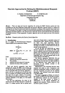
3. Solving Methods for OCSPs 3.1. S YSTEMATIC S EARCH M ETHODS 3.1.1. Branch and Bound All specific OCSP models can be solved by methods based on depth-first branch and bound, an optimization procedure for finite combinatorial optimization. In the following, we provide a detailed explanation of these methods specialized for the binary Max-CSP problem, an instance of the weighted model where all constraints are binary and all constraints have the same weight. A solution of the Max-CSP problem is an assignment satisfying as many constraints as possible. Many of the strategies developed below can be adapted to other models. Depth-first branch and bound (BnB) performs a depth-first traversal on the search tree defined by the problem, where internal nodes represent incomplete assignments and leaf nodes stand for complete ones. Assigned variables are called past (P), while unassigned variables are called future (F ). The distance of a node is the number of constraints violated by its assignment. At each node, BnB computes the upper bound (UB) as the distance of the best solution found so far, and the lower bound (LB) as an underestimation of the distance of any leaf node descendant from the current one. When UB LB, we know that the current best solution cannot be improved below the current node. In that case, the algorithm prunes all its successors and performs backtracking. The efficiency of BnB-based algorithms largely depends on the quality of the lower bound, which should be both as large and as cheap to compute as possible. At the current node, the simplest lower bound is the number of inconsistencies among past variables, LB(P) = distance(P) The BnB algorithm with this lower bound appears in Fig. 3.1.1. Procedure BB receives the following arguments: P is the set of past variables, F is the set of future variables, and FD is the collection of future domains. First, it checks if a leaf node has been reached (line 1). If so, it updates the best solution BestS (line 2) and the upper bound UB (line 3). Otherwise, it selects Xi as the current variable (line 5) and performs a loop checking every value of Xi (lines 6 to 9). If the lower bound computed with value a of Xi (line 10) reaches the upper bound, this branch is pruned. Otherwise, search continues along this branch (recursive call of line 8). It is assumed the existence of a function distance, which takes a set of assigned variables and returns the number of constraints among variables in the set unsatisfied by their current assignment.

paper.tex; 21/09/2001; 16:08; p.11

12


procedure BB(P; F; FD) 1 if (F =Ø) then 2 BestS assignment(P); 3 UB distance(BestS); 4 else 5 Xi select-variable(F ); 6 while FDi 6= Ødo 7 a select-value(FDi ); 8 if (LB(P; Xi ; a) < UB) then BB(P [fXi ; ag; F ?fXig; FD ?fFDi g) 9 FDi FDi ?fag; endprocedure function LB(P; F; Xi ; a; FD) 10 return distance(P [fXi ; ag);

Figure 1. Depth-first branch and bound algorithm.

3.1.2. Partial Forward Checking The partial forward checking (PFC) algorithm combines the branch and bound schema enhanced with forward checking lookahead (Freuder and Wallace, 1992) (in that paper this algorithm was called P-EFC3). PFC keeps for all feasible values of future variables the number of inconsistencies with previous assignments. The inconsistency count associated with value a of variable Xi, icia , is the number of inconsistencies that value a of Xi has with the assignments of past variables. The sum ∑ j2F minb (ic jb ) is a lower bound of the number of inconsistencies that will necessarily occur between variables of P and F if the current partial assignment is extended into a total one. This term can be added to the distance of past variables to compute the lower bound of the current partial assignment, because both terms record different inconsistencies. The new lower bound is, LB(P; F ) = distance(P) +

∑ minb(ic jb )

j2F

In addition, a value b of a future variable X j can be pruned if the lower bound, where the minimum contribution of X j is substituted by ic jb , is not lower than the upper bound. The PFC algorithm appears in Fig. 2. The main procedure presents three new lines with respect to the BB algorithm of Fig. 3.1.1, lines 9, 10 and 11. The lookahead function updates future domains (line 9). If no empty domains have been found and the new lower bound (possibly updated by the lookahead function) does not reach the upper bound (line 10), search continues along this branch (recursive call of line 11). The lookahead function considers all feasible future values (double loop in lines 13 and 14), checking if they can be pruned before (line 15) or after

paper.tex; 21/09/2001; 16:08; p.12


13

procedure PFC(P; F; FD) 1 if (F =Ø) then 2 BestS assignment(P); 3 UB distance(BestS); 4 else 5 Xi select-variable(F ); 6 while FDi 6= Ødo 7 a select-value(FDi ); 8 if (LB(P; F; Xi ; a; FD) < UB) then 9 NewFD look-ahead(P; F; Xi; a; FD; UB); 10 if (not empty_domain and LB(P; F; Xi ; a; NewFD) < UB) then 11 PFC(P + fXi ; ag; F ?fXig; NewFD) 12 FDi FDi ?fag; endprocedure function look-ahead(P; F; Xi; a; FD; UB) 13 forall j 2 F ?fXi g do 14 forall j 2 FD j do 15 if (LB jb (P; F; Xi ; a; FD) UB) then FD j FD j ?fbg 16 elseif (inconsistent(Xi; a; X j ; b)) then 17 ic jb ic jb + 1 FD j ?fbg 18 if (LB jb (P; F; Xi ; a; FD) >= UB) then FD j 19 return FD; function LB(P; F; Xi ; a; FD) 20 Newd distance(P) + icia; 21 return Newd + ∑ j2F; j6=i minb ic jb ; function LB jb (P; F; Xi ; a; FD) 22 Newd distance(P) + icia; 23 return Newd + ic jb + ∑k2F;k6=i; j minc ickc ;

Figure 2. Partial forward checking algorithm.

(line 18) updating their inconsistency counts (line 17). It returns the new set of future domains. Functions LB and LB jb compute, respectively, the lower bound at the current node and the lower bound for a future variable X j taking value b. Directed Arc-Inconsistency Counts. While distance of P records inconsistencies among past variables, and inconsistency counts record inconsistencies between past and future variables, directed arc-inconsistency counts record inconsistencies among future variables. Given that each term records violations of different constraints, they can be added (with some care) to form

paper.tex; 21/09/2001; 16:08; p.13

14


a new lower bound. Different versions of DAC have produced three different lower bounds for the PFC algorithm. In the following we present these versions in chronological order. Static DAC. Given a static variable ordering, the DAC associated to value a of variable Xi, dacia , is the number of variables which are arc-inconsistent with value a for Xi and appear after Xi in the ordering (Wallace, 1995). A variable is arc inconsistent with value a for Xi if all its values are incompatible with a. The counter dacia is a lower bound of the number of inconsistencies that Xiwill have with variables after Xi in the ordering if a is assigned to Xi . It is worth noting that each arc inconsistency is recorded in one DAC only, because they are directed. The sum ∑ j2F minb {dac jb } is a lower bound of the number of inconsistencies that will necessarily occur among variables of F if the current partial assignment is extended into a total one. This term can be added to the distance of past variables plus the sum of ICs, to compute the lower bound of the current partial assignment, because they record different inconsistencies. The new lower bound is (Wallace, 1995), LB(P; F ) = distance(P) +

∑ minb (ic jb ) + ∑ minb (dac jb )

j 2F

j2F

which can be substituted advantadgeously by (Larrosa and Meseguer, 1996), LB(P; F ) = distance(P) +

∑ minb (ic jb + dac jb )

j 2F

since icia + dacia is the minimum number of inconsistencies that will necessarily occur among pairs of non past variables if value a is assigned to Xi . With this lower bound, the PFC algorithm remains the same (now it is called PFC-DAC), changing the functions computing the lower bound, which are detailed in Fig. 3. Notice that in function LB jb, the dacia is not added to the result because these inconsistencies have been recorded as ICs on future variables by the function lookahead. Using static DAC, PFC must follow for variable instantiation the same ordering used in DAC computation. DACs are computed in a preprocessing step, before PFC starts. Inferred and Cascaded DAC. If values a, b with minimum DAC of two constrained variables Xi and X j , X j after Xi in the static ordering, are incompatible and dacia does not include an inconsistency from Ci j , dacia can be incremented in 1. In the best case values a, b will be selected for their variables, and they are incompatible. Otherwise, other values with higer DAC contribution will be selected. In both cases, the increment of dacia is justified. This approach is called inferrerd DAC (Wallace, 1996). If inferred DAC are used as before, we talk about cascaded DAC, which have to be computed with care, recording the contribution of each constraint to avoid adding twice the same inconsistency. When using cascaded DAC in lower bound computation, only contributions of variables not conected with the current one can be added

paper.tex; 21/09/2001; 16:08; p.14


15

function LB(P; F; Xi ; a; FD) 20 Newd distance(P) + icia; 21 return Newd + dacia + ∑ j2F; j6=i minb (ic jb + dac jb); function LB jb (P; F; Xi ; a; FD) 22 Newd distance(P) + icia; 23 return Newd + ic jb + dac jb + ∑k2F;k6=i; j minc (ickc + dackc );

Figure 3. Lower bound functions for static DAC.

(otherwise, duplications may occur). The author suggests to compute two lower bounds, one from static DAC and other from cascaded DAC, using the largest for pruning purposes. Reversible DAC. A new approach uses reversible DAC, relaxing the condition of a static variable ordering. Its only requirement is that constraints among future variables must be directed: if Ci j is a contraint between future variables, it is given a direction, for instance from j to i. Arc-inconsistencies of Ci j are recorded in the DAC of Xi . In this way, the same inconsistency cannot be recorded in the DAC of two different variables. Directed constraints among future variables induce a directed constraint graph GF , where Nodes(GF ) = F and Edges(GF )={( j,i) j Ci j between future variables, direction of Ci j from j to i}. Given a directed constraint graph GF , the graph-based DAC of value a of variable Xi , dacia (GF ), is the number of predecesors of Xi in GF which are arc-inconsistent with value a for Xi . The minimum number of inconsistencies recorded in variable X j , MNI(Xi,GF ), is as follows, MNI (X j ; GF ) = minb (ic jb + dac jb (GF )) and the graph-based lower bound (based onGF ) is, LB(P; F; GF ) = distance(P) +

∑ MNI(X j

j2F

;

GF )

With graph-based DAC any dynamic variable ordering can be used. This approach is complemented with the dynamic selection of GF . Given that any GF is suitable for DAC computation, a local optimization process looks for a good GF with respect to current IC values at each node. Since the only possible change in GF is reversing the orientation of its edges (by reversing the direction of its constraints), this approach is called reversible DAC. These features are included in the PFC-MRDAC algorithm (Larrosa et al., 1999), where in addition, DAC are updated during search considering future value pruning.

paper.tex; 21/09/2001; 16:08; p.15

16


The algorithm implementing these features appears in Fig. 4 and it is relatively complex for a detailed description. The differences with PFC (Fig. 2) start at line 10. If the current branch is not pruned, a better directed graph GF is searched by a greedy optimization method (line 11), and the test for pruning the current branch is repeated (line 12). If the search continues, future values are tested for pruning by function delete (line 13), where GF is specialized for each future value to maximize value removal. If no future domain becomes empty, DAC are maintained with respect to previous value removal in function prop-del, which again test future domains (line 15). If no empty domain is found, search continues along the current branch with the recursive call (line 17). Partition-Based LB. So far, the lower bound has recorded contributions of individual future variables. This approach (Larrosa and Meseguer, 1999) consider the partition P(F )={Fq } of the set F, and the lower bound is computed as the aggregation of contributions from each element of the partition. The minimum number of inconsistencies provided by a subset Fq = fXi ; : : : ; X p g is, MNI (Fq; GF ) = minb1

bp

;:::;

∑

j2Fq

F 0 [ic jb j + dac jb j (G )] + cost ((Xi ; bi ); : : : ; (X p ; b p ))

where value b j corresponds to variable X j . The expression cost’((Xi ,bi ), . . . ,(X p,b p )) accounts for the number of constraints among variables in Fq which are violated by the values {bi , . . . ,b p } and this violation is not recorded as directed arc inconsistency. The new lower bound, called partition-based because it depends on the selected partition, is defined, LB(P; P(F ); GF ) = distance(P) +

∑

F q2P(F )

MNI (Fq; GF )

A central aspect of this approach is finding easily good partitions. For efficiency reasons, authors restrict the search to partitions with subsets of up two elements, which are computed following a greedy approach. If merging two future variables into a partition element increases their contribution in 1 (the respective minimua of IC+DAC are incompatible, but this inconsistency is not recorded in any DAC), they are merged. In this way, the partition is computed, and the associated lower bound is obtained. It is easy to check that the partition-based lower bound is always higher than or equal to the reversible DAC lower bound. Arc-Inconsistency Counts The arc-inconsistency count (AC) associated to value a of variable Xi , acia , is the number of future variables which are arc-inconsistent with value a for Xi (Freuder and Wallace, 1992). A variable is arc inconsistent with value a for Xi if all its values are incompatible with a. Using AC

paper.tex; 21/09/2001; 16:08; p.16


17

procedure PFC-MRDAC(P; F; FD; GF ) 1 if (F =Ø) then 2 BestS assignment(P); 3 UB distance(BestS); 4 else 5 Xi select-variable(F ); 6 while FDi 6= Ødo 7 a select-value(FDi ); 8 if (LB(P; F; Xi ; a; FD; GF ) < UB) then 9 NewFD look_ahead(P; F; Xi; a; FD; UB; GF ); 10 if (not empty_domain) 11 NewFD greedy-opt(GF ; F; NewFD); 12 if (LB(P; F; Xi ; a; NewFD; NewGF ) < UB) then 13 NewFD delete(F; NewFD; NewGF ); 14 if (not empty_domain) 15 NewFD prop-del (F; NewFD); 16 if (not empty_domain) 17 PFC-MRDAC(P + fXi; ag; F ?fXi g; NewFD; NewGF ) 18 FDi FDi ?fag; endprocedure

Figure 4. PFC with maintaining reversible DAC.

instead of DAC for lower bound computation may cause to count twice an inconsistency (suppose that Ci j forbids all value pairs between Xi and X j ). A way to overcome this fact is to weight AC contributions with 1/2, in such a way that the contribution of an inconsistency cannot be counted twice. The lower bound proposed is (Affane and Bennaceur, 1998) LB(P; F ) = distance(P) +

∑ minb (ic jb + 1

j 2F

=

2ac jb )

This approach can be generalized to consider any weights such that wi j + w ji = 1, where is the weight that multiplies AC contributions of Ci j in variable Xi. Weights can also change dynamically during search. Determining how weights evolve is an open question of this method. Russian Doll Search The idea of Russian Doll Search (RDS) (Verfaillie et al., 1996) is to replace one search by n successive searches on nested subproblems. Given a static variable ordering, the first subproblem involves the last variable only, the ith subproblem involves all the variables from the n ? i + 1 to the last, and the nth subproblem involves all variables. Each subproblem is optimally solved using a PFC algorithm, following an increasing variable order: the first variable has the lowest number in the static ordering, and the last is always the n variable. The central point of this technique is that, when

paper.tex; 21/09/2001; 16:08; p.17

18


solving the whole problem, subproblem solutions obtained before can be used in the lower bound in the following form, LB(P; F ) = distance(P) +

∑ minb (ic jb ) + distance(Bestsolution(F ))

j2F

Let us suppose that we are solving the whole problem and P involves the first n ? i variables. The set F involves from n ? i + 1 to n variables, that is, F is composed by the variables of the ith subproblem. Then, the distance of the best solution found in that problem can be safely added to the contribution of P plus ICs to form the lower bound. This strategy is also used when solving the subproblem sequence. Solving subproblem i involves reusing all solutions from previously solved subproblems. 3.1.3. Systematic Search Heuristics As in CSP solving, heuristics for variable and value ordering are used. Regarding static variable ordering, required by PFC-DAC or RDS algorithms, the following heuristics have been reported. Decreasing backward degree (BD) (Wallace and Freuder, 1993). It considers first variables most constrained with past variables. It is expected that these variables will have high IC in their values, so after variable assignment the current distance is likely to increase. Its main disadvantage is the lack of information at the first levels of the tree. Decreasing forward degree (FD) (Larrosa and Meseguer, 1996). It considers first variables most constrained with future variables. This heuristic tries to increase the propagation of IC towards future variables, increasing the IC contribution to the lower bound. Decreasing degree (DG) (Wallace and Freuder, 1993). It can be seen as a combination of the two previous, BD and FD. At first levels of the tree FD dominates, while at deep levels BD dominates. Decreasing AC mean (AC) (Wallace and Freuder, 1993). It consider first variables with high AC. Variables with high AC will probably have also high DAC, so it tries to increase the DAC contribution to the lower bound. These heuristics and their combinations have been tested for PFC-DAC algorithms (Larrosa and Meseguer, 1996). Their conclusion on random problems is that the combination FD/BD (FD as first criterion, breaking ties with BD) is the most effective combination and, in addition, it is quite chip to compute. For the RDS algorithm, variable orderings with limited bandwith seem to be more adequate. Regarding dynamic variable ordering, required by PFC, PFC-RDAC or PFC-PRDAC algorithms, the classical heuristic of minimum domain (DOM) is preferred, selecting first the variable with the minimum number of values in its domain. Regarding PFC, (Wallace, 1996) provided a set of experiments

paper.tex; 21/09/2001; 16:08; p.18


19

on problems with low connectivity, concluding that combinations BD/AC and BD/DOM/AC were good choices. Considering PFC-RDAC and PRDAC, both use DOM divided by FD, a popular combination in classical CSPs. Regarding heuristics for dynamic value selection, in BnB-based algorithms most promising values (violating less constraints) are selected first. The goal it to decrease the upper bound, which will improve search efficiency. Therefore, in all described algorithms values are ordered by either (i) increasing IC, (ii) increasing IC+DAC, or (iii) increasing IC+AC. No comparative studies among the three criteria have been reported. 3.2. L OCAL S EARCH M ETHODS Greedy local search algorithms have been successfully applied to different classes of OCSP, mainly due to their efficiency. Local search algorithms start from an initial configuration and move from the current configuration to neighborhood configurations until a good solution is reached. These algorithms produce suboptimal solutions, since there is no guarantee for finding the optimal one. 3.2.1. Min-Conflicts Min-Conflicts (Minton et al., 1990; Minton et al., 1992) have been widely used to solve OCSP. Several versions of the Min-Conflicts procedures have been developed in recent years. They all differ from the basic ones in that they incorporate clever search techniques (Wallace and Freuder, 1995; Wallace, 1996). The Min-Conflicts algorithm chooses randomly any conflicting variable, i.e., the variable that is involved in any unsatisfied constraint, and then picks a value which minimizes the number of violated constraints. If no such value exists, it picks randomly one value that does not increase the number of violated constraints. Because the pure Min-Conflicts algorithm is unable to move beyond a local-minimum, the Min-Conflicts algorithm has been combined with the random-walk strategy. For a given conflicting variable, the random-walk strategy picks randomly a value with a probability p, and then apply the MinConflicts algorithm with a probability 1 ? p. The value of the parameter p has a big influence on the performance of the algorithm. Another version of the Min-Conflicts algorithm called the Steepest-Descent-Random-Walk has been proposed. This version explores the whole neighborhood of the current configuration and selects the best neighbour according to the evaluation value. One factor that limits the efficiency of local search algorithms is the size of the neighborhood. If there are many neighbors to consider, then the search will be very costly. To cope with this problem, Fast Local Search (FLS) has been introduced (Tsang et al., 1999). The main goal is, guided by heuristics, to ignore neighbours that are unlikely to lead to fruitful hill-climbs in order

paper.tex; 21/09/2001; 16:08; p.19

20


to improve the efficiency of a search. Each neighborhood move is associated with an activation bit. Only those neighbors whose bits are switched on will be considered in a hill-climbing step. All activation bits are switched on at the beginning. If a move has been examined in a hill-climbing step without leading to a better candidate solution, then its activation bit will be switched off. A connectionist approach called GENET (Davenport et al., 1994) has been proposed for solving CSP. In this approach, the problem is represented by a network with inhibitory links. GENET solves CSP by hill-climbing using a variation of the Min-Conflicts heuristic. GENET uses a constraint weighting scheme to escape local minima. When GENET encounters a local minimum, the weights of all the constraints which are violated in the minimum are increased. This increases the cost of violating constraints which are violated in the minimum, thus increasing the value of the cost function in the minimum and enabling the network to escape to other states. 3.2.2. Genetic Algorithms Genetic Algorithms (GA) (Goldberg, 1989) have been shown quite successful in a wide range of applications. GA borrow their ideas from evolution (Holland, 1975). The idea is to maintain a population of candidate solutions. The candidate solutions are given individual chances to produce offspring depending on their fitness. Fitness is measured by the objective function in optimization. GA have been applied to constraint satisfaction (Eiben et al., 1994; Ruttkay et al., 1995; Chu and Beasley, 1997). The use of GA in constrained optimization problems raises several issues to which a considerable amount of research has been devoted in the last years. One of the most important issues is how to incorporate constraints into the fitness function in order to guide the search properly. To incorporate constraints, one approach focussed on the use of penalty functions (Parmee, 1998). Several researchers have attempted to derive good techniques to build penalty functions. The work reported in (Homaifar et al., 1994) proposed a technique in which the user defines several levels of violations, and a penalty coefficient is chosen for each in such a way that the penalty coefficient increases as one reaches higher level of violations. 3.2.3. Simulated Annealing Simulated annealing (SA) (Kirkpatrick et al., 1983) is another stochastic search technique that has proved to be very effective for large scale optimization problems. In the SA technique, the temperature that is a variable is started at a high value and gradually reduces during the search. At high temperatures, moves are accepted in a random fashion regardless of whether they are uphill or down. As the temperature is lowered, the probability of accepting downhill moves drops and the probability of accepting uphill moves rises. A variant of

paper.tex; 21/09/2001; 16:08; p.20


21

SA (Li, 1997) has been applied to CSP’s that proved to be better than standard SA. This approach relies on dividing the search space into disjoints subspaces which are then processed by a localized SA strategy. Different temperatures and annealing speeds can be maintained in the different subspaces depending upon certain evaluation criteria. Another approach (Wah and Wang, 1999) combines SA with the theory of Lagrange multipliers, providing good results in discrete and continious problems. 3.2.4. Local Search Preprocess for Systematic Search To increase branch and bound efficiency, the lower bound should increase as fast as possible during search. In the same way, the upper bound should decrease as fast as possible, to enable the pruning condition, LB UB. In systematic search, most effort have been devoted to get large lower bounds, taking as starting upper bound the leftmost leave in the search tree. However, some local search can be done to get a better starting uper bound. In this sense, (Wallace, 1996), reported some experiments using three local search techniques to find an upper bound: (i) min-conflicts (Minton et al., 1992) with a random walk component, (ii) the breakout procedure (Morris, 1993), and (iii) weak commitment search (Yokoo, 1994). They were used as any time procedures, getting in the first seconds of execution, a quite significant improvement in the upper bound. In the same line, the decrement of the initial upper bound by mean field annealing (Cabon et al., 1996) causes visible improvements in branch and bound efficiency. 3.3. A PPROXIMATION M ETHODS Systematic search methods compute the optimal solution, but they are often too expensive when solving real problems. Local search methods compute suboptimal solutions, but they cannot determine how far they are from the optimal one. Approximation methods provide an alternative approach. Instead of looking for one solution, they look for an interval [lower bound, upper bound] enclosing the optimal solution. If the lower bound equals the upper bound, the optimum has been found. Otherwise, the distance between the upper and lower bounds can be used to assess the quality of the current solution. With this information, the user may decide when to stop the search, taking a suboptimal solution of reasonable quality. Approximation methods combine previous solving approaches. Solution candidades producing the upper bound can be easily computed by local search methods. Systematic search strategies can be adapted for anytime lower bound computation. Three different methods for anytime lower bounds are presented in (Cabon et al., 1998), Problem simplification: a lower bound is computed by solving completely a simplified problem. The optimum of the simplified problem either is a lower

paper.tex; 21/09/2001; 16:08; p.21

22


bound or allows such a bound to be computed. In (Givry et al., 1997), a simplification is produced by modifying the violation function. Objective simplification: a lower bound is computed by aiming at a simpler objective, like local consistency. For example, the sum of DAC at the root of the tree search (Larrosa et al., 1999), is a problem lower bound. More generally, the set of constraints which have to be removed to achieve any kind of classical local consistency property in the problem, can be used to compute a problem lower bound. Search simplification: the idea is performing a limited tree search and exploiting subproblem lower bounds in order to produce a problem lower bound. A number of algorithms has been explored in (Cabon et al., 1998). The combination iterative deepening + russian doll search produces the best results in both random and real benchmarks. It follows the russian doll approach, substituting one search by n nested searches of subproblems. However, each subproblem is not solved to optimality but a subproblem lower bound is computed using an iterative deepening algorithm. Interestingly, at the jth subproblem, the contribution of lookahead can be safely added with the lower bound of the j+1th subproblem, to compute a lower bound for the jth subproblem. The last subproblem is the whole problem, and then the problem lower bound is computed. 3.4. M ULTI -O BJECTIVE O PTIMIZATION In the following, we outline some methods to solve OCSPs when formulated as multi-objective optimization problems. For more details, the reader is addressed to specific bibliography (Rosenthal, 1985). The goal in multiobjective optimization is to construct the Pareto set E (P). Assuming that all the states in E (P) are of equal value, any can be taken as the problem solution. A good approach would be to generate a representative sampling of E (P), on which a decision support system could make a final choice. If this is too costly, the sampling is approximated. 3.4.1. Parametric Scalarization An approach to multi-objective optimization, F= ( f1 ,. . . ,f k);is to specify a weight vector, w=(w1 ,...,wk ), such that wi 0 and ∑ wi = 1. Each wi gives a weight to each objective function fi , representing our preferences among objectives. Given a suitable weight vector and an scalarizing function g: Rk > R, the multi-objective optimization problem ‘Minimize’ F(s) over all sg 2 S is substituted by the following single-objective optimization problem, Minimize g(F(s),w) over all sg 2 S Numerous researchers have discovered a connection between Pareto optimality and weights. Given suitable conditions on the objective functions and

paper.tex; 21/09/2001; 16:08; p.22

23


the state space we have that Pareto optimal points correspond to solutions of the optimization problem over the scalarizing function. Points on the Pareto frontier can be generated by solving the problem Pw for different weight vectors w, i.e. minimizing the aggregation function for different weight settings. Common functions are The weighted sum: The weighted sum is probably the most common scalarizing function. Sometimes it makes use of a fixed reference point z’, for instance an ideal point z* g(z,w) = ∑

wi zi org(z,w) = ∑

wi (zi ? z0i )

The Chebychev function: g(z,w) = maxi { wi (zi ? z0i ) } The l p -norm function: given p 1, g(z,w) = ( ∑ wi (zi ? z0i ) p ) 1 p Other scalarizing functions: g(z,w) = (1 - α) gc (z,w) + α/k gw (z,w) wheregc is the Chebychev function, andgw the weighted sum. We can now formulate a serie of single-objective optimization problem by varying these parameters, and solve them using traditional single-objective optimization methods. This will give us points on the Pareto set. =

3.4.2. Local Search As in the single-optimization case, local search is usually divided among a neighbourhood function tha generates successors from the current state, a selection function that determines which state will be selected as the next one, and meta-strategies to escape from local minima. These issues, hard enough in the single-objective case, become more difficult in multi-objective optimization. Selection among neighbours becomes more complicated because they may be non-comparable. Objective functions are usually scalarized, following the approaches mentioned in Section 3.4.1. When searching in the multi-objective case, we may find many states which are neither worse nor better than the “best” found so far, there is no dominance among them. A cache or archive is a way of collecting and handling non-dominant best states. This cache will contain, at any time, a subset of the best approximation found to the Pareto set. The criterion to include a new state in the cache is as follows. If the new state dominates any state in the cache, the dominated states are removed from the cache and the new state is added. If the new state is dominated by any other state of the cache, it is not added. If there is no dominance relation between the new state and any state of the cache, the new state is added to the cache. It belongs to the approximation of the Pareto set. Regarding SA procedures, the probability function is determined by using a probability scalarizing approach, where acceptance probabilities for each objective are aggregated. If pk is the acceptance probability for the

paper.tex; 21/09/2001; 16:08; p.23

24


k th objective function, the aggregated acceptance probability p is a function g( p1 ,...,pk ). A complete multi-objective Simulated Annealing algorithm (popularily called MOSA) was developed in (Ulungu et al., 1997). The MOSA algorithm has been improved and tested in (Ulungu et al., 1999). The paper illustrate the different options in the implementation of MOSA, and some typical behaviour of MOSA are explained by the possible complexity jump from solving uni-objective to multi-objective problems. The Mosa algorithm has been advocated for interactive use in an industrial setting (Ulungu et al., 1998). Regarding GA procedures, those states non-dominated by other states in the population are selected to move the population toward the Pareto set. These states are then assigned the highest rank and eliminated from further contention. Another set of Pareto non-dominated states are determined from the remaining population and are assigned the next high rank. This process continues until the population is suitably ranked. Finally, the rank of an individual determines its fitness value. Remarkable here is the fact that fitness is related to the whole population, while with aggregation techniques an individual’s raw fitness value is calculated independently of other individuals. Some popular algorithms are: Pareto ranking-based Genetic Algorithm (MOGA) (Belegundu et al., 1994), Non-dominated Sorting Genetic Algorithm (NSGA) (Srinivas and Deb., 1993), and Niched Pareto Genetic Algorithm (NPGA) (Horn and Nafplitis, 1993).

4. Solution Evaluation 4.1. C ASE S TUDIES 4.1.1. Earth Observation Satellite Management The problem consists on planing a daily management of a satellite to take a set of images from at least one of three instruments. The problem can be cast as a satisfaction plus optimization with binary, ternary an one n-ary constraint (Lemaitre and Verfaillie, 1997; Bensana et et al., 1999). Problem instances can be downloaded from ftp://ftp.cert.fr/pub/lemaitre/LVCSP/Pbs/SPOT5.tgz. Problem Formulation Variables: A variable is associated with each image. A positive integer weights each variable. Domain: It is formed by the possible assignment of the different instruments to take the image: three possible values for a mono image and only one value for a stereo image. Constraints: A set of hard binary constraints expresses the non overlapping and minimum transition time constraints. A set of hard binary or ternary constraints expresses the limitation of the instantaneous data flow through

paper.tex; 21/09/2001; 16:08; p.24


25

the satellite telemetry. An n-ary hard constraint involving all the variables expresses the limitation of the on-board recording capacity. Optimization criteria: The weight of a partial assignment is defined as the sum of the weigths of the assigned variables. A partial assignment is said feasible if and only if it satisfies all the hard constraints (with the n-ary constraint restricted to the assigned variables). The problem consists in finding a partial feasible assignment whose weight is maximum. Solving Methods and Results. Systematic methods are able to optimally solve problem instances without any n-ary recording capacity constraint. However, they fail to do so when this type of constraint is included. All the provenly optimal results have been obtained either using an ILP problem formalization and the CPLEX commercial software, or by using a Valued CSP formalization and Russian Doll Search. The original article of RDS (Verfaillie et al., 1996) implemented in LISP, reports very good results compared to Depth First Branch and Bound with backward and forward cheking on several instances, and notices the negative influence of increasing graph bandwith to the cpu solving time. The ILOG Solver has been experimented on smaller instances, and a comparison report exists (Lemaitre and Verfaillie, 1997). All the approximating results have been obtained with Tabu Search algorithms. In an operational context, an hour is currently considered as a maximum time to decide which images will be taken the next day and how to take them. Although this constraint cannot be considered as hard in the context of this benchmark it may be important that a program taking more than one day, would not be very useful.

4.1.2. TimeTabling This case study presents a possible overconstrained problem plus a multiobjective optimization problem (Schaerf, 1999). It includes constraints with high arity. The aim is to assign teachers to classes in a period of time in order to accomplish the requirement matrix and the teacher, and class availability matrices. Problem Formulation c1 ; :::; cm be m classes t1 ; :::; tn be n teachers 1,. . . ,p be p periods Rmnrequirements matrix: ri j is the number of lectures given by teacher t j to class ci Tm p tik is 1 if teacher ti is availale at period k, otherwise it is 0 Cn p cik is 1 if class ci is availale at period k, otherwise it is 0 Variables: find xi jk (i = 1::m; j = 1::n; k = 1:: p) Constraints:

paper.tex; 21/09/2001; 16:08; p.25

26


(1) xi jk = 0 or 1 (i = 1::m; j = 1::n; k = 1:: p) xi jk =1 if class ci and teacher t j meet at period k xi jk =0 otherwise (2) ∑kp=1 xi jk (i = 1::m; j = 1::n) right number of lectures to each class (3) ∑nj=1 xi jk tik (i = 1::m; k = 1:: p) each teacher is involved in at most 1 lecture for each period (4) ∑m i=1 xi jk c jk ( j = 1::n; k = 1:: p) each class is involved in at most 1 lecture for each period Preassignments can be added xi jk pi jk (i = 1::m; j = 1::n; k = 1:: p) where pi jk = 0 if there is no preassignment and pi jk = 1 when a lecture of teacher t j to class ci is preassigned to period k. Optimization problem To convert this into a optimization problem different objective functions are proposed: p n min ∑m i=1 ∑ j=1 ∑k=1 di jk xi jk a large di jk is assigned to periods k in which a lecture of teacher t j to a class ci is less desirable. Multicriteria objective: the didactic cost: spreading the lectures over the whole week the organizational cost: having a teacher available for possible temporary teaching posts. the personal cost: a specific day-off for each teacher. Introduce penalties for each soft constraint. The objective is to minimize the overall penalty. Other variants of the problem consider simultaneous lectures, teachers for more than one subject, uncovered classes, special rooms, etc. Solving Methods and Results.The problem is NP-complete. Without considering availability matrices, the problem is polynomial time solvable. Reductions to graph coloring (Neufeld and Tartar, 1974) have proven results on the existence of solution. Local search techniques have been applied for large amount of data like: tabu search (Costa, 1994; Alvarez et al., 1996; Schaerf, 1996), simulated annealing (Abramson, 1991), genetic algorithms (Colorino et al., 1992). Logic programming approaches (Kang and White, 1992) have shown advantatges on the expressivness of constraints. A constraint relaxation problem solver COASTOOL (Yoshikawa et al., 1996) has also been used, casting the problem as a Partial CSP. 4.1.3. The radio link frequency assignment problems The problem consists in assigning frequencies to a set of radio links defined between pairs of sites in order to avoid interferences. Each radio link is represented by a variable whose domain is the set of all frequences that are available for this link. All the constraints are binary, non linear, and have finite domains. All problem instances have been built from a unique real instance with 916 links and 5744 constraints, and include both feasible (a solution exists satisfing all the constraints) and unfeasible (a solution exists

paper.tex; 21/09/2001; 16:08; p.26


27

satisfing all hard constraints and minimizing the cost of violating some of the soft constraints) (Cabon et al., 1999). Instances can be downloaded from: ftp://ftp.cert.fr/pub/lemaitre/FullRLFAP.tgz, and from http://www-bia.inra.fr/T/schiex/Doc/CELARE.html. Problem Formulation Variables: The links iεX Domains: The finite set of frequencies available for each link Di Hard constraints: (1) For each link iεX a frequency fi has to be chosen from a finite set Di : fi εDi (2) Two links can define a duplex link j fi ? f j j = di j d stands for distance Soft constraints: (3) Some links may already have a pre-assigned frequency fi = pi . There is a mobility cost for violating this soft constraint specified by mi (4) Two links may interfere together j fi ? f j j > di j . There is a interference cost for violating this soft constraint specified by ci . Several problems can be defined: Feasibility: find an assignement of frequencies to each link such that all constraints are satisfied. NP-complete since by constraints (1) and (4) it is possible to express the k-coloring problem . Minimum span: minimize the largest frequency used in the assignement; it can be reduced to a short sequence of Feasibility problems using dichotomic search, and can simply be cast as Possibilistic/Fuzzy CSP by adding soft unary constraints on the domain values min maxi fi Minimum cardinality: minimize the number of different frequencies used in the assignement; more difficult than the min-span minj[i fi j Maximum feasibility: if all the constraints cannot be satisfied simultaneously, find the assignement that minimizes the sum of all the violation cost. It can be cast as Partial CSP min(∑ ci j violation(j fi ? f j j > di j ) + ∑ mi j violation( fi = pi )) Solving Methods and Results. Approximation techniques are applied to the large data sets to find good solutions without giving an optimality proof. The classical methods have been applied: local search including tabu search, simulated annealing, genetic algorithms, potential reduction. Some aproximations of local search techniques are very close to the optimum. For the calculation of lower bounds on the minimum number of used frequencies the following techniques are applied: Branch and cut: it can be applied in case that a linear programming (LP) formulation is used as a model. Then a branch and bound algorithm is applied that at every node of the search tree attempts to strengthen the LP bound of a LP relaxation version of the problem.

paper.tex; 21/09/2001; 16:08; p.27

28


Constraint satisfaction: Several specialized branch-and-bound algorithms have been applied. And lately algorithms for overconstrained instances proving optimality have been provided. Graph coloring techniques: Chromatic number aproximations on some modified version of the constraint graph gives good lower bound on the minimum number of used frequencies. (Lanfear, 1989) The systematic algorithms with best perfomance improve the lower bound of unsatisfied constraints between uninstantiated variables. In addition with usual techniques to calculate good upper bounds with heuristics and to take into account the inconsistencies between instantiated and uninstantiated variables. No comparative studies exists for these methods. They achieve good performances on proving optimallity on particular instances. Problems of type Maximum feasibility turn to be more difficult. Proving optimality appears to be considerably time-consuming, but results exists on nearly every instance. Only one instance can be considered as a decent benchmark for the feasability problem. (Cabon et al., 1998) show performances of combinations of Russian Doll Search with some iterative deeping techniques and they achieve good results on the calculation of anytime lower bound for the instances. 5. Summary and Perspectives In this paper we have given a short overview of the existing methods for modelling and solving OCSPs. The different models for OCSP formulation have been summarized, with special attention to the generic models on which several interesting properties on local consistency have been proved. Regarding solving methods, both systematic and local search families have been revised, devoting special attention to specific techniques to deal with overconstrained problems. Since some OCSP can be seen as multi-objective optimization problems, some notions on this topic have been presented. Finally, we have described three case studies to illustrate the usage of all previous techniques in real world problems. This field is currently in full development. The last years have lead to important developments in OCSP solving algorithms, and new advances can be expected in the next years. Among the promising directions for further research, we mention the improvement of lower bounds used in BnB-based algorithms, and the exploitation of the constraint graph topology to speed up search. A good example of the first direction is very interesting work on arc consistency for soft constraints (Schiex, 2000), where arc consistency is successfully redefined in the soft constraint context. This may cause better lower bounds to appear, as well as new redefinitions of other local consistency concepts. In the second direction, we mention the work on variable elimina-

paper.tex; 21/09/2001; 16:08; p.28


29

tion (Larrosa, 2000), which has been shown very effective when applied to OCSP. These positive results indicate that the solving capacity of existing technology will be substantially enhanced in the near future.

Acknowledgements This work was carried out inside the ECSPLAIN project (IST-99-11969). Authors thank the other members of the project for their support, as well as project reviewers for their constructive criticisms.

References Abramson (1991) Constructing School timetables using simulated annealing: sequential and parallel algorithms. Management Science 37(1):98-113, 1991. Affane M-S., Bennaceur H. (1998) A weight arc consistency technique for Max-CSP, Proc. of ECAI-98, 209-213, 1998. Alvarez-Valdes, Martin, G., Tamarit, J.M. (1996) Constructing Good Solutions for the Spanish School Timetabling problem. Journal of the Operational Research Society., 1996. Belegundu A.D. and Murthy D.V. and Salagame and Constant E.W. (1994) Multi-objective Optimization of Laminated Ceramic Composites Using Genetic algorithms, In Fifth AIAA/ USAF/ NASA Symposium on Multidisciplinary Analysis and Optimization, volume Paper 84-4363-CP, pages 1015- 1022, Panama City , Florida, 1994 . AIAA. Bensana E., Lemaitre M., Verfaillie G. (1999) Earth Observation Satellite Management, Constraints Vol4 Num 3, 1999. Bistarelli S., Montanari U., Rossi F. (1995) Constraint solving over semirings. Proc. IJCAI-95 Bistarelli S., Montanari U., Rossi F., Schiex T., Verfaille G., Fargier H. (1999) Semiringbased CSPs and Valued CSPs: Frameworks, Properties and Comparison. Constraints, 4, 199-240, 1999 Cabon B., De Givry S„ Lobjois L., Schiex T., Warners J. (1999) Radio Link Frequency Assignement, Constraints vol 4, Number 1, 1999 Cabon B., Verfaillie G., Martinez D., Bourret P. (1996) Using mean field methods for boosting backtrack search in constraint satisfaction problems. Proc of ECAI-96, 165-169, 1996 Cabon B., Givry S., Verfaillie G. (1998) Anytime lower bounds for constraint violation minimization problems, Proc. of CP-98. Chu, P., and Beasley, J.E. (1997) Genetic algorithms for the generalized assignment problem. Computers and Operations Research, Vol.24, pp:17-23, 1997. Colorni, Dorigo and Maniezzo (1992) A genetic algorithm, to solve the timetable problem. Technical report 90.060, Politecnico di Milano, Italy. Costa, D (1994). A Tabu Search Algorithm for Computing an Operational Timetable. European Journal of Operational Research 76:98-110. Davenport A., Tsang E., Wang C., Zhu K. (1994) GENET:A Connectionist architecture for solving constraint satisfaction problems by iterative improvement. Proc. of AAAI-94, 325330. Dubois D., Fargier H, Prade H. (1996) Possibility theory in constraint satisfaction problems: Handling priority, preference and uncertainty. Applied Intelligence 6, 287-309.

paper.tex; 21/09/2001; 16:08; p.29

30


Eiben, A.E., Raua, P-E., and Ruttkay, Zs. (1994) Solving constraint satisfaction problem using genetic algorithms. Proc., 1st IEEE Conference on Evolutionary Computing, pp: 543-547, 1994. Fargier H., Lang J. (1993) Uncertainty in constraint satisfaction problems: a probabilistic approach. Proc. ECSQARU-93, Lecture Notes Computer Science 747, 97-104. Fargier H. (1994) Problemes de satisfaction de constraintes flexibles:application a l’ordonnancement de production. Ph. D. Thesis, Univ. Paul Sabatier, Toulouse, France. Freuder E., Wallace R. (1992) Partial constraint satisfaction. Artificial Intelligence, 58, 21-71. Givry S., G.Verfaillie, T. Schiex (1997) Bounding the Optimum of Constraint Optimization Problems, Proc of CP-97. Goldberg, D.E. (1989), Genetic Algorithms in Search, Optimization and Machine Learning. Addition-Wesley Publishing Co., Reading, Massachusetts, 1989. Holland J. H. (1975) Adaptation in natural and artificial systems. University of Michigan press, Ann Arbor, MI. Homaifar A, Lai S. H.Y., and Qi, X. (1994), Constrained Optimization via Genetic Algorithms. Simulation 62(4):242-254. Horn J. and Nafpliotis N. (1993), Multi-objective Optimization using the Niched Pareto Genetic Algorithm, Technical Report Illi GA1 Report 93005, University of Illinois at urbana Champaign, Urbana, Illonois , USA, 1993. Kang, White (1992) A logic approach to the resolution of constraints in timetabling, European Journal of Operational Research 61: 306-317 Kirkpatrick, S., Gelat, C.,and Vicci, M. (1983) Optimization by simulated annealing. Science, Vol.220, No.4598, pages:671-80. Kumar V. (1992) Algorithms for constraint satisfaction problems: A survey. AI Magazine, spring 1992, 32-44. Lanfear (1989) Graph theory and radio link frequency assignment problems. Technical report, NATO, Allied Radio Frequency. Larrosa J. (2000). Boosting search with variable elimination. Proc. CP-00, 291-305. Larrosa J., Meseguer P. (1996) Exploiting the use of DAC in Max-CSP. Proc. of CP-96, 308322. Larrosa J., Meseguer P. (1999). Partition-Based Lower Bound for Max-CSP, Proc. of CP-99, 303-315. Larrosa J., Meseguer P., Schiex T. (1999) Maintaining reversible DAC for Max-CSP. Artificial Intelligence, 107(1), 149-163. Lemaitre M, Verfaillie G. (1997) Daily management of an earth observation satellite: comparairon of ILOG Solver with dedicated algorithms for Valued CSP, Proc. of the Third ILOG International Users Meeting, Paris, France. Li, Y. H. (1997) Directed Annealing Search In constraint Satisfaction and Optimization. PhD Thesis, Imperial College of Science, Department of Computing, 1997. Minton S., Johnson M., Philips A., Laird P. (1990) Solving large-scale constraint satisfaction and scheduling problems using a heuristic repair method. Proc. of AAAI-90, 17-24. Minton S., Johnson M., Philips A., Laird P. (1992) Minimizing conflicts: a heuristic repair method for constraint satisfaction and scheduling problems. Artificial Intelligence, 58:161205. Morris P. (1993) The breakout method for escaping from local minima. Proc. of AAAI-93, 40-45. Neufeld, Tartar (1974) Graph Coloring Conditions for the Existence of solutions to the timetable problem. Communications of the ACM 17(8) 450-453. Parmee I. (1989) The integration of evolutionary and adaptive computing technologies with Product/System design and realization. Springer-Verlag, Plymouth, United Kingdom, 1998.

paper.tex; 21/09/2001; 16:08; p.30


31

Rosenthal R. (1985) Principles of multiobjective optimization. Decision Sciences, vol 16, 133152, 1985. Ruttkay Zs, Eiben, A.E, and Raue, P.E (1995). Improving the performance of GAs on a GAhard CSP. Proceedings, CP95 Workshop on Studying and Solving Really Hard Problems, 157-171, 1995. Schaerf A. (1996) Tabu Search Techniques for large High-School Timetabling problems. Proc. of ECAI-96, 634-639, 1996. Schaerf A. (1999) A Survey of Automated Timetabling, Artificial Intelligence Review 13:87127, 1999. Schiex T., Verfaille G., Fargier H. (1995) Valued constraint satisfaction problems: Hard and easy problems. Proc. IJCAI-95 631-637, 1995. Schiex T. (2000) Arc consistency for soft constraints. Proc. CP-2000, xxx-xxx. Srinivas N. and K.Deb. (1993) Multi -objective Optimization using nondominated sorting in genetic algorithms, Technical report, Department of Mechanical Engeneering, Indian Institute of technology, Kanput, India, 1993. Tsang E. (1993) Foundations of Constraint Satisfaction. Academic Press, 1993. Tsang E., Wang C., Davenport A., Voudouris C., Lau T. (1999) A Family of Stochastic Methods For Constraint Satisfaction and Optimization. The first International Conference on The Practical Application of Constraint Technologies and Logic Programming, London, 1999. Ulungu, E.L., J. Teghem and Ph. Fortemps (1997) Heuristics for multi-objective combinatorial optimization by Simulated Annealing, in Gu, J., Chen, G., Wei, Q. and Wang, S. (eds), Multicriteria Analysis, Springer –Verlag, Berlin, 1997, pp. 269-278. Ulungu E.L., J. Teghem, P.H. Fortemps, D. Tuyttens (1999), MOSA method: a tool for solving multi-objective combinatorial optimization problems, Journal of Multi-Criteria Decision Analysis Volume: 8, Issue: 4, Date: July 1999, Pages: 221-236. Ulungu E.L., J. Teghem, and Ost, C.(1998) Interactive Simulate Annealing in a multi-objective framework: application to an industrial problem, J. Oper. Res. Soc., 49, 1044-1050, 1998. Verfaille G. Schiex T. (1994) Solution reuse in dynamic constraint satisfaction problems. Proc. of AAAI-94, 307- 312, 1994. Verfaillie G., Lemaitre M., Schiex T. (1996) Russian doll search for solving constraint satisfaction problems. Proc of AAAI-96, 181-187, 1996. Wah B., Wang T., (1999) Simulated annealing with asymptotic convergence for nonlinear constrained global optimization. Proc. of CP-99, 461-475, 1999. Wallace R. (1995) Directed Arc Consistency Preprocessing. Selected papers from the ECAI-94 Workshop on Constraint Processing, LNCS-923, M. Meyer editor, 121-137, 1995. Wallace R. (1996) Enhancements of branch and bound methods for the maximal constraint satisfaction problem. Proc. of AAAI-96, 188-195, 1996 Wallace R., Freuder E.C. (1993) Conjunctive width heuristics for maximal constraint satisfaction. Proc. of AAAI-93, 762-768, 1993. Wallace R., Freuder E.C. (1995) Heuristics Methods for Over-Constrained Constraint Satisfaction Problems. Proc. of CP-95, France, 1995. Wallace R., Freuder E.C. (1998) Stable Solutions for dynamic constraint satisfaction problems Proc. of CP-98, LNCS No. 1520, 447-461, 1998. Yokoo M. (1994) Weak-commitment search for solving constraint satisfaction problems. Proc. of AAAI-94, 313-318, 1994 Yoshikawa, Kaneko, Yamanouchi Watanabe. (1996) A Constraint-Based High School Scheduling System. IEEE 11(1) 63-72, 1996.

paper.tex; 21/09/2001; 16:08; p.31

paper.tex; 21/09/2001; 16:08; p.32

Current Approaches for Solving Over-Constrained Problems - CiteSeerX

Current Approaches for Solving Over-Constrained Problems - CiteSeerX

Suggest Documents

Committee Constructions for Solving Problems of ... - CiteSeerX

Heuristic Approaches for Solving the

Strategies for Solving Problems - People.fas.harvard.edu

Application of Operational Approaches to Solving ... - CiteSeerX

Evaluation of Approaches to Solving Electrocardiographic ... - CiteSeerX

Solving Examination Timetabling Problems using Honey ... - CiteSeerX

Solving Multiclass Classification Problems by Genetic - CiteSeerX

Solving Optimization Problems using the Matlab ... - CiteSeerX

Solving Mathematical Problems by Investigation - CiteSeerX

Solving Copper Corrosion Problems while Maintaining ... - CiteSeerX

Solving Employee Timetabling Problems by Generalized ... - CiteSeerX

Solving Two Supervisory Control Benchmark Problems ... - CiteSeerX

Solving Public Transit Scheduling Problems - CiteSeerX

Solving Cryptarithmetic Problems Using Parallel Genetic ... - CiteSeerX

Solving Dynamic Constraint Satisfaction Problems by ... - CiteSeerX

Solving challenging bioorganic problems by exciton ... - CiteSeerX

Solving Signal Decoupling Problems Through Self ... - CiteSeerX

Solving Various Weighted Matching Problems with ... - CiteSeerX

The Problems with Problem Solving - CiteSeerX

Solving Distributed Constraint Optimization Problems ... - CiteSeerX

Solving Dynamic Constraint Satisfaction Problems by ... - CiteSeerX

Solving Problems under Uncertainty Paradigm: Encoding ... - CiteSeerX

Solving Highly Constrained Search Problems with ... - CiteSeerX

Solving Algebra Problems Before Algebra Instruction - CiteSeerX