Available online at www.sciencedirect.com
ScienceDirect Procedia CIRP 10 (2013) 112 – 118
12th CIRP Conference on Computer Aided Tolerancing
Curvature-based registration and segmentation for multisensor coordinate metrology Haibin Zhaoa, Nabil Anwerb*, Pierre Bourdetb b
a Department of Mechanical Engineering, KU Leuven, Belgium LURPA-ENS Cachan, 61, Avenue du Président Wilson, 94235 Cachan, France
Abstract With the rapid development of multiple sensors for shape acquisition and inspection, point-based discrete shape modeling is being widely used in many engineering applications, e.g. reverse engineering, quality control, etc. Geometry processing, which aims at recovering information about topology, geometry and shape from the measured data is one of the critical issues to achieve multiple sensors integration in coordinate metrology. This paper presents a novel approach for discrete geometry processing in multisensor coordinate metrology. Two important issues are addressed here: registration and segmentation. We propose here a new modified Iterative Closest Point (ICP) algorithm to improve the registration performances by using the curvature information. Shape recognition and segmentation are the most critical issues of discrete geometry processing. The local surface types and the characteristic points are first recognized based on two surface descriptors: shape index and curvedness. A clustering method is developed to classify the vertices according to their surface types, and a connected region generation approach is developed for final segmentation. Finally, an industrial case study is presented to illustrate the entire approach, and to demonstrate the validity of the proposed methods for engineering applications. © 2013 The Authors. Published by Elsevier B.V. Open access under CC BY-NC-ND license. © 2012 The Authors. Published by Elsevier B.V. Selection and/or peer-review under responsibility of Professor Xiangqian Jiang. Selection and peer-review under responsibility of Professor Xiangqian (Jane) Jiang Keywords: multisensor; coordinate metrology; registration; segmentation; discrete curvatures
1. Introductiona With the rigorous and tightening requirements on measurement accuracy of complex shapes, multiple sensors are increasingly being employed in coordinate metrology. Multisensor integration and fusion process data of various sensors for holistic shape acquisition, while improving reliability and reducing measurement uncertainty [1]. With multisensor integration, shapes can be acquired by the most suitable combination of sensors. In general, the different sensors acquire the measurement information in different formats (image intensity, surface descriptors, volume data, etc.) at different resolutions and details. As a result, the following problems are
* Corresponding author. Tel.: +33-(0)147402413; fax: +33-(0)147402220. E-mail address:
[email protected].
arisen: How to fuse multisensor data for complete shape representation and how to derive the most interesting information from the acquired discrete shapes. Geometry processing, which aims at recovering information about topology, geometry and shape from the measured data is one of the critical issues to achieve multiple sensors integration in coordinate metrology. This paper presents a novel approach for discrete geometry processing in multisensor coordinate metrology. Two important issues are addressed here: shape registration and segmentation. Registration is one of the most important and decisive steps of multisensor integration [1]. The point data acquired by multiple views/sensors are usually represented in their own coordinate systems. Registration is used to transform the respective data into a common coordinate system and to obtain the complete model. The common used methods for data registration include marker based approaches [2], and ICP (Iterative
2212-8271 © 2013 The Authors. Published by Elsevier B.V. Open access under CC BY-NC-ND license. Selection and peer-review under responsibility of Professor Xiangqian (Jane) Jiang doi:10.1016/j.procir.2013.08.020
Haibin Zhao et al. / Procedia CIRP 10 (2013) 112 – 118
Closest Point) based algorithms [3]. Considerable ICP variants have been proposed in the literature, such as trimmed ICP [4], lookup matrix based ICP [5], etc. Shape recognition and segmentation are the most critical parts of discrete geometry processing [6-8]. The developed segmentation methods can be classified into three categories: edge-based, region-based and hybridbased. The edge-based methods [6] first detect the edges (or boundaries) of discrete models and the regions are then partitioned accordingly. Region-based methods [9], on the other hand, attempt to generate regions (points with similar properties) first. The boundaries are then computed from the regions. Edge-based methods are sensitive to the noise while region-based methods are a very time consuming problems [8]. The hybrid approaches [7, 10] combining the edge-based and region-based information have been emphasized in recent years to overcome the limitations of the two above approaches. According to the author’s knowledge, despite there have already been a large amount of works on registration and segmentation, key issues considering real shapes, noise and multiple resolutions have not been successfully solved yet. For registration, to improve convergence speed, invariant feature based ICP algorithms [11] have been developed. However, there is not a thorough investigation of registration from the perspective of invariant features based on curvatures. For segmentation, the problem to decompose the real noisy data has not been solved yet. Therefore, this paper proposes curvature based methods which focus on the registration and segmentation problems in engineering applications. The main contributions of this paper are twofold. First, we propose a new way to improve the ICP registration performance by using curvature information. The Euclidean distance and the curvature distance are combined together as a new measure of closest points. Our second contribution is to develop a new method to segment triangular mesh models for engineering applications. The proposed method is implemented to segment both tessellated CAD models and the measured data. The remainder of this paper is organized as follows. Section 2 describes the curvature-based registration method. Section 3 presents the segmentation method in details. In section 4, a real industrial case is studied to test the performances of the proposed methods and finally section 5 is the conclusion of this work. 2. Data registration Registration transforms the multiple data acquired from different sensors/views into a common coordinate system. In this section, we propose a new registration
method based on ICP algorithm. This method solves the registration problem of partial overlapping shapes with unknown correspondences. The proposed method is based on curvature information. Therefore, we first develop the methods needed to estimate discrete curvatures. 2.1. Discrete curvature estimation The raw data acquired directly from sensors are usually noisy, incomplete, redundant, etc. They should be preprocessed first to before discrete curvature estimation. Moreover, they also need to be approximated by proper watertight polyhedral surfaces in order to build the topology structures of shapes. Due to the linear smoothness of the input mesh, the discrete curvature estimation is subject to various definitions [12, 13]. We have implemented here the work of Cohen-Steiner and Morvan [12] based on the Normal Cycle. For each vertex, the curvature tensor is calculated and the principal curvature values and directions are computed as the eigenvalues and the eigenvectors of the curvature tensor. This estimation method is efficient and robust to provide reasonable results for noisy data. Moreover, The Cohen-Steiner and Morvan method can estimate the principal curvatures and the principal directions directly. These attributes are the basis of the computation of the shape index and the curvedness (see section 3.1) which are two important surface descriptors in our segmentation method. 2.2. Data registration The ICP algorithm [3] and its variants are the most popular methods for data registration. However, they usually require that the data be already aligned roughly in an initialization stage (coarse registration). In our case, we first search the corresponding features within the input point data, and then calculate the transformation between the detected features. Finally, we align the input data together. Because of the limited extent of the paper, the detailed coarse registration is omitted. More details can be found in [14]. After coarse registration, the general process of the ICP algorithm contains three procedures: (1) corresponding point pairs searching; (2) transformation matrix calculation and (3) alignment error computation and comparison. We propose a new modified ICP algorithm to improve the registration performances by using the curvature information. The new method also follows the three basic procedures as the classical ICP algorithm. The main contribution of the proposed method is that it defines a new distance called geometry distance to measure the closest point in corresponding
113
114
Haibin Zhao et al. / Procedia CIRP 10 (2013) 112 – 118
point pair searching. In this section, we denote the proposed method as CFR (Curvature-based Fine Registration). In registration process, the movable point data is denoted as scene data while the point data that is viewed as the reference is denoted as model data. Considering an arbitrary point in the scene data pi , and another arbitrary point q j in the model data, The geometry distance is defined as: d g ( pi , q j )
d e ( pi , q j ) (1
) d c ( pi , q j )
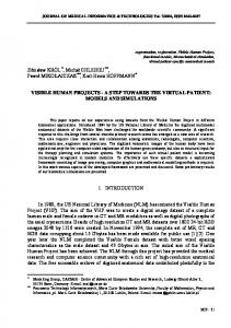
(a) (b) input data
(1)
(c) ICP method
(d) CFR method
Fig. 1: Registration results and comparison
Where,
d e ( pi , q j ) || pi
q j ||
is
the
Euclidean
distance between pi and q j . d c ( pi , q j ) is the curvature ratio distance between the two points, which has the following definition: d c ( pi , q j )
(
1 ( 1 pi )
1 2 ) ( 1 qj )
(
1 ( 2 pi )
1 2 ) (2) ( 2 qj )
are the 1 ( pi ) and 2 ( pi ) ( 1 ( q j ) and 2 (q j ) ) maximum and minimum principal curvatures of pi q j respectively. The curvature ratio distance and the Euclidean distance have the same length dimension. That’s the reason why we use curvature ratio distance as the way to integrate the curvature information in geometry distance definition. [0,1] is the weight to balance the contributions of d e ( pi , q j ) and d c ( pi , q j ) . The registration performance (see more details in [14]). depends on the values of Experimentally, if is set between [0.1, 0.8], the CFR method usually provides satisfying performances. In the corresponding point pairs searching stage, we apply the geometry distance instead of Euclidean distance to measure the closest point. For each scene point, the CFR searches its closest point in the model data. Because of the partial overlapping of the two input point data, the mismatched point pairs should be identified and rejected. In our method, we reject the point pairs which either has the larger geometry distances or the boundary point pairs. After rejection process, the reliable matched point pairs are used to calculate the geometric transformation between the two point data. Figure 1 gives an example of the registration results. The two input data (figure1. (a) (b)) contain 11831 and 10434 points respectively. The alignment error of the CFR method is 0.000848mm, taking 1644.25s with 13 iteration times (figure1. (d)) while the ICP algorithm takes 2911.78s with 40 iteration times and an alignment error of 0.01529mm (figure1. (c)).
3. Discrete shape recognition and segmentation We assume here that the initial discrete shapes are in the form of dense sets of points and can be broken down into various components, which meet along sharp or smooth edges. We also assume that the segmented components can be represented by lower order bivariate polynomials with degree no higher than three [9], which covers many engineering applications. With the above assumptions, our proposed method can always provide robust and accurate segmentation results. The method can be decomposed into three main phases: discrete shape recognition, vertex clustering and connected region generation.
3.1. Discrete curvature estimation The main indicators for surface type recognition in this paper are shape index and curvedness [15]. Shape index and curvedness are two shape indicators that specify the second order geometry of a shape. Shape index is a quantitative measure of the local surface type of a point on a surface. Mathematically, it is defined as a single value within [-1, 1] as in the following formula: s
2
arctan(
1
2
1
2
)
(3)
Curvedness, as a complementary parameter to the shape index, specifies the amount or intensity of the surface curvatures.
c
2 1
2 2
2
(4)
Where, 1 and 2 represent the maximum principal curvature and the minimum principal curvature respectively.
115
Haibin Zhao et al. / Procedia CIRP 10 (2013) 112 – 118
3.2. Surface type recognition
3.3. Vertex clustering
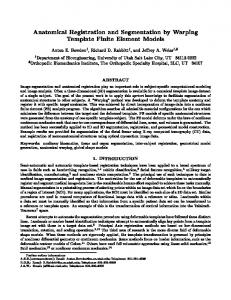
Koenderink and Doorn [15] defined nine basic surface types (figure 2) in a continuous way only using shape index. This definition is more convenient than the classical one based on Gaussian and Mean curvature. However, planar shapes are not defined based on the values of the shape index (here, we affect the planar shape a shape index equal to 2). The curvedness only vanishes on the ideal planar shape. Hence, a point can be identified as a planar point in practice if its curvedness value c ( p ) is less than a given threshold cth .
The vertices are first clustered into different categories. The vertices belonging to the same category have the similar characteristics. In our method, the vertices are first classified into ten categories according to their surface types. Due to measurement errors and computational errors (e.g. meshing error, curvature estimation error, etc.), the initial clustering results are far from being perfect. Therefore, we developed a cluster refining algorithm to improve the clustering performance. The cluster refining algorithm is based on an iterative process. Given a vertex, we firstly record all the surface types in its one-ring neighborhood. Then, we calculate the refining possibility of every surface type that the given vertex should be refined to. Finally, the surface type of the given vertex is refined into the category whose surface type has the maximum refining possibility. The iteration terminates when the surface type of each vertex doesn’t change or user-defined convergence condition occurs. Given a vertex vi , its surface type is labeled as T (vi ) , the set of the vertices in its neighbor region is denoted as N (vi ) . For an arbitrary vertex v j in N (vi ) , its surface type label is denoted as T (v j ) .
c( p)
(5)
cth
A set of color series is also assigned to represent the different surface types for visualization purpose [15]. A unique integer called surface type label is assigned to each of the ten surface types for convenience of the querying and processing [14]. The detailed specification of the ten defined surface types is highlighted in table 1.
Cluster distance between non-planar categories Here, we consider both T (vi ) and T (v j ) as nonplanar shapes. The cluster distance between two vertices vi and v j is then defined as: d c (vi , v j ) | T (vi ) T (v j ) | Fig. 2: 10 surface types defined by shape index and curvedness [14, 15]
(6)
Where, is a coefficient that defines the unit distance between two neighbor categories. Table 1: The specifications of the ten predefined surface types [14, 15] Surface type label
Surface type
Shape index interval
T=-4
Spherical cup
s
[ 1.0, 0.875]
T=-3
Through
s
( 0.875, 0.625]
T=-2
Rut
s
( 0.625, 0.375]
T=-1
Saddle rut
s
( 0.375, 0.125]
T=0
Saddle
s
( 0.125, 0.125]
T=1
Saddle ridge
s
(0.125, 0.375]
T=2
Ridge
s
(0.375, 0.625]
T=3
Dome
s
(0.625, 0.875]
T=4
Spherical cap
s
(0.875,1.0]
T=5
Plane
s
2
Cluster distance between planar and non-planar categories Considering the singularity of planar shapes, a planar vertex has the same possibility to be refined into any other non-planar categories. Therefore, the cluster distance is defined as: d c (vi , v j )
T (vi ) T (v j ) 5 T 1/ 9 (vi ) 5, T (v j ) 5 0
(7)
The cluster distance measures the similarity of local surface types between two vertices. Based on the cluster distance, the possibility to refine the vertex vi into the category T (v j ) is defined as follows:
116
Pvi [v j ]
Haibin Zhao et al. / Procedia CIRP 10 (2013) 112 – 118
[1 d c (vi , v j )] n j N ( vi )
([1 d c (vi , v j )] n j )
(8)
Where, n j denotes the number of the vertices whose surface type label is same as T (v j ) in N (vi ) . The possibility Pvi [v j ] gives a quantitative measure of the possibility and reliability to refine the vertex vi into the category T (v j ) . Finally, the vertex vi will be refined into the category whose surface type has the maximum refining possibility. After several iterations, the vertex clustering algorithm can provide reasonable results. 3.4. Connected region generation
Once the vertices are classified into different categories (vertices in the same category have the same surface type), we aim at recovering the connected regions and generate the final segmentation result. Two basic steps are considered here. Connected region growing which is performed to generate the initial segmentation result and region refining which aims to reduce the over-segmented regions and to improve the segmentation result. 3.4.1. Connected region growing The connected region growing method is based on the connected component labeling technique which is widely used in image processing [16]. When a vacant vertex that hasn’t been assigned with a region label is encountered, the vertex will be marked with a region label according to its neighbor condition. With this associated region label, the encountered vertex will either be integrated into an existing region or create a new region. The operation will terminate when there is no blank vertex at all within the given discrete model. The detailed growing mechanism is discussed below. vi is the encountered vacant vertex, its one-ring neighborhood is denoted as N (vi ) , The surface type label of vi is denoted as T (vi ) . Let, (vi ) represent the set of the vertices with surface type as T (vi ) in N (vi ) ; (vi ) denote the set of vertices whose surface type is different from T (vi ) in N (vi ) . When a vacant vertex is encountered, three neighbor conditions may occur, as shown in figure 3. The gray vertices represent the vertices in (vi ) .
(a) case 1
(b) case 2
(c) case 3
Fig. 3: Neighbor conditions for vacant vertex region labeling
Case 1 (figure 3 a): All the vertices in (vi ) haven’t been labeled yet. . In this case, a new region is created and a new region label (vi ) is associated with this region. The vertex vi and all the vertices in (vi ) are also associated with the new region label (vi ) . Case2 (figure 3 b): Some of the vertices in (vi ) have already been labeled with same region label (e.g. (v j ) ). In this case, the vertex vi and all other vacant vertices in (vi ) are associated with this region label (v j ) . Case 3 (figure 3 c): Some of the vertices in (vi ) have already been labelled, but with different region labels. In this case, if we denote the set of the different region labels as and (v j ) is the minimum value of , the vertex vi and all the vacant vertex in (vi ) are labelled with (v j ) . Moreover, the vertices whose region labels are in will be searched in the whole discrete model and relabelled as (v j ) . This operation aims to reduce the oversegmented regions during the region growing procedures. 3.4.2. Region refining The performance of the connected region growing depends on the vertex clustering results. The region refining is necessary to reduce the over-segmentation when the result of the connected region growing is not satisfying. Given a pair of adjacent regions R i , R j , we define a region distance to measure their similarity by the following formula: D( R i , R j )
dij pij nij
(9)
Where, d ij is a coefficient to measure the surface type similarity between the corresponding regions. pij is a coefficient considering the boundaries’ contribution for the region merging. The coefficient nij aims at eliminating the region compared to relative smaller
117
Haibin Zhao et al. / Procedia CIRP 10 (2013) 112 – 118
regions. The definitions of the three coefficients are more detailed in [14]. The region refining is performed as an iterative process. A priority queue of adjacent region pairs is generated according to their region distances. The adjacent regions pair with the maximum region distance are picked and merged into one region. The priority queue is then updated accordingly. Both the surface type and region label of the region with larger areas are assigned to the new generated region. The algorithm terminates when the number of the final regions or D( R i , R j ) reaches a predefined value. 4. Industrial case study
The algorithms mentioned in the previous sections have been implemented on a low-end PC platform (1.83 GHz CPU and 1G RAM) and considerable cases have been tested. The implementation is embedded in Microsoft Visual C++ supported by the CGAL libraries [17]. The visualization results are based on OpenGL libraries. 4.1. Data acquisition
A multisensor measurement system integrating three different sensors (Kreon Zephyr KZ25 laser scanner , a Renishaw TP2 probe and a STIL CHR150-CL2 chromatic confocal sensor) is used here (see Figure 4(a)). An automotive water pump cover is selected as a study case (Figure 4(b)). The pump cover has machined and rough surfaces. It should be an interesting case to test the performances of the proposed approaches for registration and segmentation. The workpiece is fully digitized using the multisensor platform. The data are acquired by laser scanning and touch probing in both complementary and competitive multisensor configurations. The global shape of the pump cover is captured by the laser scanner. The holes and the bottom plane are measured by the touch probe. Finally, 15 groups of scanned point data and 2 groups of probed point data are acquired.
(a) the multisensor platform
(b) the pump cover
Fig. 4: system setup for data acquisition
4.2. Registration
With the obtained 17 groups of point data, the registration process is performed based on an accumulative piecewise registration. Three examples of registration are shown in figure 5. The first example shows the registration of the point data acquired from different views (case 1)of the laser scanner (figure 5 (a)). The second example shows the registration of point data acquired from different poses (case 2) of the workpiece (figure 5 (b)). The last example shows the registration result when the two point data are acquired from different sensors (case 3) (figure 5 (c)). The alignment errors and time performance are shown in table 2. After registration, the complete model of the pump cover is generated. After filtering and denoising, the final complete model is shown in figure 6. It contains 141943 vertices. 4.3. Segmentation
Once the complete model is generated, the principal curvatures are estimated. The shape index and curvedness of the pump cover can then be computed for recognition and segmentation purpose. The final segmentation result of the pump is shown in figure 7 which proves that the result is satisfying for engineering applications. Table 2: Performances of studied cases in figure 5 case
Size of model data
Size of scene data
Align. error (mm)
1
30868
33550
0.0319
2
32838
21127
0.0408
3
17314
1200
0.0846
(a) different views
(b) different setups (c) different sensors
Fig. 5: Registration results of the pump cover
118
Haibin Zhao et al. / Procedia CIRP 10 (2013) 112 – 118
Fig. 6: The complete model of the pump cover
5. Conclusion
This paper presents new curvature-based registration and segmentation methods for coordinate metrology. In registration, we defined a new distance, named geometry distance, which combines the Euclidean distance and the curvature. A comparative analysis proves that the proposed method can provide better registration performances. In segmentation, the proposed method comprises three procedures: boundary identification, vertex clustering and connected region generation. The surface type definition based on shape index and curvedness provides a convenient way for shape recognition. The vertex clustering and connected region growing procedures reduce the noise influence. Finally, an industrial case study is presented to illustrate the entire approach, and to demonstrate the validity of the proposed methods for engineering applications. References [1] Weckenmann A., Jiang X., Sommer K., Neuschaefer-Rube U., Seewig J., Shaw L., Estler T. Multisensor data fusion in dimensional metrology. CIRP Annals- Manufacturing Technology 58, 2 (2009), 701–721. [2] Kim T.-W., Seo Y.-H., Lee S.-C., Yang Z., Chang M.: Simultaneous registration of multiple views with markers.Computer-Aided Design 41, 4 (2009), 231–239. [3] Besl P. J., Mckay N. D. A method for registration of 3-d shapes. IEEE Trans. on Pattern Analysis and Machine Intelligence 14, 2 (Feb. 1992), 239–256. [4] Chetverikov D., Svirko D., Stepanov D. The trimmed iterative closest point algorithm. Proc. of IEEE on ICPR’02 3 (2002), 545– 548.
Fig. 7: Segmentation results of the pump cover
[5] Almhdie A., Léger C., Deriche M., Lédée R. 3d registration using a new implementation of the icp algorithm based on a comprehensive lookup matrix: Application to medical imaging. Pattern Recognition letters 28, 12 (2007), 1523–1533 [6] Demarsin K., Vandersatraeten D., Volodine T., Roose D. Detection of closed sharp edges in point clouds using normal estimation and graph theory. Computer-Aided Design 39 (2007), 276–283. [7] Liu Y., Xiong Y. Automatic segmentation of unorganized noisy point clouds based on the gaussian map. Computer- Aided Design 40 (2008), 576–594. [8] Varady T., Martin R. R., Cox J. Reverse engineering of geometric models- an introduction. Computer-Aided Design 29, 4 (1997), 255–268. [9] Besl P. J., Jain R. C. Segmentation through variable order surface fitting. Trans. of IEEE on Pattern Analysis and Machine Intelligence 10, 2 (1988), 167–192 [10] Lavoue G., Dupont F., Baskurt A. A new cad mesh segmentation method, based on curvature tensor analysis. Computer-Aided Design 37, 10 (2005), 975–987. [11] Sharp G. G., Lee S. W., Wehe D. Icp registration using invariant features. Trans. on Pattern Analysis and Machine Intelligence 24, 1 (2002), 90–102. [12] Cohen-Steiner D., Morvan J.-M. Restricted Delaunay triangulation and normal cycle. In 19th Annual ACMSymposium on Computational Geometry’03 (2003), pp. 312–321. [13] Taubin G. Estimating the tensor of curvature of a surface from a polyhedral approximation. IEEE Proc. on Computer Vision and Pattern Recognition (1995), 902–907 [14] Zhao H. Multisensor integration and discrete geometry processing for coodinate metrology. Ph.D Thesis, Ecole Normale Superieure de Cachan, France (2010). [15] Koenderink J. J., Doorn A. J. Surface shape and curvature scales. Imaging and Vision Computing 10, 8 (1992), 557–565 [16] He L., Chao Y., Suzuki K., Wu K. Fast connected-component labeling. Pattern Recognition 42, 9 (2009), 1977–1987 [17] CGAL User and Reference Manual. CGAL Editorial Board, 3.9 edition. http //www.cgal.org/.