Curves in Calabi-Yau threefolds and Topological Quantum Field Theory

arXiv:math/0306316v2 [math.AG] 11 May 2004

Curves in Calabi-Yau threefolds and Topological Quantum Field Theory Jim Bryan and Rahul Pandharipande February 1, 2008 Abstract We continue our study of the local Gromov-Witten invariants of curves in Calabi-Yau threefolds. We define relative invariants for the local theory which give rise to a 1+1-dimensional TQFT taking values in the ring Q[[t]]. The associated Frobenius algebra over Q[[t]] is semisimple. Consequently, we obtain a structure result for the local invariants. As an easy consequence of our structure formula, we recover the closed formulas for the local invariants in case either the target genus or the degree equals 1.

1

Notation, definitions and results

A central problem in Gromov-Witten theory is to determine the structure of the Gromov-Witten invariants. Of special interest is the case where the target manifold is a Calabi-Yau threefold. We prove a structure result for the local Gromov-Witten invariants of a curve in a Calabi-Yau threefold. First, we define a relative version of the local invariants. In Theorem 1.2, we prove the new invariants determine a 1+1-dimensional semisimple TQFT taking values in the ring Q[[t]]. The structure formula for the invariants, Theorem 1.3, is obtained from the semisimple TQFT and completely determines the dependence of the invariants on the target genus. The local invariants are derived from considering rigid curves in CalabiYau threefolds. Let X be a non-singular curve of genus g in a Calabi-Yau threefold Y . Assuming certain rigidity conditions on X ⊂ Y , there are well defined local Gromov-Witten invariants of X in Y . That is, the contribution 1

2

1 NOTATION, DEFINITIONS AND RESULTS

to the Gromov-Witten invariants of Y by maps with image X is well defined. These local invariants depend only on g, h, and d, which are respectively, the target genus, the domain genus, and the degree of the maps to X. In [4], we defined an integral depending only on d, h, and g that gives the value of the local invariants whenever X ⊂ Y satisfies the requisite rigidity. The integral is given by Ndh−g (g) =

Z

[M h (X,d[X])]vir

c(I(X)),

see [4] (c.f. [3]) for details of this discussion. Here, c(·) denotes total Chern class and I(X) is defined by I(X) = −R• π∗ f ∗ (KX ⊕ OX ) = R1 π∗ f ∗ (KX ⊕ OX ) − R0 π∗ f ∗ (KX ⊕ OX ) which is understood to be an element of K-theory. It will be convenient to work with the version of the local invariants corresponding to stable maps with possibly disconnected domains: •

Definition 1.1. Let X be a non-singular curve of genus g. Let M (X, d) be the moduli space of degree d stable maps f :C→X where C is a possibly disconnected curve. We require f to be nonconstant on each connected component of C. Let •

•

[M (X, d)]vir ∈ A∗ (M (X, d); Q) denote the virtual fundamental cycle of the moduli space. Following [22], the superscript • is used to denote the moduli space with possibly disconnected domain curves. The usual genus subscript is omitted as we consider all domain genera: the moduli space is a countable union of connected components with varying expected dimensions. The branch points of a stable map to X are well-defined by [10]. The number of branch points b of map f equals the expected dimension of the moduli space at the moduli point [f ].

3


We define the (possibly disconnected) local Gromov-Witten invariants to be Z cb (I(X)). Zdb (g) = • [M (X,d)]vir

The relationship between the possibly disconnected invariants and the (connected) invariants Ndh−g (g) is easily seen to be XX

d>0 b≥0

where



Zdb (g)tbq d = exp 

XX

d>0 b≥0



Ndh−g (g)tb q d 

2h − 2 = (2g − 2)d + b. The generating function for the degree d, local, disconnected invariants is Zd (g) =

∞ X

Zdb (g)tb .

b=0

The series Zd (g) is our basic object of study. Clearly, the disconnected invariants Zdb (g) and the connected invariants Ndh−g (g) contain equivalent information. In Section 3, we use J. Li’s theory of relative stable maps [18, 19] to construct relative versions of the local invariants. These relative invariants obey a gluing law which allows us to construct a Topological Quantum Field Theory (TQFT): Theorem 1.2. There exists a 1 + 1-dimensional TQFT, Zd (−), with the following three properties: (i) Zd (−) is semisimple, (ii) Zd (−) takes values in Q[[t]], (iii) Zd (−) applied to a genus g closed surface yields the value Zd (g), the generating series of the local invariants. The t = 0 specialization of Zd (−) is a well-known TQFT obtained from the gauge theory of the symmetric group Sd , see Lemma 4.3. The TQFT determined by Sd was studied by Dijkgraaf-Witten and Freed-Quinn [6, 11]. Our TQFT may be viewed as a 1-parameter deformation of the DijkgraafWitten/Freed-Quinn theory.


4

Corresponding to any 1+1-dimensional TQFT is a Frobenius algebra. In our case, the dimension of the corresponding Frobenius algebra is p(d), the number of partitions of d. As a corollary of Theorem 1.2, we deduce the following structure formula. Theorem 1.3. There exist universal power series λα ∈ Q[[t]], labelled by partitions α of d (denoted α ⊢ d), which determine the local invariants by: Zd (g) =

X

λg−1 α .

α⊢d

Moreover, the constant term of the series λα is given by d! dim Rα

!2

where Rα is the irreducible representation of the symmetric group associated to α. The two main theorems of [23] (theorems 1 and 2) compute the local invariants in the case of degree 1 and the case of target genus 1. We recover these two results as immediate corollaries of the above structure theorem (Corollaries 1.5 and 1.4 below): Corollary 1.4. The series Zd (1) is the constant series p(d). In particular, the genus two and higher multiple cover contributions of a super-rigid elliptic curve are all zero. By the localization calculation of Faber-Pandharipande [9], Zd (0) is given by Zd (0) =

ℓ(α) αi t −2 t2d Y 2 sin( ) 2 α⊢d z(α) i=1 X

where the sum is over all partitions α of d. Here, ℓ(α) is the length of the α, and z(α) is a combinatorial factor (see Definition 3.3). In particular, for d = 1, we have !−2 sin(t/2) Z1 (0) = t/2 which we combine with our structure formula to deduce the following:

5

2 SEMISIMPLE TQFTS OVER COMPLETE LOCAL RINGS Corollary 1.5. The d = 1 local invariants are given by Z1 (g) =

sin(t/2) t/2

!2g−2

.

Recent progress (to be explained in a forthcoming paper [2]) has allowed us to completely determine the TQFT Zd (−) for small values of d. In particular, for d = 2 we have Theorem 1.6 ([2]). The d = 2 local invariants are given by Z2 (g) =

sin(t/2) t/2

!4g−4

n

o

(4 − 4 sin(t/2))g−1 + (4 + 4 sin(t/2))g−1 .

The above formula gives the double cover contributions of any smooth curve in a Calabi-Yau threefold with a generic normal bundle. The above formula also verifies the local Gopakumar-Vafa conjecture for degree 2 maps, i.e. the corresponding BPS invariants are integers. See [4] for a discussion of the BPS invariants and the local Gopakumar-Vafa conjecture.

2

Semisimple TQFTs over complete local rings

Let (n + 1)Cob be the symmetric monoidal category with objects given by compact oriented n-manifolds and morphisms given by (diffeomorphism classes of) oriented cobordisms. An (n + 1)-dimensional TQFT with values in a commutative ring R is a symmetric monoidal functor Z : (n + 1)Cob → Rmod, where Rmod is the category of R-modules. The definition amounts to the following axioms for Z: (i) To each compact oriented n-manifold Y , Z assigns an R-module Z(Y ). (ii) To each oriented cobordism W from Y1 to Y2 , Z assigns an R-module homomorphism Z(W ) : Z(Y1 ) → Z(Y2 ). (iii) If two oriented cobordisms are equivalent W ∼ = W ′ by a boundary preserving diffeomorphism, then Z(W ) = Z(W ′ ).

2 SEMISIMPLE TQFTS OVER COMPLETE LOCAL RINGS

6

(iv) The trivial oriented cobordism corresponds to the identity homomorphism, Z(Y × [0, 1]) = IdZ(Y ) . (v) The concatenation of cobordisms corresponds to the composition of the corresponding R-module homomorphisms. (vi) The disjoint union of n-manifolds corresponds to the tensor product ` of R-modules, Z(Y1 Y2 ) = Z(Y1 ) ⊗ Z(Y2 ), and the disjoint union of cobordisms corresponds to the tensor product of homomorphisms, ` Z(W1 W2 ) = Z(W1 ) ⊗ Z(W2 ).

(vii) The empty n-manifold corresponds to the ground ring, Z(∅) = R.

A compact oriented (n + 1)-manifold W may be viewed as a oriented cobordism between empty manifolds. Then, Z(W ) ∈ HomR (R, R) ∼ = R. The element Z(W ) ∈ R is a topological invariant of W . TQFTs of dimension 1+1 are in bijective correspondence with commutative Frobenius algebras. The result goes back to Dijkgraaf’s thesis, and has been proven in various contexts by Sawin [25], Abrams [1], and Quinn [24]. The form of the correspondence that we quote is due to Kock [16]: Theorem 2.1. The category of 1+1-dimensional TQFTs taking values in R is equivalent to the category of commutative Frobenius algebras over R. A commutative Frobenius algebra over R is a commutative Ralgebra A equipped with a counit µ : A → R and a coassociative, cocommutative, comultiplication △ : A → A ⊗ A satisfying the Frobenius relation and the counit axiom: (m ⊗ Id)(a ⊗ △(b)) = (Id ⊗ m)(△(a) ⊗ b) = △(m(a ⊗ b)) (Id ⊗ µ)(△(a)) = (µ ⊗ Id)(△(a)) = a where m : A ⊗ A → A is multiplication. The axioms imply that A is finitely generated as an R-module. Given an invertible element λ ∈ R, we can give R the structure of a Frobenius algebra by setting △(1) = λ and (consequently) µ(1) = λ−1 . We denote this Frobenius algebra by Rλ . A Frobenius algebra is semisimple if it is isomorphic to Rλ1 ⊕ · · · ⊕ Rλn for some λ1 , . . . , λn ∈ R.

2 SEMISIMPLE TQFTS OVER COMPLETE LOCAL RINGS

7

A 1+1-dimensional TQFT is semisimple if the corresponding Frobenius algebra is semisimple. If Wg is a closed surface of genus g, and Z is a semisimple TQFT, then an elementary argument from the axioms yields: Z(Wg ) =

n X

λg−1 . i

(1)

i=1

The following basic result is the key to proving the semisimplicity of the TQFT that we construct from local Gromov-Witten invariants. Proposition 2.2. Let R be a complete local ring. Let m ⊂ R be the maximal ideal and let A be a Frobenius algebra over R. Suppose that A is free as an Rmodule and that A/mA is a semi-simple Frobenius algebra over R/m. Then A is semi-simple (over R). Proof: Let e1 , . . . , en ∈ A be representatives for an idempotent basis of A/mA, that is ei ei − ei ∈ m for all i and ei ej ∈ m for all i 6= j. By Nakayama’s lemma, {ei } is a basis of A, and we wish to construct a new basis which is idempotent in A. We begin by constructing an idempotent basis in A/m2 A. It is easy to see that an element is invertible in A if and only if it is invertible in A/m. In particular, 1 − 2ei is invertible since its square is 1 modulo m. Let bi = ei ei − ei and set e′i = ei + bi (1 − 2ei )−1 . A short computation shows that e′i e′i − e′i = b2i (1 − 2ei )−2 which is in m2 for all i since bi ∈ m. Then e′i e′j ∈ m2 for i 6= j follows from the facts that (e′i e′j )2 , e′i e′i (e′j e′j − e′j ), and e′j (e′i e′i − e′i ) are all in m2 . Thus {e′i } is an idempotent basis for A/m2 . (k) We construct a sequence of bases {e′i }, {e′′i }, . . . , {ei } by setting (k)

bi

(k+1)

ei

(k) (k)

(k)

= ei ei − ei (k)

(k)

(k)

= ei + bi (1 − 2ei )−1 . (k)

The same argument as above shows that {ei } is an idempotent basis for (k) A/mk+1 A. Since R is complete, there exists e˜i ∈ A such that e˜i = ei mod

3 RELATIVE LOCAL INVARIANTS AND GLUING

8

mk+1 for all k. By construction, e˜i is an idempotent basis for A. Let λi = µ(˜ ei )−1 . Since A is free as an R-module, each e˜i generates an R summand of A and thus we have constructed the desired isomorphism of Frobenius algebras: A∼ = Rλ1 ⊕ · · · ⊕ Rλn .

3

Relative local invariants and gluing

Motivated by the symplectic theory of A.-M. Li and Y. Ruan [17], J. Li has developed an algebraic theory of relative stable maps to a pair (X, B). This theory compactifies the moduli space of maps to X with prescribed ramification over a non-singular divisor B ⊂ X, [18, 19]. Li constructs a moduli stack of relative stable maps together with a virtual fundamental cycle and proves a gluing formula. Consider a degeneration of X to X1 ∪B X2 , the union of X1 and X2 along a smooth divisor B. The gluing formula expresses the virtual fundamental cycle of the usual stable map moduli space of X in terms of virtual cycles for relative stable maps of (X1 , B) and (X2 , B). The theory of relative stable maps has also been pursued in [13, 14], [7]. In our case, the target is a non-singular curve X of genus g, and the divisor B is a collection of points b1 , . . . , br ∈ X. Definition 3.1. Let (X, b1 , . . . br ) be a fixed non-singular genus g curve with r distinct marked points. Let α1 , . . . , αr be partitions of d. Let •

M (X, (α1 . . . αr )) be the moduli stack of relative stable maps (in the sense of Li)1 with target (X, b1 , . . . , br ) satisfying the following: (i) The maps have degree d. (ii) The maps are ramified over bi with ramification type αi . (iii) The domain curves are possibly disconnected, but the map is not degree 0 on any connected component. (iv) The domain curves are not marked. 1

For a formal definition of relative stable maps, we refer to [18] Section 4.

9


The partition αi ⊢ d determines a ramification type over bi by requiring the monodromy of the cover (considered as a conjugacy class of Sd ) has cycle type αi . We will use a multi-index α = (α1 , . . . , αr ) to shorten the notation • to M (X, α) when there is no risk of confusion. Our moduli spaces of relative stable maps differ from Li’s in a few minor ways: (i) We do not require the domain to be connected. •

(ii) We do not fix the domain genus, so M (X, α) is a countable union of components. (iii) We do not mark the domain curve at all. Li’s spaces include a marking of the ramification locus. We make these modifications to Li’s theory to simplify the combinatorics of the gluing theory. It is straightforward to express our moduli spaces in terms of unions, products, and finite quotients of Li’s spaces. There is a universal diagram (of stacks): R⊂

-

U π

•

f

-

X

⊃

B

p

?

M (X, α) where U is the universal domain curve, X is the universal target curve, f is the universal map, B is the universal prescribed branch divisor, and R is the universal prescribed ramification divisor. The divisors B and R are taken with reduced structure. Note that the map f can also be ramified away from R, but at R the map f has the ramification type prescribed by the data α. One of the salient features of the relative theory is that the target curve may “bubble” off rational components meeting the original X in nodes. That is to say, the family • p : X → M (X, α) is nontrivial: special fibers have chains of rational curves attached to X at the points bi . However, the universal prescribed branch locus B lies in the non-singular locus of the fibers of p.


10

•

Let [M (X, α)]vir denote the virtual fundamental class. With our conventions, the virtual class is a countable sum of cycle classes with degree b part supported on the components of expected dimension b. The expected dimension of a component is given by b = −χ + ℓ(α) − d(2g − 2 + r) where ℓ(α) = ℓ(α1 ) + · · · + ℓ(αr ) is the sum of the lengths of the partitions and χ is the domain Euler characteristic. Let ω be the relative dualizing sheaf of p. We define an element I(X, α) • of the K-theory of coherent sheaves on M (X, α) by I(X, α) = −R• π∗ (f ∗ (ω(B)) ⊕ O(−R)) = R1 π∗ (f ∗ (ω(B)) ⊕ O(−R)) − R0 π∗ (f ∗ (ω(B)) ⊕ O(−R)). We define the relative local invariants by Zdb (g)α =

Z

•

[M (X,α)]vir

cb (I(X, α))

and their corresponding generating series Zd (g)α ∈ Q[[t]] by Zd (g)α =

∞ X

Zdb (g)α tb .

b=0

The element I(X, α) has rank b when restricted to the components of the • moduli space M (X, α) with expected dimension b. We regard I(X, α) as a (virtual) obstruction bundle and cb (I(X, α)) as the associated Euler class. Remark 3.2. In case g = 0 and r = 1, the above Euler class was previously defined by J. Li and Y. Song [20]. Li and Song were modeling “open string” Gromov-Witten theory using relative stable maps. They argued that the integral Zdb (0)α should compute the multiple cover formula for maps to a disk in a Calabi-Yau threefold where the boundary of the disk lies on a fixed Lagrangian 3-manifold (see also Katz-Liu [15]). They arrived at the integrand by considering the obstruction theory of maps to the disk with the Lagrangian boundary conditions. It is plausible that such an open-string theory interpretation of the relative local invariants exists in general. We will use Li’s theory to obtain “gluing relations” among the relative (and usual) local invariants. The following combinatorial quantity arises frequently:

11

4 THE TQFT

Definition 3.3. Let γ ⊢ d be a partition of d and let γ(k) be the number of P parts of size k in γ, so d = ∞ k=1 γ(k)k. We define: z(γ) =

∞ Y

k γ(k) γ(k)!.

k=1

If c(γ) ⊂ Sd denotes the conjugacy class in the symmetric group consisting of elements having cycle type γ, then z(γ) is the order of the centralizer of c(γ). The basic gluing laws are given by the following: Theorem 3.4. Let α = (α1 , . . . , αr ). For any choice g1 + g2 = g and any splitting {α1 , . . . , αr } = {α1 , . . . , αk } ∪ {αk+1, . . . , αr }, we have: Zd (g)α =

X

z(γ)Zd (g1 )α1 ,...,αk ,γ Zd (g2 )αk+1 ,...,αr ,γ .

(2)

γ⊢d

We also have Zd (g + 1)α =

X

z(γ)Zd (g)α1 ,...,αr ,γ,γ .

(3)

γ⊢d

The first formula corresponds to splitting a genus g surface with r boundaries along a separating curve to obtain two surfaces of genus g1 and g2 with (k + 1) and (r − k + 1) boundaries. The second formula corresponds to cutting a genus g + 1 surface with r boundaries along a non-separating curve to obtain a genus g surface with (r + 2) boundaries. We defer the proofs of these formulas to Appendix A.

4

The TQFT

We will show the gluing formulas of Theorem 3.4 allow us to organize the invariants Zd (g)α into a 1+1-dimensional TQFT over Q[[t]]. Throughout Section 4, R will denote the ring of formal power series in t over Q: R = Q[[t]].

12

4 THE TQFT

To define our TQFT, Zd (−), we need an R-module H = Zd (S 1 ) associated to the circle (H is the “Hilbert space” of the theory). We define Zd (S 1 ) = H =

M

R eα

α⊢d

to be a free R-module with a basis {eα }α⊢d labeled by partitions of d. Using the given basis for H, we can express any module homomorphism f : H ⊗r → H ⊗s ...βs in tensor notation fαβ11...α ∈ R by r

f (eα1 ⊗ · · · ⊗ eαr ) =

X

...βs fαβ11...α eβ1 ⊗ · · · ⊗ eβs . r

β1 ,...,βs

Using multi-index notation and the Einstein summation convention, we simply write: f : eα 7→ fαβeβ We raise indices by the following formula: s Zd (g)βα11,...,β ,...,αr = z(β1 ) · · · z(βs )Zd (g)α1 ,...,αr ,β1 ,...,βs .

Then the gluing laws can be written succinctly: δ β,γ Zd (g1 + g2 )β,δ α,η = Zd (g1 )α Zd (g2 )η,γ

Zd (g + 1)βα = Zd (g)β,γ α,γ Note that in the above equation, γ it is a single index, while the boldface indices (α, β, etc) stand for multi-indices. Since the γ is repeated on the left hand side, it is summed over by convention. Let Wrs (g) be the connected, oriented, genus g, cobordism from a disjoint union of r boundary circles to s boundary circles. We define Zd (Wrs (g)) : H ⊗r → H ⊗s by eα 7→ Zd (g)βαeβ where α = α1 , . . . , αr and β = β1 , . . . , βs . For a disconnected cobordism W = W1 ⊔ · · · ⊔ Wn , we define Zd (W ) = Zd (W1 ) ⊗ · · · ⊗ Zd (Wn ).

13

4 THE TQFT

Proposition 4.1. The functor Zd (−) defined above is a (1 + 1)-dimensional TQFT over R. Proof: To show Zd (−) is indeed a functor, we must prove that Zd (−) takes the concatenation of cobordisms to the composition of R-module homomorphisms. The composition Zd (Wst (g2 )) ◦ Zd (Wrs (g1 )) : H ⊗r → H ⊗s → H ⊗t determined by connected cobordisms is given by eα 7→ Zd (g1 )βαeβ 7→ Zd (g1 )βαZd (g2 )γβ eγ for α = (α1 , . . . , αr ), β = (β1 , . . . , βs ), γ = (γ1 , . . . , γt). Applying the gluing laws we obtain β1 ...βs 2 ...βs Zd (g1 )α Zd (g2 )γβ1 ...βs = Zd (g1 + g2 )γβ αβ2 ...βs 3 ...βs = Zd (g1 + g2 + 1)γβ αβ3 ...βs .. . = Zd (g1 + g2 + s − 1)γα .

(4)

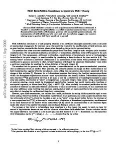
We have proven Zd (Wst (g2 )) ◦ Zd (Wrs (g1 )) = Zd (Wrt (g1 + g2 + s − 1)). Since the concatenation of Wrs (g1 ) followed by Wst (g2 ) is Wrt (g1 + g2 + s − 1) (see the Figure), we have shown that Zd (−) is a functor, at least when applied to the subcategory of 2Cob consisting of connected cobordisms. Similar computations apply to concatenations of disconnected cobordisms. For example, the concatenation of the cobordism Wr1 (g1 ) ⊔ Ws1 (g2 ) followed t by W2t (g3 ) yields the cobordism Wr+s (g1 + g2 + g3 ). Correspondingly, for α = (α1 , . . . , αr ), β = (β1 , . . . , βs ), δ = (δ1 , . . . , δt ), the composition Zd (W2t (g3 )) ◦ Zd (Wr1 (g1 ) ⊔ Ws1 (g2 ))

14

4 THE TQFT β1

α1

γ1

g2 g1 αr

γt

βs

Figure 1: Wrs (g1 ) concatenated with Wst (g2 ) is Wrt (g1 +g2 +s−1). The gluing formula expressed by this picture is given by Equation (4). is given by eα ⊗ eβ 7→ Zd (g1 )γα1 Zd (g2 )γβ2 eγ1 ⊗ eγ2 7→ Zd (g1 )γα1 Zd (g2 )γβ2 Zd (g3 )δγ1 γ2 eδ = Zd (g1 )γα1 Zd (g2 + g3 )δβγ1 eδ = Zd (g1 + g2 + g3 )δαβ eδ The general concatenation of cobordisms can be checked with similar computations. To prove that Zd (−) is a symmetric monoidal functor, we must also check that Zd (−) takes the trivial cobordism S 1 × [0, 1] to the identity. This is equivalent to the following lemma. Lemma 4.2. The local invariant of P1 , relative 2 points is given by: Zd (0)αβ =

 

1 z(α)

0

if α = β, if α 6= β.

Proof: The relative invariant Zd (0)αβ can be computed by virtual localization since there is a C× action on P1 preserving the relative points • 0, ∞ ∈ P1 and hence C× acts on M (P1 , (α, β)). However, we can compute Zd (0)αβ more easily as follows. • The component of M (P1 , (α, β)) of virtual dimension 0 parameterizes stable maps f : C → P1 that are unramified away from the prescribed

15

4 THE TQFT ramification points 0, ∞ ∈ P1 . Any such map must be of the form f : P1 ⊔ · · · ⊔ P1 → P1

where on the ith component, f is of the form z 7→ z αi for some α ⊢ d. Therefore, if α 6= β, then the virtual dimension 0 component of the moduli • space M (P1 , (α, β)) is empty. If α = β, then virtual dimension 0 component consists of a single moduli point [f ] corresponding to the above map. The map f has an automorphism group of order z(α), hence Zd0 (0)αβ =

Z

•

[M (P1 ,(α,β))]vir

1=

 

1 z(α)

0

if α = β, if α 6= β.

We use the gluing law to derive the vanishing of all the terms of 1 Z (0)βα z(β) d

Zd (0)αβ = of higher degree in t:

Zd (0)βα = Zd (0)γα Zd (0)βγ . For b > 0 we have Zdb (0)βα =

X

Zdb1 (0)γα Zdb2 (0)βγ .

γ, b1 +b2 =b ′

By induction, we may assume that Zdb (0)γα = 0 for 0 < b′ < b. Then Zdb (0)βα =

X

Zdb (0)γα Zd0 (0)βγ + Zd0 (0)γα Zdb (0)βγ

γ

= 2Zdb (0)βα

and so Zdb (0)αβ = 0 for b > 0. This completes the proof of Lemma 4.2. All the other axioms of a (1+1)-dimension TQFT given in Section 2 follow immediately from the definitions. The proof of Proposition 4.1 is complete. To complete the proof of Theorem 1.2, we must prove Zd (−) is semisimple. By Proposition 2.2, it suffices to analyze Zd (−) at t = 0. Let Zd0 (−) : 2Cob → Qmod denote composition of Zd (−) with the natural functor Rmod → Qmod obtained by setting t = 0.

16

4 THE TQFT

Lemma 4.3. Zd0 (−) is the semisimple TQFT (over Q) given by “finite gauge theory with gauge group Sd ” studied by Dijkgraaf-Witten and Freed-Quinn [6, 11]. The corresponding Frobenius algebra is isomorphic to the center of the group algebra Q[Sd ]. Proof: The invariant Zd0 (g)α is, by definition, the degree of the vir• tual class of the expected dimension 0 components of M (X, α). Using the dimension formula, a relative stable map [f : C → (X, b1 , . . . , br )] is easily seen to lie in an expected dimension 0 component if and only if f is unramified away from the prescribed ramification points b1 , . . . , br . Since such a map has no deformations, the expected dimension 0 components of • M (X, α) have actual dimension 0. Hence, the invariant Zd0 (g)α is equal to a weighted count of maps with only the prescribed ramification. Each map is weighted by the reciprocal of the number of automorphisms. The latter count is, by definition, the Hurwitz number. Maps with only the prescribed ramification over b1 , . . . , br have a gauge theoretic interpretation in terms of principal Sd bundles over an r-punctured genus g surface. The Hurwitz numbers can be viewed as counting principal Sd -bundles over punctured surfaces. The associated TQFT has been studied in detail and is well-known to be semisimple [6], [11] (but see [5] for a short explanation). The proofs of both Lemma 4.3 and Theorem 1.2 are complete. The Frobenius algebra H = ⊕α Qeα obtained from Zd0 (−) is isomorphic to the center of Q[Sd ], the group ring of the symmetric group. The center has a Frobenius structure with counit 

µ

The isomorphism is given by

X

g∈Sd



ag g  =

eα 7→

X

aId . d!

g.

g∈c(α)

The basis {eα } is not idempotent, but there is a natural idempotent basis {vR } labeled by irreducible representations R of Sd : vR = dim R

χR (c(α)) eα z(α) α⊢d X

17

5 ANALYSIS OF THE TQFT where χR is the character of R. The calculation, µ(vR ) =

dim R d!

!2

,

yields the following elegant formula counting unramified covers: Zd0 (g)

=

X R

d! dim R

!2g−2

.

Theorem 1.3 is an immediate consequence of Theorem 1.2 and the formula for closed surfaces (1). Remark 4.4. We have proven the constant terms of the power series λ1 , . . . , λp(d) appearing in our structure formula (Theorem 1.3) are exactly the numbers d! dim R

!2

.

Hence, the series λi ∈ Q[[t]] have square roots in Q[[t]]. The existence of these square roots may have deeper significance. TQFTs as defined in Section 2 are inherently “closed string” TQFTs. One can also axiomatize “open string” TQFTs (over a ring R) which include the closed theory as a subsector. Given a closed string TQFT, we may ask what are the possible open string TQFTs which contain it? If the closed string TQFT is semisimple and the corresponding λi ’s have square roots in R, then there is an elegant classification of the possible open string TQFT containing the given closed string TQFT. The open string TQFTs are completely determined by assigning a free R-module to each idempotent basis vector ei and a choice of a sign for the square root of λ−1 i = µ(ei ). See the lecture notes of G. Moore for a good discussion [21].

5

Analysis of the TQFT

In Section 4, we constructed Zd (−), a 1+1-dimensional TQFT over R = Q[[t]] from the local Gromov-Witten invariants. We now analyze the TQFT and the corresponding Frobenius algebra.

18

5 ANALYSIS OF THE TQFT

As before, let H = ⊕α⊢d Reα be Zd (S 1 ). The R-module H has the structure of a Frobenius algebra with multiplication · given by eα · eβ = Zd (0)γαβ eγ , unit 1 given by 1 = Zd (0)α eα , comultiplication ∆ given by ∆(eα ) = Zd (0)βγ α eβ ⊗ eγ , and counit µ given by µ(eα ) = Zd (0)α . The relative local invariants Zd (0)α and Zd (0)αβγ therefore determine the whole TQFT and hence all the invariants (note that the invariant Zd (0)αβ is given by Lemma 4.2). The invariants Zd (0)αβγ , which correspond to the “pair of pants” are in general, difficult to compute. On the other hand, the invariants Zd (0)α can be computed by localization. Theorem 5.1. The local relative invariant of P1 relative to one point is d−l

Zd (0)α = (−1)

l αi t td Y 2 sin( ) z(α) i=1 2

−1

(5)

where the parts of α ⊢ d are α1 + · · · + αl = d. Warning 5.2. The local invariants of P1 relative to one point were previously studied (in the connected case) by J. Li and Y. Song [20]. However, the calculation of [20] was incomplete as most localization terms were left unanalyzed by the authors (with the hope that the contributions vanished). In fact, the omitted terms of [20] do not vanish, and the calculation there is wrong. Remarkably, the correct calculation differs only by the sign (−1)d−l . We will calculate the local invariants in the connected case Z

[M g (P1 ,α)]vir

cb (I(P1 , α)),

(6)

where the relative point is taken to be ∞. The disconnected formula (5) will be obtained afterwards by exponentiation.

19

5 ANALYSIS OF THE TQFT Lemma 5.3. The connected local invariants (6) vanish if ℓ(α) > 1. Proof: We analyze the K-theoretic element I(P1 , α), R1 π∗ (f ∗ (ωX (B)) ⊕ O(−R)) − R0 π∗ (f ∗ (ωX (B)) ⊕ O(−R)).

There is a canonical map, ǫ : X → P1 , obtained by contracting the destabilizations of the target. The basic isomorphism, ∼

ωX (B) = ǫ∗ (ωP1 (∞)), is easily checked on the Artin stack of destabilizations of P1 at ∞. Of course, ∼

ωP1 (∞) = OP1 (−1). Since both OP1 (−1) and O(−R) are negative, I(P1 , α) simplifies to R1 π∗ ((ǫf )∗ (OP1 (−1)) ⊕ O(−R)).

(7)

By Riemann-Roch, the rank of the bundle (7) equals the virtual dimension b of the moduli space M g (P1 , α). The sheaf R0 π∗ (OR ) is a rank ℓ(α) trivial bundle2 on the moduli space M g (P1 , α). The exact sequence 0 → Oℓ(α)−1 → R1 π∗ (O(−R)) → R1 π∗ (O) → 0,

(8)

is easily obtained from the ideal sequence 0 → O(−R) → O → OR → 0. If ℓ(α) > 1, then the bundle R1 π∗ (O(−R)) contains a trivial subfactor. Hence, the local invariant (6) vanishes unless α consists of only a single part. Proof of Theorem 5.1: Let α consist of the single part a. Writing O as (ǫf )∗ (OP1 ) and using (8), we obtain I(P1 , (a)) = R1 π∗ ((ǫf )∗ (OP1 (−1) ⊕ OP1 )). 2

(9)

To be precise, R0 π∗ (OR ) is trivial when pulled back to the finite étale cover of M g (P1 , α) given by marking the ramification divisor. It is therefore trivial in K-theory over Q and so the following argument holds.

20


We will use the above form of I(P1 , (a)) in the localization analysis below. We now define the appropriate torus actions. Let P1 = P(V ) where V = C ⊕ C. Let C∗ act diagonally on V : ξ · (v1 , v2 ) = (v1 , ξ · v2 ).

(10)

Let 0, ∞ be the fixed points (1 : 0), (0 : 1) of the corresponding action on P1 . The C∗ -action on P1 canonically lifts to a C∗ -action on the moduli space of maps M g (P1 , (a)) relative to ∞. Discussions of the virtual localization formula in the relative context can be found in [20], [8], [12]. An equivariant lifting of C∗ to a line bundle L over P1 is uniquely determined by the weights [l0 , l∞ ] of the fiber representations at the fixed points L0 , L∞ . The canonical lifting of C∗ to the tangent bundle TP1 has weights [1, −1]. We will utilize the equivariant liftings of C∗ to OP1 (−1) and OP1 with weights [−1, 0] and [0, 0] respectively. An equivariant lift of I(P1 , (a)) is canonically induced by (9). The integral (6) may now be calculated via the virtual localization formula. The answer is expressed as a sum over all localization graphs, see [8]. Fortunately, our choice of equivariant liftings leads to a complete collapse of the sum. Localization graphs are in bijective correspondence to the C∗ -fixed loci of M g (P1 , (a)). Let [f ] be a C∗ -fixed point. The vertices of the associated graph Γ correspond to the connected components of the set (ǫf )−1 ({0, ∞}).

(11)

The edges of Γ correspond to the components of the domain of f which map dominantly to P1 under ǫf . Let Γ be a graph with a nonvanishing contribution to the integral Z

[M g (P1 ,(a))]vir

cb (I(P1 , (a))),

(12)

Then, (i) Since the monodromy condition (a) over ∞ is transitive, there can be only 1 connected component of (11) over ∞. Hence, there is a unique vertex v of Γ over ∞.

21


(ii) The weight 0 linearization of OP1 (−1) over ∞ implies v has valence 1, see [9]. (iii) The vertex v carries the class cg(v) (E∗ )2 obtained from the weight 0 linearizations of OP1 (−1) and OP1 over ∞. As the class vanishes for g(v) > 0 by Mumford’s relation, c(E) · c(E∗ ) = 1, v must be of genus 0. (iv) By (i-iii), Γ has a single vertex v of genus 0 over ∞. The fixed moduli spaces over ∞ consist of relative maps to an unparameterized bubble with two relative points: the attaching point of the bubble and the bubbled ∞. The relative condition over the attaching point is (a) by the valence 1 restriction. The relative condition over the bubbled ∞ is (a) by assumption. The resulting unparameterized moduli space is degenerate, see [8]. The graph Γ must therefore have no contracted components over the point ∞ of the original P1 . Therefore, a unique graph Γ, consisting of a genus g vertex over 0, a unique edge of degree a, and a degenerate genus 0 vertex over ∞, contributes to (12). A straightforward calculation using the virtual localization formula yields the formula: Z

[M g

1

(P1 ,(a))]vir

a−1 2g−2

cb (I(P , (a))) = (−1)

a

Z

M g,1

ψ12g−2 cg (E).

(13)

We use the terminology of [8] for the unique contributing graph Γ: • The automorphism factor |AΓ | is a obtained from the Galois group of the dominant component. • The vertex contribution is Z

M g,1

c(E∗ ) (−1)g c(E) (−1)g cg (E) , 1 −ψ a

where the last two factors in the numerator are obtained from the integrand.

22

5 ANALYSIS OF THE TQFT • The edge contribution is (−1)a−1 (a−1)! aa−1

,

a! aa

where the numerator is obtained from the integrand. The contribution (13) of Γ is given by the product 1 |AΓ|

Z

M g,1

(a−1)! c(E∗ )(−1)g c(E)(−1)g cg (E) (−1)a−1 aa−1 1 a! −ψ a aa

after simplification using Mumford’s relation. Using the Hodge integral computation of [9], we find X

g≥0

b

t

Z

a a−1 t

1

[M g (P1 ,(a))]vir

cb (I(P , (a))) = (−1)

a

at 2 sin( ) 2

−1

.

The proof of Theorem 5.1 is completed by taking the associated disconnected integrals. As a corollary to Theorem 5.1 we can completely determine the TQFT Z1 (−) and hence all the d = 1 relative invariants. Corollary 5.4. The TQFT Z1 (−) is isomorphic to Rλ where λ=

sin(t/2) t/2

!2

e[1] 7→

sin(t/2) t/2

!−1

via the isomorphism

.

Consequently, the d = 1 relative invariants are given by Z1 (g)α1 ,...,αr =

sin(t/2) t/2

!2g−2+r

.

23

A THE PROOF OF THE GLUING FORMULAS

A

The proof of the gluing formulas

To prove the gluing formulas in Theorem 3.4, we will consider algebraic degenerations corresponding to the (topological) splittings of the TQFT. To simplify the exposition, we first derive Equation (2) of Theorem 3.4 with r = 0. Consider the nodal curve W0 = X1

[

X2

b1 =b2

obtained by joining non-singular curves X1 and X2 of genus g1 and g2 at points bi ∈ Xi . Let W → A1 be a generic, 1-parameter deformation of W0 for which the fibers Wt for t 6= 0 ∈ A1 are nonsingular curves of genus g = g1 + g2 . (The base of the degeneration can be any smooth curve. For simplicity, we take it to be A1 .) In Li’s theory, the moduli of relative stable maps spaces arise by con• structing a good limit for the moduli spaces M (Wt ) as t approaches 0. Li’s method involves a stack W of expanded degenerations of W : an Artin stack over A1 which, in addition to W , includes degenerations to the curves W [n]0 obtained by inserting a chains of P1 ’s between X1 and X2 : W [n]0 = X1 ∪ |P1 ∪ ·{z · · ∪ P1} ∪X2 . n−1

Following Li (but with our conventions (i-iii) of Definition 3.1 regarding • the domain curve), we define M (W) to be the stack of non-degenerate, predeformable, degree d stable maps to W (see [18] section 3 for the definitions of • non-degenerate, pre-deformable, and W). Li proves that M (W) is a Deligne• Mumford stack (Theorem 0.1 of [18]). Each component of M (W) of given fixed expected dimension is proper and separated over A1 (also Theorem 0.1 of [18]). • • M (W0 ), the central fiber of M (W), can be expressed, up to finite covers, as the union of products of relative stable map moduli spaces. Moreover, • • M (W) has a virtual fundamental class whose intersection with M (Wt ) • for t 6= 0 is the usual virtual fundamental class [M (Wt )]vir , and whose • intersection with M (W0 ) is compatible with the decomposition into relative stable map spaces. To be precise, Li’s virtual cycle formula (Theorem 3.15 of [19]), adapted to our setting and conventions is: •

[M (W0 )]vir =

X

α⊢d

•

•

z(α) (Φα )∗ [M (X1 , α)]vir × [M (X2 , α)]vir .

(14)

24

A THE PROOF OF THE GLUING FORMULAS Here the map •

•

•

Φα : M (X1 , α) × M (X2 , α) → M (W0 ) •

is obtained by constructing a family of M (W0 ) maps from the universal • maps over M (Xi , α) by gluing along the universal prescribed ramification and branch divisors: U1

[

f1 ∪ f2

U2

-

X1

X2

B1 =B2

R1 =R2

π1 ∪ π2 p1 •

[

(15)

∪ p2

? •

M (X1 , α) × M (X2 , α) Strictly speaking, we must to pass to the finite étale cover of •

•

M (X1 , α) × M (X2 , α) obtained by marking the ramification divisor. The ordering is necessary to obtain the identification R1 = R2 . However, the map (Φα )∗ on Q-cycles is well defined. The degree of the finite étale map is included in our constant in the virtual cycle formula. Since our target is a curve and the branch divisor is a point, the diagonal constraint which occurs in Li’s general cycle formula does not appear here. In order to apply the virtual cycle formula to obtain our gluing formulas, • we will define a K-theory class I(W) on M (W) with the following properties: •

(i) For t 6= 0, I(W) restricts to I(Wt ) on M (Wt ). (ii) For t = 0, I(W) restricts to a class that pulls back via Φα to I(X1 , α) ⊕ I(X2 , α) •

•

on M (X1 , α) × M (X2 , α). •

•

Proposition A.1. Let π : U → M (W), p : X → M (W), and f : U → X • be the universal domain, universal target, and the universal map for M (W). Let ωp be the relative dualizing sheaf of the universal target. Define the Ktheory class I(W) by I(W) = −R• π∗ f ∗ (ωp ⊕ OX ).

25

A THE PROOF OF THE GLUING FORMULAS •

Let I(W)t be the restriction of I(W) to M (Wt ). Then for t 6= 0, I(W)t = I(Wt ) and for t = 0 we have Φ∗α (I(W)0 ) = I(X1 , α) ⊕ I(X2 , α). •

Proof: First, the universal family p : X → M (W) is a flat family of prestable curves, so there exists a relative dualizing sheaf ωp . Over t 6= 0, the family is constant with fiber Wt , so ∼

ω p t = KW t , and thus I(W)t = I(Wt ). We now compute Φ∗α (I(W)0 ). Let πα = π1 ∪ π2 , fα = f1 ∪ f2 , and pα = p1 ∪ p2 denote the maps in diagram (15), and let Uα = U1 ∪ U2 and Xα = X1 ∪ X2 . By the definition of Φα , we have Φ∗α (I(W)0 ) = −R• (πα )∗ fα∗ (ωpα ⊕ OXα ). Consider the following two short exact sequences of sheaves on Uα . 0→

0 → OUα −→ OU1 ⊕ OU2 −→ OR → 0 → f1∗ (ωp1 (B1 )) ⊕ f2∗ (ωp2 (B2 )) → OR → 0.

fα∗ (ωpα )

The first sequence is the usual normalization sequence. The second is obtained from standard facts about the dualizing sheaf ω of a nodal curve. We obtain the following equalities in K-theory: fα∗ (OXα ) = OU1 + OU2 − OR , fα∗ (ωpα ) = f1∗ (ωp1 (B1 )) + f2∗ (ωp2 (B2 )) − OR , ∼

where the first equation uses the isomorphism OUα = fα∗ (OXα ). The divisor sequence for Ri ⊂ Ui yields OUi = OR + OUi (−Ri ) in K-theory, so fα∗ (ωpα ⊕ OXα ) =

2 X i=1

fi∗ (ωpi (Bi )) +

2 X i=1

OUi (−Ri ).

26

A THE PROOF OF THE GLUING FORMULAS After applying −R• (πα )∗ to both sides, we obtain Φ∗α (I(W)0 )

=

2 X

−R• (πi )∗ (fi∗ (ωpi (Bi )) + OUi (−Ri ))

i=1

=

2 X

I(Xi , α).

i=1

The proof of the Proposition is complete. With the class I(W) in hand, the gluing formula is proven as follows. R Using the fact that [M • (Wt )]vir cb (I(W)) is independent of t we compute: Zdb (g1 + g2 ) =

Z

=

Z

=

•

cb (I(W)t )

•

cb (I(W)0 )

[M (Wt )]vir

[M (W0 )]vir

X

Z

z(α)

=

X

α⊢d b1 +b2 =b

=

X

z(α)

•

•

[M (X1 ,α)]vir ×[M (X2 ,α)]vir

α⊢d

Z

•

[M (X1 ,α)]vir

cb1 (I(X1 , α))

cb (I(X1 , α) ⊕ I(X2 , α)) Z

•

[M (X2 ,α)]vir

cb2 (I(X2 , α))

z(α) Zdb1 (g1 )α Zdb2 (g2 )α .

α⊢d b1 +b2 =b

We have proven the gluing formula (2) in case r = 0. The proof of the second gluing formula (3) for r = 0 is almost identical. We consider a degeneration W → A1 where Wt for t 6= 0 is a nonsingular genus (g + 1) curve and W0 = X/b1 ∼ b2 is an irreducible nodal curve whose normalization (X, b1 , b2 ) is a smooth genus g curve with marked points b1 , b2 ∈ X lying over the node. As in the previous case, we construct a stack W of expanded degenerations • of W and define M (W) to be the stack of non-degenerate, pre-deformable,

27

A THE PROOF OF THE GLUING FORMULAS stable maps to W. The cycle formula is now •

[M (W0 )]vir =

X

•

z(α)(Φαα )∗ ([M (X, (α, α))]vir )

α⊢d

where

•

•

Φαα : M (X, (α, α)) → M (W0 )

(16)

is obtained by gluing together the two universal prescribed branched divisors • and the two universal prescribed ramification divisors over M (X, (α, α)): R1 , R2 ⊂- Uαα

fαα -

Xαα ⊃ B1 , B2

n

n ?

R⊂-U π •

f

? -

X

⊃

B

p ?

M (X, (α, α)) In the above diagram, παα = π ◦ n and pαα = p ◦ n are the universal • domain and universal range for M (X, (α, α)) respectively and the stacks X = Xαα /B1 ∼ B2

U = Uαα /R1 ∼ R2

are obtained by gluing together the two universal prescribed branched divisors and the two universal prescribed ramification divisors respectively (after • possibly passing to an étale cover). The M (W0 ) family given by (π, f, p) defines the map Φαα . As before, we define I(W) = −R• π∗ f ∗ (ωp ⊕OX ). The analogue of Proposition A.1 is the assertion Φ∗αα (I(W)0 ) = I(X, (α, α)). which is proven in essentially the same way: By applying R• π∗ (−) to the two exact sequences 0 → OU → n∗ OUαα → OR → 0 ∗ 0 → f ∗ ωp → n∗ fαα (ωpαα (B1 + B2 )) → OR → 0

(17)

28

A THE PROOF OF THE GLUING FORMULAS •

we obtain the following equalities in the K-theory of M (X, (α, α)): R• π∗ OU = R• παα∗ OUαα − R• π∗ OR ∗ R• π∗ f ∗ ωp = R• παα∗ fαα (ωpαα (B1 + B2 )) − R• π∗ OR . Therefore we get Φ∗αα (I(W)0 ) = −R• π∗ f ∗ (ωp ⊕ OX ) ∗ = −R• παα∗ fαα (ωpαα (B1 + B2 )) + R• π∗ OR + R• π∗ OR . − R• παα∗ OUαα

(18)

Since n∗ ORi = OR we get the following equalities in K-theory: 2R• π∗ OR − R• παα∗ OUαα = R• παα∗ OR1 + R• παα∗ OR2 − R• παα∗ OUαα = −R• παα∗ OUαα (−R1 − R2 ) where the last equality comes from the divisor sequence for R1 + R2 . Combining the above with equation 18, we get ∗ Φ∗αα (I(W)0 ) = −R• παα∗ (fαα (ωpαα (B1 + B2 )) ⊕ OUαα (−R1 − R2 )) = I(X, (α, α))

which completes the proof of Equation (17). The derivation of the gluing formula from Equation (17) is easily obtained: Zdb (g

+ 1) = = =

Z

Z

cb (I(W)t )

•

cb (I(W)0 )

[M (W0 )]vir

X

α⊢d

=

•

[M (Wt )]vir

X

z(α)

Z

•

[M (X,(α,α)]vir

cb (I(X, (α, α))

z(α)Zdb (g)αα .

α⊢d

The proof of the gluing formulas in case r > 0 is identical. Although Li does not explicitly state the virtual cycle formula necessary for the r > 0 case, the techniques and results of [19] extend in a straightforward way.

REFERENCES A.0.1

29

Acknowledgments

The authors warmly thank Domenico Fiorenza, Jun Li, Andrei Okounkov, Michael Thaddeus, and Ravi Vakil for helpful discussions. Jim Bryan is supported by NSERC, NSF, and the Sloan Foundation; Rahul Pandharipande is supported by NSF and the Sloan and Packard foundations.

References [1] Lowell Abrams. Two-dimensional topological quantum field theories and Frobenius algebras. J. Knot Theory Ramifications, 5(5):569–587, 1996. [2] Jim Bryan and Rahul Pandharipande. In preparation. [3] Jim Bryan and Rahul Pandharipande. Rigidity of curves in Calabi-Yau 3-folds. In preparation. [4] Jim Bryan and Rahul Pandharipande. BPS states of curves in CalabiYau 3-folds. Geom. Topol., 5:287–318 (electronic), 2001. preprint version: math.AG/0009025. [5] Robbert Dijkgraaf. Mirror symmetry and elliptic curves. In The moduli space of curves (Texel Island, 1994), volume 129 of Progr. Math., pages 149–163. Birkhäuser Boston, Boston, MA, 1995. [6] Robbert Dijkgraaf and Edward Witten. Topological gauge theories and group cohomology. Comm. Math. Phys., 129(2):393–429, 1990. [7] Y. Eliashberg, A. Givental, and H. Hofer. Introduction to symplectic field theory. Geom. Funct. Anal., (Special Volume, Part II):560–673, 2000. GAFA 2000 (Tel Aviv, 1999). [8] C. Faber and R. Pandharipande. Relative maps and tautological classes. arXiv:math.AG/0304485. [9] C. Faber and R. Pandharipande. Hodge integrals and Gromov-Witten theory. Invent. Math., 139(1):173–199, 2000. [10] B. Fantechi and R. Pandharipande. Stable maps and branch divisors. Compositio Math., 130(3):345–364, 2002. Preprint: math.AG/9905104.

REFERENCES

30

[11] Daniel S. Freed and Frank Quinn. Chern-Simons theory with finite gauge group. Comm. Math. Phys., 156(3):435–472, 1993. [12] Tom Graber and Ravi Vakil. Relative virtual localization and vanishing of tautological classes on moduli spaces of curves. arXiv:math.AG/0309227. [13] Eleny-Nicoleta Ionel and Thomas H. Parker. The Symplectic Sum Formula for Gromov-Witten Invariants. arXiv:math.SG/0010217. [14] Eleny-Nicoleta Ionel and Thomas H. Parker. Relative Gromov-Witten invariants. Ann. of Math. (2), 157(1):45–96, 2003. [15] Sheldon Katz and Chiu-Chu Melissa Liu. Enumerative geometry of stable maps with Lagrangian boundary conditions and multiple covers of the disc. Adv. Theor. Math. Phys., 5(1):1–49, 2001. [16] Joachim Kock. Frobenius algebras and 2D topological quantum field theories. To appear in LMSST, Cambridge University Press. [17] An-Min Li and Yongbin Ruan. Symplectic surgery and Gromov-Witten invariants of Calabi-Yau 3-folds. Invent. Math., 145(1):151–218, 2001. [18] Jun Li. Stable morphisms to singular schemes and relative stable morphisms. J. Differential Geom., 57(3):509–578, 2001. arXiv:math.AG/0009097. [19] Jun Li. A degeneration formula of GW-invariants. J. Differential Geom., 60(2):199–293, 2002. [20] Jun Li and Yun S. Song. Open string instantons and relative stable morphisms. Adv. Theor. Math. Phys., 5(1):67–91, 2001. arXiv:hep-th/0103100. [21] Greg Moore. ITP lectures on branes, K-theory, and RR-charges, 2001. Available online at http://online.kitp.ucsb.edu/online/mp01/moore1/. [22] Andrei Okounkov and Rahul Pandharipande. Gromov-Witten theory, Hurwitz theory, and completed cycles. arXiv:math.AG/0204305.

REFERENCES

31

[23] R. Pandharipande. Hodge integrals and degenerate contributions. Comm. Math. Phys., 208(2):489–506, 1999. [24] Frank Quinn. Lectures on axiomatic topological quantum field theory. In Geometry and quantum field theory (Park City, UT, 1991), volume 1 of IAS/Park City Math. Ser., pages 323–453. Amer. Math. Soc., Providence, RI, 1995. [25] Stephen Sawin. Direct sum decompositions and indecomposable TQFTs. J. Math. Phys., 36(12):6673–6680, 1995.