Feb 12, 2006 - 2(l) is of the type of a ladder with two rungs. ..... the previous order λ, so that only (minus) the diagrams with crossed lines (one propagator.
Cusped SYM Wilson loop at two loops and beyond arXiv:hep-th/0602100v2 12 Feb 2006
Yuri Makeenko∗ Institute of Theoretical and Experimental Physics 117218 Moscow, Russia
Poul Olesen∗ The Niels Bohr Institute Blegdamsvej 17, 2100 Copenhagen Ø, Denmark
Gordon W. Semenoff Department of Physics and Astronomy, University of British Columbia Vancouver, British Columbia, Canada V6T 1Z1
Abstract We calculate the anomalous dimension of the cusped Wilson loop in N = 4 supersymmetric Yang-Mills theory to order λ2 (λ = gY2 M N ). We show that the cancellation between the diagrams with the three-point vertex and the self-energy insertion to the propagator which occurs for smooth Wilson loops is not complete for cusped loops, so that an anomaly term remains. This term contributes to the cusp anomalous dimension. The result agrees with the anomalous dimensions of twist-two conformal operators with large spin. We verify the loop equation for cusped loops to order λ2 , reproducing the cusp anomalous dimension this way. We also examine the issue of summing ladder diagrams to all orders. We find an exact solution of the Bethe-Salpeter equation, summing light-cone ladder diagrams, and show that for certain values of parameters it reduces to a Bessel function. We find √ that the ladder diagrams cannot reproduce for large λ the λ-behavior of the cusp anomalous dimension expected from the AdS/CFT correspondence.
∗
Also at the Institute for Advanced Cycling, Blegdamsvej 19, 2100 Copenhagen Ø, Denmark
1
Introduction
The cusped Wilson loop has a number of applications to physical processes. It represents the world trajectory of a heavy quark in QCD which changes its velocity suddenly at the location of the cusp. For Euclidean kinematics, or when it is away from the light-cone in Minkowski space, the cusped Wilson loop is multiplicatively renormalizable (for a review see Ref. [1] and references therein). In that case, the ultraviolet divergence is associated with the bremsstrahlung radiation of soft gluons emitted by the quark during its sudden change in velocity. The cusp anomalous dimension γcusp depends on θ, the variable which represents, as is depicted in Fig. 1, either the angle at the cusp in Euclidean space or the change of the rapidity variable in Minkowski space. At large θ the cusp anomalous dimension is proportional to θ: θ γcusp = f (gY2 M , N) . 2
(1.1)
The function f (gY2 M , N) can be calculated perturbatively. In the planar limit, which we shall discuss exclusively in the following, it is a function of the ’t Hooft coupling λ = gY2 M N. It is related [2, 3, 4, 5] to the anomalous dimensions of twist-two conformal operators [6] with large spin J in QCD by γJ = f (λ) ln J .
(1.2)
In the limit of large θ, the segment of the Wilson loop approaches the light-cone where the contribution of higher twist operators are suppressed. Interest in the anomalous dimensions of the twist-two operators was inspired by Gubser, Klebanov and Polyakov [7] who calculated the leading Regge trajectory of a closed string in type IIB superstring theory propagating on the background space-time AdS5 ×S 5 . They considered the string rotating on AdS with large angular momentum. According to the AdS/CFT correspondence [8, 9, 10] (for a review see Ref. [11]) this trajectory is related to the γJ in N = 4 supersymmetric Yang-Mills theory (SYM) and predicts3 √ �√ � λ f (λ) = + O ( λ)0 (1.3) π for large λ. This result is obtained for large spin J, which plays the role of a semiclassical limit in analogy with the BMN limit [13], and there was argued in Ref. [7] that it possesses the features expected for the anomalous dimension in QCD and may remain to be valid there as well. Alternatively, the cusp anomalous dimension in N = 4 SYM can be directly calculated using the duality [14, 15, 16, 17] of the supersymmetric Wilson loop and an open string Rs in AdS5 × S 5 , the ends of which run along the contour {xµ (s), ds′ |x(s ˙ ′ )|ni } (where ni ∈ S 5 ) at the boundary of AdS5 × S 5 . 3
√ The ( λ)0 -contribution to this formula, −3 ln 2/π, was calculated in Ref. [12].
2
. .. .. . .. .. .. .. .. . . . . . . ..
p p pp pp p θ ppp p ppppp ppp pp ppp pp ppppp v µ µ p pp p u ppppppp pppppp ppp pp p ppp p ppp ppp p ppp ppp pp pp
Figure 1: Cusped Wilson loop analytically given by Eq. (2.1). The relevant Wilson loop [14] W (C) =
R R 1 µ i Φ (x) ˙ i Tr P ei C dsx˙ (s)Aµ (x)+i C ds|x(s)|n N
(1.4)
contains the scalar fields Φi (x) of N = 4 SYM as well as the gauge field. This expression applies to Minkowski space. In Euclidean space, the factor of i is absent from the scalar term. When x˙ µ is null, |x| ˙ = 0, as happens when the contour occupies the light-cone in Minkowski space, the scalar contribution vanishes and this operator coincides with the usual definition of Wilson loop in gauge theory. In the supergravity limit, the string worldsheet coincides with the minimal surface in AdS5 × S 5 bounded by the loop. Computing the proper area of this surface determines the asymptotic behavior of the Wilson loop for large λ. This approach was first applied to the cusped Wilson loop, depicted in Fig. 1, in Ref. [17]. It was used in Refs. [18, 19] to reproduce the strong-coupling result (1.3). There are a number of circumstances where the strong coupling asymptotics of Wilson loops can be obtained by summing planar ladder diagrams. For the case √ of anti-parallel Wilson lines, for example, the sum of planar ladders [20] produces the λ behavior that is found using AdS/CFT [14, 15], but fails to get the correct coefficient of the quarkantiquark potential. For the circular Wilson loop, the sum of planar ladder diagrams can be done explicitly and extrapolated to the strong coupling limit [21] where it is in precise agreement with the prediction of AdS/CFT. In that case, it has been argued that the sum of planar ladders obtains the exact result for the Wilson loop in the ’t Hooft limit. A similar argument can be made for the correlation functions of chiral primary operators with the circular Wilson loop which are also thought to be given exactly by the sum of planar ladder diagrams which can be performed explicitly and agrees with AdS/CFT [22]. In addition to providing a test of AdS/CFT duality, these results make a number of challenging predictions for IIB superstrings on the AdS5 × S 5 background [23, 22] (for a review see Ref. [24]). A natural question is whether the strong coupling asymptotics (1.3) for the cusped loop can be obtained from supersymmetric Yang-Mills perturbation theory. To examine this, we shall begin at weak coupling by computing the leading perturbative contributions to the cusped loop to order λ2 . In this computation, we observe that the divergences which 3
lead to the anomalous dimension of the loop arise from two sources, ladder diagrams and an incomplete cancellation of divergent diagrams with internal vertices. The latter is in contrast to smooth loops where, to order λ2 , the divergent parts of diagrams with internal vertices cancel. In fact, for loops with special geometry, such as the circle or straight line, their entire contribution cancels. It is this cancellation which leads to the mild ultraviolet properties of the SYM Wilson loop (1.4) which were discussed in Ref. [17]. In the case of the cusped loop, this lack of cancellation already implies that the cusp anomalous dimension cannot come from ladder diagrams alone, it must obtain contributions both from diagrams with internal loops and from diagrams with ladders. The result for the anomalous dimension of the cusped SYM Wilson loop to the order λ2 agrees with the two-loop anomalous dimension [25, 26, 27, 28, 29] of twist-two conformal operators with large spin J in N = 4 SYM, calculated using regularization via dimensional reduction: � λ2 11λ3 λ + + O λ4 . (1.5) f (λ) = 2 − 2 2 2π 96π 23040π Here the three-loop term ∼ λ3 was obtained in the recent calculation of Ref. [30] and reproduced [31] from the spin-chain Bethe ansatz. Equation (1.5) also agrees with the two-loop calculation [3, 32] of the cusp anomalous dimension of the non-supersymmetric Wilson loop. The question that remains asks whether the sum of ladder diagrams can produce a contribution to the cusp anomalous dimension √ which resembles (1.3) at strong coupling. In fact, this was suggested as the source of the λ strong coupling behavior in Section 5 of Ref. [7] in the context of large spin. The situation for the cusp could be similar and closely analogous to that in Ref. [20] for the sum of the ladder √ diagrams in the case of antiparallel Wilson lines, there the sum of ladders exhibits the λ-behavior at large λ but it is suspected that other diagrams also contribute, and must be included if the full answer is to match the prediction of AdS/CFT. In this Paper, we shall examine the issue of summing (rainbow) ladder diagrams contributing to the cusped loops to all orders. We shall find an exact solution of the Bethe-Salpeter equation, which sums light-cone ladder diagrams. We shall show that for certain values of parameters it reduces to a Bessel function. √ We shall also observe that its asymptotic form indeed contains a λ term, but it does not contain the leading term in the rapidity angle θ in (1.1). This means that ladders are not the answer at strong coupling, beyond the first few orders their sum is sub-leading at large θ. A similar situation has been observed for the wavy Wilson line √ [33]. There, to leading order in the waviness, AdS/CFT predicts that the line has a λ dependence. In that case, by examining Feynman diagrams, one concludes that the contributions are given entirely by non-ladder diagrams. In the present case, we could speculate that the diagrams which contribute are more likely of the form of the ones having legs frozen at the location of the cusp, perhaps with several lines from internal vertices trapped at the cusp. 4
In addition, a particular form of the loop equation in N = 4 SYM was formulated in Ref. [17]. There, it was observed that for the cusped loop the right-hand side of the loop equation is proportional to the cusp anomalous dimension calculated to one loop order in N = 4 SYM perturbation theory. In this Paper, we will re-examine this issue with an explicit computation to order λ2 that confirms that for the cusped loop the loop equation reproduces the cusp anomalous dimension to order two loops in SYM perturbation theory. This Paper is organized as follows. In Sect. 2 we analyze the two-loop diagrams with internal vertices and show that the cancellation is not complete in the presence of a cusp. This results in an appearance of the anomalous boundary term. In Sect. 3 we calculate the cusp anomalous dimension for Minkowski angles θ and find its asymptotic behavior for large θ. The result agrees with the anomalous dimension of twist-two conformal operators with large spin. In Sect. 4 we verify the loop equation for cusped loops to order λ2 , reproducing the cusp anomalous dimension this way. In Sect. 5 we find an exact solution of the Bethe-Salpeter equation, summing light-cone ladder diagrams, and show that for certain values of parameters it reduces to a Bessel function. A conclusion is that the ladder √ diagrams cannot reproduce for large λ the λ-behavior of the cusp anomalous dimension expected from the AdS/CFT correspondence. The results and further perspectives are discussed in Sect. 6.
2 2.1
Graphs with internal vertices Kinematics
Let us parametrize the loop by a function xµ (τ ). The cusped Wilson loop depicted in Fig. 1 is then formed by two rays: � uµ τ (τ < 0) (2.1) xµ (τ ) = vµ τ (τ ≥ 0) , while the cusp is at τ = 0. The cusp angle is obviously given by uv cos θ = √ √ Euclidean space , u2 v 2 uv Minkowski space . (2.2) cosh θ = √ √ u2 v 2 The nontrivial two-loop diagrams that contribute to the cusped Wilson loop in Fig. 1 are depicted in Fig. 2. The diagram in Fig. 2(l) is of the type of a ladder with two rungs. The diagrams in Figs. 2(b) and (c) involve the interaction given by the three-point vertex, while the diagram in Fig. 2(d) is of the type of a self-energy insertion to the propagator.
2.2
The anomalous surface term
The analysis of the diagrams in Figs. 2(b), (c) and (d) is quite similar to that in the paper by Erickson, Semenoff and Zarembo [21], where their cancellation was explicitly shown 5
pppppp ppp pp ppppp ppp p pp ppp pp .p..p. .... .... .... .... .... pp ppp pp p p ppp .p..p. .... .... .... .... .... .... .... .... p p ppp pp p p ppp ppp ppp p p
pppppp ppp pp ppppp p ppp p.p..p . ppp pp pp pp ..... ppp p .... .... .......... .... .... ....ppppp ppp p... .... ppp ppp. ppp ppp pp ppp p pp p
pppppp ppp pp ppppp p pp ... p p pp p ... p p p . pp pp pp p .. ppp .p.p.. .... .... .......... .. .. .... .... .. p p pp pp .. p ppp pp ppp ppp p ppp p p
pppppp ppp pp ppppp p ppp pp p pp pp pp .... ..... ...... ppppp ppp .p... ..... .... ......... ..... ppp . ppp ..... ..... . p ppp pp p ppp ppp pp ppp p pp p
(l)
(b)
(c)
(d)
Figure 2: Two-loop diagrams relevant for the calculation of the anomalous dimension of the cusped Wilson loop. The dashed lines represent either the Yang-Mills or scalar propagators. for straight and circular Wilson loops. From Eqs. (13) and (14) of Ref. [21], the sum of all graphs with one internal three-point vertex in Figs. 2(b) and (c) is I � ∂ λ2 dτ1 dτ2 dτ3 ǫ(τ1 τ2 τ3 ) |x˙ (1) ||x˙ (3) | − x˙ (1) · x˙ (3) x˙ (2) · (1) G(x(1) x(2) x(3) ) Σ3 = − 4 ∂x (2.3) where ǫ(τ1 τ2 τ3 ) performs antisymmetrization of τ1 , τ2 and τ3 and the scalar three-point function is Z (1) (2) (3) G(x x x ) = d2ω w∆(x(1) − w)∆(x(2) − w)∆(x(3) − w) Z Γ(2ω − 3) dαdβdγ(αβγ)ω−2δ(1 − α − β − γ) = 2ω−3 . 64π 2ω [αβ|x(1) − x(2) |2 + βγ|x(2) − x(3) |2 + γα|x(3) − x(1) |2 ] (2.4) Here, we will use a cut cusped trajectory in Euclidean space, � (τ, 0, 0, 0) −L < τ < −ε segment I µ x (τ ) = , (τ cos θ, τ sin θ, 0, 0) ε 0 and τ = −s for τ < 0. Let s ∈ [a, S] and t ∈ [b, T ], i.e. a and b are lower limits for the integration over s and t, respectively. Correspondingly, S and T are the upper limits. We denote the sum of such defined ladder graphs as G (S, T ; a, b). It would play the role of a kernel in an exact BetheSalpeter equation, summing all diagrams not only ladders. In particular, it appears in the cusped loop equation (4.1). It we pick up the first (closest to the cusp) rung of the ladder, we obtain the equation Z S Z T λ G (S, T ; s, t) G (S, T ; a, b) = 1 − 2 (cosh θ − 1) . (5.1) ds dt 2 4π s + 2st cosh θ + t2 a b It we alternatively pick up the last (farthest from the cusp) rung of the ladder, we get the equation Z S Z T λ G (s, t; a, b) . (5.2) G (S, T ; a, b) = 1 − 2 (cosh θ − 1) ds dt 2 4π s + 2st cosh θ + t2 a b In order to find an iterative solution of the ladder equation, it is convenient first to account for exponentiation by introducing F (S, T ; a, b) = − ln G(S, T ; a, b) .
(5.3)
Then the ladder equation (5.2) takes the form (this can be shown by converting the equation for G to a differential equation, then substituting G = e−F , then re-integrating) Z S Z T 1 λ (cosh θ − 1) ds dt 2 F (S, T ; a, b) = 2 4π s + 2st cosh θ + t2 a b Z S Z T ∂F (s, t; a, b) ∂F (s, t; a, b) + ds dt . (5.4) ∂s ∂t a b The order λ is given by the first term on the right-hand side and we obtain � T T T T λ cosh θ − 1 L2 (− eθ ) − L2 (− e−θ ) − L2 (− eθ ) + L2 (− e−θ ) F1 (S, T ; a, b) = 2 4π 2 sinh θ S S a a � b θ b −θ b θ b −θ −L2 (− e ) + L2 (− e ) + L2 (− e ) − L2 (− e ) . S S a a (5.5) 18
Here L2 is Euler’s dilogarithm L2 (z) =
∞ X zn n=1
which obeys the relation5 Ω
L2 −e
�
n2
=−
−Ω
+ L2 −e
�
z
dx ln (1 − x) x
(5.6)
1 2 π2 = − ln Ω − . 2 6
(5.7)
Z
0
Using (5.7), it can be shown that Eq. (5.5) possesses a proper symmetry under interchange of S, a and T , b. When S = ∞ four terms on the right-hand side of Eq. (5.5) vanish and we find T ≫a
F1 (S = ∞, T ; a, b ∼ a) =
λ cosh θ − 1 T θ ln 4π 2 sinh θ a
(5.8)
for ln(T /a) ≫ 1 and a ∼ b. The order λ2 can be obtained by inserting F1 into the second term on the right-hand side of Eq. (5.4). This gives Z S Z T λ2 2 (cosh θ − 1) ds1 dt2 F2 (S, T ; a, b) = 16π 4 a b Z s1 Z t2 ds2 dt1 × 2 2 2 (s1 + 2 cosh θs1 t1 + t1 ) a (s2 + 2 cosh θs2 t2 + t22 ) b (5.9) which is nothing but the diagram with crossed ladders. This expression can be easily integrated twice. By the differentiation of the result with respect to a and b, we get d −a F2 (S, T ; a, b) da S=T =∞ �2 Z ∞ � � � � � λ2 cosh θ − 1 a + t eθ t + a eθ dt = ln ln , 16π 4 2 sinh θ t a + t e−θ t + a e−θ b d −b F2 (S, T ; a, b) S=T =∞ db �2 Z ∞ � � � � � 2 cosh θ − 1 b + s eθ s + b eθ ds λ ln ln = 16π 4 2 sinh θ s b + s e−θ s + b e−θ a (5.10) so that
5
� � d d F2 (S, T ; a, b) − a +b da db S=T =∞ �2 Z ∞ � � � � � 2 λ cosh θ − 1 1 + z eθ z + eθ dz = ln ln . 16π 4 2 sinh θ z 1 + z e−θ z + e−θ 0
Bateman manuscript on Higher Transcendental Functions, Sect. 1.11.1.
19
(5.11)
This expression is universal (does not depend on the ratio b/a) and reproduces the result (3.11) of Ref. [3] for the contribution of the ladders to the cusp anomalous dimension. We have therefore justified the procedure of Sect. 2 to use a ∼ ε and b ∼ ε as an ultraviolet cutoff.
5.2
Light-cone limit
As we have already pointed out, we are most interested in the limit of large θ when the cusp anomalous dimension reproduces the anomalous dimensions of twist-two conformal operators with large spin. As θ → ∞ one approaches the light-cone. Korchemsky and Marchesini [5] demonstrated how to calculate the cusp anomalous dimension directly from the light-cone Wilson loop:6 a
1 T d ln W (Γl.c. ) = f (λ) ln , da 4 a
(5.12)
where f (λ) is the same as in Eq. (1.1). We can obtain the light-cone ladder equation either directly by summing the light-cone ladder diagrams or taking the θ → ∞ limit of the expressions in Eqs. (5.1) and (5.2). We find Z S Z T Gα (S, T ; s, t) , (5.13) Gα (S, T ; a, b) = 1 − β ds dt αs2 + st a b where λ β= 2 (5.14) 8π and we have redefined T → T /2 and introduced α=
u2 = ±1 uv
(5.15)
(remember that v 2 = 0 for the light-cone direction). If we alternatively pick up the last (farthest from the cusp) rung of the ladder, we get Z S Z T Gα (s, t; a, b) Gα (S, T ; a, b) = 1 − β ds dt . (5.16) αs2 + st a b These are of the type of Eqs. (5.1) and (5.2). Differentiating Eq. (5.16) we obtain S
∂ β ∂ T Gα (S, T ; a, b) = − Gα (S, T ; a, b) . ∂S ∂T 1 + αS/T
(5.17)
The differentiation of Eq. (5.13) analogously gives a 6
∂ ∂ β b Gα (S, T ; a, b) = − Gα (S, T ; a, b) , ∂a ∂b 1 + αa/b
An extra factor of 1/2 in this formula is due to our regularization prescription.
20
(5.18)
while Eq. (5.4) is substituted by F (S, T ; a, b) = β
Z
a
S
ds
Z
b
T
1 + dt s(αs + t)
Z
S
a
ds
Z
b
T
dt
∂F (s, t; a, b) ∂F (s, t; a, b) . (5.19) ∂s ∂t
The differential equations (5.17) and (5.18) should be supplemented with the boundary conditions G(a, T ; a, b) = G(S, b; a, b) = 1 . (5.20) These boundary conditions follow from the integral equation (5.13) (or (5.16)). Analogously to Eq. (5.5) we obtain � � T T b b F1 (S, T ; a, b) = β L2 (− ) − L2 (− ) − L2 (− ) + L2 (− ) . αS αa αS αa
(5.21)
Using Eq. (5.7), we can rewrite (5.21) in the equivalent form � � T S S a S a F1 (S, T ; a, b) = β ln ln − L2 (−α ) + L2 (−α ) + L2 (−α ) − L2 (−α ) . (5.22) b a T T b b This form is convenient to reproduce the order β of the α → 0 limit, when the exact G is given by the Bessel function r S T (5.23) G0 = J0 (2 β ln ln ) . a b The latter formula for the α = 0 limit can be easily obtained by iterations of the ladder equation (5.13) (or (5.16)). Alternatively, the form (5.21) is convenient to find the α → ∞ limit. We can also rewrite (5.21) as � � T αa 1 2 T π2 b b F1 (S, T ; a, b) = β L2 (− ) + L2 (− ) + ln + − L2 (− ) + L2 (− ) . αS T 2 αa 6 αS αa (5.24) If S → ∞, we find from (5.24) � � π2 b αa 1 2 T ln + + L2 (− ) + L2 (− ) . (5.25) F1 (S = ∞, T ; a, b) = β 2 αa 6 αa T Remember that L2 (0) = 0 (associated with b = 0), L2 (−1) = −π 2 /12 from Eq. (5.7) (associated with αa = b = ǫ) and L2 (1) = π 2 /6 from Eq. (5.7) (associated with α = −1, a = b = ε). For S ∼ T ≫ a, b, we have from (5.24) � � 1 2 T π2 b T S,T ≫a,b + + L2 (− ) (5.26) F1 (S, T ; a, b) = β L2 (− ) + ln αS 2 αa 6 αa 21
and T ≫a,b
F1 (S = ∞, T ; a, b) = β
�
� π2 b 1 2 T ln + + L2 (− ) . 2 αa 6 αa
(5.27)
The order β 2 can be obtained by inserting (5.21) into the second term on the righthand side of Eq. (5.4). This gives F2 (S, T ; a, b) = β
2
Z
a
S
ds1
Z
T
b
dt2
Z
t2
dt1 s1 (αs1 + t1 )
b
Z
a
s1
ds2 s2 (αs2 + t2 )
(5.28)
which is nothing but the light-cone diagram with crossed ladders. Integrating over s2 and t1 , we find Z Z S ds T dt α + t/s α + t/a 2 F2 (S, T ; a, b) = β ln ln . (5.29) s b t α + b/s α + t/s a Also we obtain �2 � d F2 (S = ∞, T ; a, b) a da � � � � (αa + b) π2 b b T ≫a,b 2 1 2 T = β ln . ln + + L2 (− ) − ln 1 + 2 αa 6 αa αa T
(5.30)
With logarithmic accuracy this yields T ≫a
F2 (S = ∞, T ; a, b ∼ a) = β
2
�
1 4 T π2 2 T ln + ln 24 αa 12 αa
�
.
(5.31)
The second term on the right-hand side of Eq. (5.31) is of the same type as in (5.25) which contributes to the cusp anomalous dimension. For α = 1 it agrees with Eq. (3.15). For α = −1 we get from Eq. (5.31) � � 1 4T π2 2 T T ≫a 2 Re F2 (S = ∞, T ; a, b ∼ a) = β (5.32) ln − ln 24 a 6 a again with logarithmic accuracy. This is to be compared with the evaluation of the integral on the right-hand side of Eq. (5.29) for S = T , b = a and α = −1 which results in the exact formula � � π2 2 T 1 4T α=−1 2 (5.33) ln − ln Re F2 (S = T ; a = b) = β 24 a 6 a
for all values of T . The fact that the ln2 (T /a) term is the same as in Eq. (5.32) confirms the expectation that the cusp anomalous dimension can be extracted from the S ∼ T ≫ a ∼ b limit, which is based on the fact that Log’s of S/a never appear in perturbation theory. The appearance of the ln4 (T /a) term in Eqs. (5.31) and (5.32) implies no exponentiation for the ladder diagrams. It is already known from Sect. 3 that the exponentiation occurs only when the ladders are summed up with the anomalous term observed in Sect. 2.
22
5.3
Exact solution for light-cone ladders
To satisfy Eqs. (5.17) and (5.18), we substitute the ansatz Gα (S, T ; a, b) =
I C
dω 2πiω
� �√βω � �−√βω−1 � � � S S a� T , F −ω, α F ω, α a b b T
(5.34)
where C is a contour in the complex ω-plane. This ansatz is motivated by the integral representation of the Bessel function (5.23) at α = 0. The substitution into Eq. (5.17) reduces it to the hypergeometric equation (ξ = αS/T ) p ′′ ξ(1 + ξ)Fξξ + [1 + β(ω + ω −1 )](1 + ξ)Fξ′ + βF = 0 (5.35) whose solution is given by hypergeometric functions. The same is true for Eq. (5.18) when ω is substituted by −ω and ξ = αa/b. We have shown that the following combination of solutions satisfies the boundary conditions (5.20): I � p p −1 p a� dω −1 Gα (S, T ; a, b) = β(ω + ω ); −α 2 F1 − βω, − βω ; 1 − 2πiω b Cr
� � �√βω � �−√βω−1 � p −1 p p S S T −1 βω, βω ; 1 + β(ω + ω ); −α × 2 F1 a b T √ R √ R Z Γ( βω+ )Γ(1 + βω+ ) ds Γ(−s) 1 √ √ L √ L + R R β(ω+ − ω− ) Γ( βω+ )Γ(1 + βω+ ) |nmin −0 2πi Γ(s) "� �√ R � � √ R � �√ R � � √ R # βω+ βω− − βω− − βω+ � a �s S T T S + × α b a b a b � � � �p p R p R p R a S R ×2 F1 βω+ , βω− ; s + 1; −α 2 F1 βω+ , βω− ; s + 1; −α b T (5.36)
with s
s2 − 1, 4β s s s2 L R ω± (s) = −ω∓ =− √ ± − 1. 4β 2 β
s R ω± (s) = √ ± 2 β
(5.37)
The contour integral in the first term on the right-hand side of Eq. (5.36) runs over a circle of arbitrary radius r (|ω| = r), while the second contour integral runs parallel to imaginary axis along the line s = nmin − 0 + ip
(−∞ < p < +∞) , 23
(5.38)
where nmin =
hp
i β(r + 1/r) + 1
(5.39)
and [· · ·] denotes the integer part. Each of the two terms on the right-hand side of Eq. (5.36) satisfies the linear differential equations (5.17) and (5.18). They are added in the way to satisfy the boundary conditions (5.20). R L To show this, it is crucial that the poles at ω = ω± (n) and ω = ω± (n) of the integrand in the first term are canceled by the poles at s = n of the integrand in the second term. The position of the real part of the contour of integration over s is such to match the R L number of poles. If r < 1 the poles at ω− (n) and ω+ (n) lie inside the circle of integration √ −1 −1 for β < (r + r ) . This corresponds to nmin = 1 in Eq. (5.39) so that all poles of the integrand in the second term are to the right of the integration contour over s. The √ R L residues are chosen to be the same. At β = (r + r −1 )−1 the poles at ω− (1) and ω+ (1) crosses the circle of integration and correspondingly the contour of integration over s √ R jumps toward Re s = 2 because now nmin = 2. With increasing β the poles at ω− (n) L and ω+ (n) with n ≥ nmin of the integrand in the first term, which lie inside the circle of integration, are canceled by the poles at s = n ≥ nmin of the integrand in the second term. A useful formula which provides the cancellation is 2 F1 (A, B; C; z)
C→−n+1
−→
Γ(C)
Γ(A + n)Γ(B + n) n z 2 F1 (A + n, B + n; n + 1; z) Γ(A)Γ(B) n!
(5.40)
as C → −n + 1. To demonstrate how the boundary conditions (5.20) are satisfied by the solution (5.36), we choose the integration contour in the first term to be a circle of the radius which is either very small for T = b or very large for S = a. Then the form of the integrand is such that the residue at the pole, respectively, at ω = 0 or ω = ∞ equals 1 which proves that the boundary conditions is satisfied. The numerical value of G given by Eq. (5.36) can be computed for a certain range of the parameters S, T , b and α using the Mathematica program in Appendix A.
5.4
Exact solution for light-cone ladders (continued)
A great simplification occurs in Eq. (5.36) for α = −1, S = T and b = a, when the hypergeometric functions reduce to gamma functions: 2 F1
(A, B; 1 + A + B; 1) =
24
Γ (1 + A + B) . Γ (1 + A) Γ (1 + B)
(5.41)
We then obtain
√ √ � �√β(ω−ω−1 ) sin (π βω) sin (π βω −1 ) T √ (ω + ω −1) Gα=−1 (T, T ; a, a) = a sin (π β(ω + ω −1 )) Cr √ R "� �√β(ω+R −ω−R ) � �√β(ω−R −ω+R ) # Z ) T T ds s(−1)s sin2 (π βω− √ . + + R R 2 a a β(ω+ − ω− ) |nmin −0 2iβπ sin(πs) I
dω √ 2iπ 2 βω
(5.42)
We can now make a change of the integration variable in the first contour integral from ω to p s = β(ω + ω −1 ) (5.43)
so that
and rewrite Eq. (5.42) as
ds dω =p ω s2 − 4β
(5.44)
Gα=−1 (T, T ; a, a) √ +2 √ R √ R � �√β(ω+R −ω−R ) Z β ) sin (π βω− ) sin (π βω+ T ds s p = 2 2π β β − s2 /4 a sin (πs) √ −2 β √ R "� �√β(ω+R −ω−R ) � �√β(ω−R −ω+R ) # Z ) T T ds s(−1)s sin2 (π βω− √ . + + R R 2 a a β(ω+ − ω− ) |nmin −0 2iβπ sin(πs)
(5.45)
The integrand of the first term on the right-hand side may have poles for β > 1/4 at s = ±n. Then it should be understood as the principal value integral. √ For β < 1/2 we can first substitute s → −s in the second term in the square brackets in the last line of Eq. (5.45) to get the integral over Re s = −1 and then to deform the contour of the integration from Re s = ±1 to obtain the same contour as in the first integral on the right-hand side. We then rewrite Eq. (5.45) as Gα=−1 (T, T ; a, a) √ +2 � � Z β � � p p T ds s sin (πs) 2 2 p 4β − s (ln − iπ) sin π 4β − s . = cos 2π 2 β 4β − s2 a √ −2 β
(5.46)
Consulting with the table of integrals7 , we finally express the integral in Eq. (5.46) via the Bessel function � p � 1 Gα=−1 (aeτ , aeτ ; a, a) = p J1 2 βτ (τ − 2πi) (5.47) βτ (τ − 2πi) 7
I.S. Gradshteyn and I.M. Ryzhik, Table of integrals, series and products, Eq. 3.876.7 on p. 473.
25
with
�
T ln − a
T ln = τ, a
�
= τ − iπ
(5.48)
and β given by Eq. (5.14). Note this is J1 rather than I1 as in Ref. [21] because of Minkowski space. Taking according to Eq. (5.3) −Log of the expansion of (5.47) in β, we get Fα=−1 (aeτ , aeτ ; a, a) =
� �2 �3 1� 1� 1 � βτ (τ − 2πi) + βτ (τ − 2πi) + βτ (τ − 2πi) 2 24 144 �4 � 1 � βτ (τ − 2πi) + O β 5 . (5.49) + 720
The order β 2 is in a perfect agreement with Eq. (5.32). We see that only the first two ladders have a τ 2 term and, therefore, contribute to the cusp anomalous dimension.
5.5
Asymptotic behavior
It is easy to write down the asymptote of the solution (5.47) at large τ = ln Ta : � � p τ ≫1 1 3π τ τ Gα=−1 (ae , ae ; a, a) ≈ cos 2 βτ − . √ √ 4 π( βτ )3/2
(5.50)
One may wonder how this asymptote can be extended to the case of S 6= T , in particular S ≫ T. Rewriting the differential ladder equation (5.17) via the variables x = ln we obtain
�
S T − ln , a a
∂2 ∂2 − ∂x2 ∂y 2
�
S T + ln , a a
(5.51)
β G(x, y) 1 − ex
(5.52)
y = ln
G(x, y) =
for α = −1 and b = a. The existence of the stationary-phase points of both integrals on the right-hand side of Eq. (5.45) at s = 0 valid for S = T suggests to satisfy Eq. (5.52) at large β by introducing a phase in the argument of the cosine in Eq. (5.50): � � � � p p p 3π 3π βy − βϕ(x) − cos 2 βτ − =⇒ cos . (5.53) 4 4 Then Eq. (5.52) is satisfied by the cosine for large β if
ϕ(x) = 2 arccosh ex/2
(5.54)
which obeys ϕ(0) = 0 as it should. In a more rigorous treatment the cosine should of course be multiplied by a decreasing prefactor. 26
As we expected from the analysis of perturbation theory, where each term remains finite as S → ∞, the arguments of the cosine on both sides of Eq. (5.53) should remain the same with logarithmic accuracy as S → ∞. This is indeed the case for the solution (5.54) which behaves at large x as ϕ(x) = x − 2 ln 2 + O(x−1 ) , so that we find � � � � p p p p 3π S→∞ 3π . = cos 2 βτ + 2 β ln 2 − βy − βϕ(x) − cos 4 4
(5.55)
(5.56)
This type of the asymptotic behavior is not of the type given by Eq. √ (5.12) and leads us to the conclusion that the ladder diagrams cannot reproduce the λ-behavior of the cusp anomalous dimension for large λ.
6
Discussion
The main conclusion of this paper is that the cusped Wilson loop possesses a number of remarkable dynamical properties which make it a very interesting object for studying the string/gauge correspondence. On one hand its dynamics in N = 4 SYM is more complicated than that of the solvable cases of the straight line or circular loop and it therefore is a more powerful probe of the gauge theory. On the other hand it has certain simple features which could be accessible to analytic computations and which could be universal, in the sense that they are shared by non-supersymmetric Yang-Mills theory or even QCD. An example of the latter is the appearance of the anomaly term in the two-loop calculations of this paper. Unlike the case of smooth loops, the cancellation of the divergent parts of Feynman diagrams with internal vertices is not complete. What remains has a nice simple structure of an “anomalous surface term” where some legs of the diagrams with internal vertices are frozen onto the cusp. This is reminiscent of the anomaly explanation of the simple structure of the circular loop and its subsequent relation to a one-matrix model presented in Ref. [23]. In the case of the cusp, the “degrees of freedom” which give rise to the divergent part of the expectation value seem to reside at the location of the cusp. We expect this to persist in higher orders of perturbation theory. The fact that the sum of all ladders does not seem to contribute to the leading term in the cusp anomalous dimension means that the entire contribution, if it is indeed there, comes from diagrams with internal vertices. We expect that such diagrams all have legs frozen at the location of the cusp like the diagram depicted in Fig. 3(a). It would be interesting to try to characterize these diagrams and understand the generic contribution. Analogously, the loop equation reveals a number of interesting properties which are specific to the cusped loop. Here, we have checked that the appearance of the cusp anomalous dimension in the supersymmetric loop equation observed to one-loop in Ref. [17], 27
actually persists at two loop order. This involves some non-trivial and rather surprising identities for integrals that we have detailed in Sect. 4. Finally, the sum of the ladder diagrams can be found exactly and for certain values of parameters reduces to the Bessel function. In fact, the Bessel function is very similar to the one that is thought to be the exact expression for the circular loop [21]. It is not yet clear which of these features are common with usual Yang-Mills theory, but some of them certainly are. One of such quantity is the universal part of the cusp anomalous dimension in pure QCD at two loops, which does not depend on the regularization prescription. It may support the expectation put forward in Ref. [7] that the universal part of the anomalous dimensions of twist-two operators with large spin J in pure Yang-Mills theory and N = 4 SYM are in fact identical. In order to clarify this assertion, we compare the anomalous dimension of the cusped SYM Wilson loop, calculated in this paper, with the analogous calculation of the one for the properly regularized non-supersymmetric Wilson loop of only Yang-Mills field in Yang-Mills theory with adjoint matter. While the fermionic contribution has been known for a while [3], the contribution from scalars has been calculated relatively recently [32]. The result is given at large θ by � � �� � λ2 1 16 π 2 5 θ λ 3 + − − n − n + O λ , (6.1) γcusp = f s 2 2π 2 24π 4 3 4 6 3
where nf is the number fermionic species and ns is the number of scalars (which are present only in the action but not in the definition of the Wilson loop as is already said). The pure Yang-Mills contribution (associated with nf = ns = 0) is regularization-dependent at order λ2 and has a universal part ∝ λ2 /π 2 as well as the regularization-dependent part ∝ λ2 /π 4 . Here, the latter, regularization-dependent part is written for regularization via dimensional reduction (the DR scheme). For the N = 4 SYM we substitute in Eq. (6.1) nf = 4 and ns = 6 after which the nonuniversal part vanishes and we reproduce Eq. (3.16). This means that the only effect of scalars (as well as of fermions) is their contribution to the renormalization of the coupling constant, while they decouple from the supersymmetric light-cone Wilson loop because x˙ 2 = 0 at the light-cone. For the latter reason it would be interesting to investigate loop equation (4.1) for supersymmetric cusped Wilson loops in N = 4 SYM. A nice property of this equation is that the contribution of scalars to the right-hand side vanishes at the light-cone. The cusped loop equation, which sums up all relevant planar diagrams, can be also useful for calculations of the cusp anomalous dimension. In fact the structure of the right-hand side of Eq. (4.1) is such that it involves only one cusped Wilson loop while another W is rather a Bethe-Salpeter kernel of the type calculated in this paper. These issues deserve further investigation.
28
Acknowledgments Y.M. is indebted to J. Ambjørn, A. Gorsky, H. Kawai, L. Lipatov, J. Maldacena, A. Tseytlin, and K. Zarembo for useful discussions. The work of Y.M. was partially supported by the Federal Program of the Russian Ministry for Industry, Science and Technology No 40.052.1.1.1112. The work of Y.M. and P.O. was supported in part by the grant INTAS 03–51–5460. The work of Y.M. and G.S. was supported in part by the grant NATO CLG–5941. G.S. acknowledges financial support of NSERC of Canada.
Appendix A
Program for computing (5.36)
(* the value of x = Sqrt[beta] *) x =. (* the values of S, T, b, al = alpha *) S = 100 T = 100 a = 1 b = a al = 1 R = .8 (* residues are summed up from n = Real[s] + 1 *) s[x_, p_] := IntegerPart[x(R + 1/R)] + .9999 + I p ORp[ss_] := ss/2 + Sqrt[ss^2/4 - x^2] ORm[ss_] := ss/2 - Sqrt[ss^2/4 - x^2] OLp[ss_] := -ss/2 + Sqrt[ss^2/4 - x^2] OLm[ss_] := -ss/2 - Sqrt[ss^2/4 - x^2] (* enumeration of the contour integral *) Int[x_, T_] := NIntegrate[ (S/a)^(x R Exp[I phi]) (T/b)^(-x R^(-1)Exp[-I phi]) Hypergeometric2F1[-x R Exp[I phi], -x R^(-1)Exp[-I phi], 1 - x R Exp[I phi] - x R^(-1)Exp[-I phi], -al a/b] Hypergeometric2F1[x R Exp[I phi], x R^(-1)Exp[-I phi], 1 + x R Exp[I phi] + x R^(-1)Exp[-I phi], -al S/T]/(2 Pi), {phi, 0, 2 Pi}, MaxRecursion -> 16] (* the sum over residues inside the circle *) Res[x_, T_] := NIntegrate[(Gamma[-s[x, p]]/ Gamma[s[x, p]])(ORp[s[x, p]] - ORm[s[x, p]])^(-1)( al a/b)^ s[x, p](Gamma[ORp[s[x, p]]]Gamma[ORp[s[x, p]] + 1]/(Gamma[OLp[s[x, p]]]Gamma[OLp[s[x, p]] + 1])) ((S/a)^(ORp[s[x, p]])(T/b)^(-ORm[s[x, p]]) 29
+ (S/a)^(ORm[s[x, p]])(T/b)^(-ORp[s[x, p]])) Hypergeometric2F1[-OLp[s[x, p]], -OLm[s[x, p]], 1 + s[x, p], -al a/b] Hypergeometric2F1[ORp[s[x, p]], ORm[s[x, p]], 1 + s[x, p], -al S/T]/(2 Pi), {p, -Infinity, +Infinity}, MaxRecursion -> 16] G[x_, T_] := Int[x, T] + Res[x, T] (* G[x, T] *) Plot[G[x, T], {x, 0, 3.}]
References [1] Y. Makeenko, Methods of contemporary gauge theory, Cambridge Univ. Press 2002, pp. 252–254. [2] N. S. Craigie and H. Dorn, On the renormalization and short distance properties of hadronic operators in QCD, Nucl. Phys. B 185 (1981) 204. [3] G. P. Korchemsky and A. V. Radyushkin, Renormalization of the Wilson loops beyond the leading order, Nucl. Phys. B 283 (1987) 342. [4] I. I. Balitsky and V. M. Braun, Evolution equations for QCD string operators, Nucl. Phys. B 311 (1988) 541. [5] G. P. Korchemsky and G. Marchesini, Partonic distributions for large x and renormalization of Wilson loop, Nucl. Phys. B 406 (1993) 225. [6] S. J. Brodsky, Y. Frishman, G. P. Lepage and C. T. Sachrajda, Hadronic wave functions at short distances and the operator product expansion, Phys. Lett. B 91 (1980) 239; Y. M. Makeenko, On conformal operators in quantum chromodynamics, Sov. J. Nucl. Phys. 33 (1981) 440; T. Ohrndorf, Constraints from conformal covariance on the mixing of operators of lowest twist, Nucl. Phys. B 198 (1982) 26. [7] S. S. Gubser, I. R. Klebanov and A. M. Polyakov, A semi-classical limit of the gauge/string correspondence, Nucl. Phys. B 636 (2002) 99 [hep-th/020405]. [8] J. Maldacena, The large N limit of super-conformal field theories and supergravity, Adv. Theor. Math. Phys. 2 (1998) 231 [hep-th/9711200]. [9] S. S. Gubser, I. R. Klebanov and A. M. Polyakov, Gauge theory correlators from non-critical string theory, Phys. Lett. B 428 (1998) 105 [hep-th/9802109].
30
[10] E. Witten, Anti-de Sitter space and holography, Adv. Theor. Math. Phys. 2 (1998) 253 [hep-th/9802150]. [11] O. Aharony, S. S. Gubser, J. Maldacena, H. Ooguri and Y. Oz, Large N field theories, string theory and gravity, Phys. Rep. 323 (2000) 183 [hep-th/9905111]. [12] S. Frolov, A. A. Tseytlin Semiclassical quantization of rotating superstring in AdS5 × S 5 , JHEP 0206 (2002) 007 [hep-th/0204226]. [13] D. Berenstein, J. Maldacena and H. Nastase, Strings in flat space and pp waves from N = 4 super Yang Mills, JHEP 0204 (2002) 013 [hep-th/0202021]. [14] J. Maldacena, Wilson loops in large N field theories, Phys. Rev. Lett. 80 (1998) 4859 [hep-th/9803002]. [15] S.-J. Rey and J. Yee, Macroscopic strings as heavy quarks in large N gauge theory and anti-de Sitter supergravity, Eur. Phys. J. C 22 (2001) 379 [hep-th/9803001]. [16] D. Berenstein, R. Corrado, W. Fischler and J. Maldacena, The operator product expansion for Wilson loops and surfaces in the large N limit, Phys. Rev. D 59 (1999) 105023 [hep-th/9809188]. [17] N. Drukker, D. J. Gross and H. Ooguri, Wilson loops and minimal surfaces, Phys. Rev. D 60 (1999) 125006 [hep-th/9904191]. [18] M. Kruczenski, A note on twist two operators in N = 4 SYM and Wilson loops in Minkowski signature, JHEP 0212 (2002) 024 [hep-th/0210115]. [19] Y. Makeenko, Light-cone Wilson loops and the string/gauge correspondence, JHEP 0301 (2003) 007 [hep-th/0210256]. [20] J. K. Erickson, G. W. Semenoff, R. J. Szabo, and K. Zarembo, Static potential in N = 4 supersymmetric Yang-Mills theory, Phys. Rev. D 61 (2000) 105006 [hep-th/9911088]. [21] J. K. Erickson, G. W. Semenoff and K. Zarembo, Wilson loops in N = 4 supersymmetric Yang-Mills theory, Nucl. Phys. B 582 (2000) 155 [hep-th/0003055]. [22] G. W. Semenoff and K. Zarembo, More exact predictions of SUSYM for string theory, Nucl. Phys. B 616 (2001) 34 [hep-th/0106015]. [23] N. Drukker and D. J. Gross, An exact prediction of N = 4 SUSYM theory for string theory, J. Math. Phys. 42 (2001) 2896 [hep-th/0010274]. [24] G. W. Semenoff and K. Zarembo, Wilson loops in SYM theory: from weak to strong coupling, Nucl. Phys. Proc. Suppl. 108 (2002) 106 [hep-th/0202156]. 31
[25] A. Gonzalez-Arroyo and C. Lopez, Second-order contribution to the structure functions in deep inelastic scattering (III), Nucl. Phys. B 166 (1980) 429. [26] A. V. Kotikov and L. N. Lipatov, NLO corrections to the BFKL equation in QCD and in supersymmetric gauge theories, Nucl. Phys. B 582 (2000) 19 [hep-ph/0004008]. [27] A. V. Kotikov and L. N. Lipatov, DGLAP and BFKL equations in the N = 4 supersymmetric gauge theory, Nucl. Phys. B 661 (2003) 19 [hep-ph/0208220]. [28] M. Axenides, E. Floratos and A. Kehagias, Scaling violations in Yang-Mills theories and strings in AdS5 , Nucl. Phys. B 662 (2003) 170 [hep-th/0210091]. [29] A. V. Kotikov, L. N. Lipatov and V. N. Velizhanin, Anomalous dimensions of Wilson operators in N = 4 SYM theory, Phys. Lett. B 557 (2003) 114 [hep-ph/0301021]. [30] A. V. Kotikov, L. N. Lipatov, A. I. Onishchenko, and V. N. Velizhanin, Three-loop universal anomalous dimension of the Wilson operators in N = 4 SUSY Yang-Mills model, Phys. Lett. B595 (2004) 521 [hep-th/0404092]. [31] M. Staudacher, The factorized S-matrix of CFT/AdS, JHEP 0505 (2005) 054 [hep-th/0412188]. [32] A. V. Belitsky, A. S. Gorsky and G. P. Korchemsky, Gauge/string duality for QCD conformal operators, Nucl. Phys. B 667 (2003) 3 [hep-th/0304028]. [33] G. W. Semenoff and D. Young, Wavy Wilson line and AdS/CFT, Int. J. Mod. Phys. A 20 (2005) 2833 [hep-th/0405288]. [34] Y. M. Makeenko and A. A. Migdal, Exact equation for the loop average in multicolor QCD, Phys. Lett. B 88 (1979) 135. [35] Y. M. Makeenko, Polygon discretization of the loop space equation, Phys. Lett. B 212 (1988) 221. [36] M. Fukuma, H. Kawai, Y. Kitazawa and A. Tsuchiya, String field theory from IIB matrix model, Nucl. Phys. B 510 (1998) 158 [hep-th/9705128]. [37] Y. Makeenko and A. A. Migdal, Quantum chromodynamics as dynamics of loops, Nucl. Phys. B 188 (1981) 269.
32