Dec 8, 2004 - arXiv:hep-th/0412003v2 8 Dec 2004. FAU-TP3-04/7. MIT-CTP-3569. Diffusion of Wilson Loops. A. M. Brzoskaa, F. Lenza, J. W. Negeleb, and ...
FAU-TP3-04/7 MIT-CTP-3569
Diffusion of Wilson Loops A. M. Brzoskaa, F. Lenza , J. W. Negeleb , and M. Thiesa a
arXiv:hep-th/0412003v2 8 Dec 2004
Institut f¨ ur Theoretische Physik III, Universit¨ at Erlangen-N¨ urnberg, D-91058 Erlangen, Germany b Center for Theoretical Physics, Laboratory for Nuclear Science, and Department of Physics, Massachusetts Institute of Technology, Cambridge, Massachusetts 02139, USA (Dated: February 1, 2008) A phenomenological analysis of the distribution of Wilson loops in SU(2) Yang-Mills theory is presented in which Wilson loop distributions are described as the result of a diffusion process on the group manifold. It is shown that, in the absence of forces, diffusion implies Casimir scaling and, conversely, exact Casimir scaling implies free diffusion. Screening processes occur if diffusion takes place in a potential. The crucial distinction between screening of fundamental and adjoint loops is formulated as a symmetry property related to the center symmetry of the underlying gauge theory. The results are expressed in terms of an effective Wilson loop action and compared with various limits of SU(2) Yang-Mills theory.
I.
INTRODUCTION
Wilson loops play an important role in gauge theories. They describe closed gauge strings. Their expectation value characterizes the phases of Yang-Mills theories. Extensive calculations of Wilson loops in lattice gauge theories have demonstrated confinement and shown the detailed behavior of the static quark potential. They have also revealed the existence of an intermediate dynamical regime where simultaneously confinement prevails and so-called “Casimir scaling” occurs, in which the string tension in each representation is proportional to the quadratic Casimir operator [1]. Asymptotically, for large loops, Casimir scaling must break down and be replaced by complete screening of adjoint charges and screening of half-integer charges to fundamental charges. In lattice calculations for SU(3) Yang-Mills theory, significant deviation from Casimir scaling has not yet been observed [2] while in SU(2), indications of a transition to the screening regime have been obtained [3, 4]. Although these results of lattice gauge calculations have not yet produced a breakthrough in the understanding of the dynamics of Wilson loops, they have raised new questions. In particular, the origin of Casimir scaling turns out to be quite mysterious. Casimir scaling is expected theoretically for loops small enough to be calculable in lowest order perturbation theory, or may occur in related approximation schemes such as the lowest order term of the cumulant expansion of the Wilson loop expectation value [5]. However a generally accepted explanation for the observed Casimir scaling in the confinement regime does not exist. Two-dimensional Yang-Mills theories are known to exhibit Casimir scaling for loops of arbitrary size and one may invoke “dimensional reduction” [1] to relate Yang-Mills theories in two and four dimensions. However, in two dimensions no screening occurs, and therefore the limit of asymptotically large loops is fundamentally different from the four-dimensional case. Wilson loops are complicated non-local, composite objects, which makes understanding their properties in terms of the fundamental degrees of freedom difficult. Hence, it is useful to take a phenomenological approach. Based
on the observation that Wilson loop distributions calculated in lattice QCD coincide, to a high degree of accuracy, with distributions resulting from a diffusion process, we introduce a phenomenology based on diffusion on the group manifold. The resulting theoretical description contains Casimir scaling as a natural limit and leads to a natural generalization that incorporates screeninginduced deviations from this limit. This approach leads to the formulation of an effective action for Wilson loops.
II.
WILSON LOOPS
The object of our investigations is the distribution of Wilson loops of fixed geometry, p(ω) = h0|δ (ω − W ) |0i ,
(1)
in SU(2) Yang-Mills theory. Wilson loops describe closed gauge strings along a prescribed curve C I 1 W = tr P exp{ig dxµ Aµ (x)} . (2) 2 C In the confining phase, the vacuum expectation values of Wilson loops of sufficiently large area, A, obey the area law h0|W |0i ∼ e−σA ,
(3)
where σ denotes the string tension. The expectation value of a rectangular loop with side T much larger than side R is determined by the interaction energy of static quarks, V (R) h0|W |0i ∼ e−T V (R) .
(4)
As illustrated in Fig. 1, for small sizes, the Wilson loop distribution is peaked at values close to 1, whereas, for large sizes, it approaches the Haar measure A → ∞,
p(ω) →
2p 1 − ω2 . π
(5)
2 100000
4500
90000
4000
80000
3500
70000 3000 60000 2500 50000 2000 40000 1500 30000 1000
20000
500
10000 0
0 -1
-0.8
-0.6
-0.4
-0.2
0
0.2
0.4
0.6
0.8
1
-1
-0.5
0
0.5
1
FIG. 1: Wilson loop distribution for rectangular loops with aspect ratio 2 of different areas in SU(2) lattice gauge theory (left) and for an ensemble of field configurations containing 500 merons (right). These results have been fitted with distributions resulting from diffusion, Eq. (11), denoted by dashed lines.
III.
DIFFUSION OF WILSON LOOPS
Our description of the Wilson loop distribution starts with the observation that for a fixed gauge field configuration, either from lattice QCD or an ensemble of merons or regular gauge instantons, the value of a Wilson loop of a given shape and orientation undergoes a Brownianlike random walk as the size of the loop is progressively increased. On a lattice, for example, one may realize such a random walk by enlarging a sufficiently large rectangular loop in a fixed configuration by increasing the number of links on each side by one. To the extent that fluctuations produce confinement, the new Wilson loop can be thought of as a small, essentially random, step away from the previous loop. Similarly, for a fixed ensemble of merons or instantons, a small increase in the size parameter of the loop, ρ, such as the radius of a circular loop, gives a new loop whose value can be expected to differ from the previous one by a small, nearly random step. Figure 2 illustrates how the values of differently oriented Wilson loops centered around a common point in a single gauge field configuration randomly evolve and become decorrelated as the area increases by the order of 1 fm2 . (In the lattice calculation, to damp the ultraviolet fluctuations, we used APE smearing [6] with 10 smearing steps, each of which replaced each link by the original link plus 0.5 times the sum of staples connecting to that link.) Each such trajectory as a function of area constitutes a single random walk, and an ensemble of such random walk trajectories for an ensemble of configurations then yields the distribution of Wilson loops shown in Fig. 1 for three areas. With this motivation, we now explore the assumption that each trajectory is exactly described by a Brownian random walk, where the time parameter, t, is an unspecified increasing function of the size parameter, ρ, of the loop. The distribution of an ensemble of such loops, p(ω, t), is expected to be described by a diffusion
equation. For the case of SU(2) considered in this work, the diffusion of the (untraced) Wilson loop occurs on the group manifold S 3 . Due to gauge invariance, the value of the (traced) Wilson loop can be identified with the first polar angle ϑ on S 3 . The diffusion process is independent of the two other angles specifying a point on S 3 . When applied to functions which only depend on ϑ, the Laplace-Beltrami operator on S 3 , ∆S 3 = Dµ ∂µ
(6)
with the covariant derivative Dµ reduces to ∆S 3 =
1 ∂ ∂ 2 2 ∂ϑ sin ϑ ∂ϑ . sin ϑ
The diffusion equation on S 3 thus reads � � ∂ 1 − ∆S 3 G(ϑ, t) = δ(ϑ)δ(t) . ∂t sin2 ϑ
(7)
(8)
In terms of the eigenfunctions and eigenvalues of ∆S 3 r 2 sin(n + 1)ϑ , −∆S 3 ψn = n(n + 2)ψn , (9) ψn = π sin ϑ the spectral representation G(ϑ, t) =
∞ X 2 2 θ(t) n sin nϑ e−(n −1)t πsin ϑ n=1
(10)
is obtained. Up to volume elements, we identify the Wilson loop distribution (1) with the solution of the diffusion equation p(cos ϑ, t) = sin ϑ G(ϑ, t) .
(11)
This identification does not specify the connection between the size of the loop and the time t. However,
3 1
1
0.5
0,5
0
0
−0.5
−0,5
−1
0
2
−1 0
4
2
4
6
FIG. 2: Values of Wilson loops in different planes centered at the origin as a function of the area of the loops (in fm2 ) for a single configuration in SU(2) lattice gauge theory (left) and for a configuration of 500 merons (right).
it predicts the shape of the distribution if the expectation value of the Wilson loop and therefore the time t is known. As Fig. 1 and the left panel of Fig. 3 demonstrate, the shape of the Wilson loop distribution follows closely the distribution of particles carrying out a Brownian motion on S 3 for a wide range of sizes and aspect ratios of the loops. In particular, the change in shape from the peaked distributions for small loops to the equilibrium distribution, uniform on S 3 for large loops, t → ∞,
G→
2 π
is correctly predicted, consistent with Eq. (5).
IV.
HIGHER REPRESENTATION WILSON LOOPS
The expectation value of an observable O(ϑ) for the distribution generated by the diffusion process on S 3 is given by 2 hO(ϑ)i = π
Z
0
π
sin ϑ dϑ O (ϑ)
∞ X
2
n sin n ϑ e−(n
−1)t
.
is given in terms of the Casimir operator of SU(2) so that the ratios satisfy Casimir scaling lnhWj1 i j1 (j1 + 1) = . lnhWj2 i j2 (j2 + 1)
(14)
In lattice gauge theory, the validity of Casimir scaling has been demonstrated for SU(2) [1] and SU(3) [2] YangMills theory. Approximate Casimir scaling has also been observed for ensembles of meron configurations [7]. Deviations from Casimir scaling for sufficiently large loops have been observed in [3, 4]. In addition to the fact that Wilson loop distributions resulting from diffusion on S 3 imply Casimir scaling, the converse is also true. The Wilson loop operators in the different representations of SU(2) are given by the eigenfunctions of ∆S 3 . Therefore exact Casimir scaling fixes all moments of the Wilson loop distribution up to an overall constant, implying that the Wilson loop distribution satisfies a diffusion equation with the diffusion time being a function of the size of the loop. This equivalence actually applies more generally to SU(N ). In the spectral representation corresponding to Eq. (10), the “character expansion” of G, the eigenfunctions corresponding to Eq. (9) are the characters of the respective representations and the eigenvalues are proportional to the corresponding quadratic Casimir operator (cf. [8, 9]).
n=1
Here, we consider the observables associated with the Wilson loops in the (2j + 1)-dimensional representation of SU(2), which coincide with the eigenfunctions (9) −j 1 .. }= tr exp{2iϑ . 2j + 1 j √ π sin(2j + 1)ϑ ψ2j (ϑ) . (12) = √ = (2j + 1) sin ϑ 2(2j + 1) !
Wj (ϑ) =
The j-dependence of the expectation values hWj i = e−4j(j+1)t
(13)
V.
SCREENING
In the Yang-Mills confining phase, two regimes in the Wilson loop dynamics can be identified. For small and moderate loop size, the Wilson loop distribution closely satisfies a diffusion equation and Casimir scaling prevails. However, asymptotically, for sufficiently large loop size, complete screening of adjoint (integer) charges and screening of the half-integer charges to fundamental charges must occur. Screening of adjoint charges has been found in SU(2) lattice gauge theory [3, 4] and for meron ensembles an indication of screening has been observed. The fact that the signal in the screening regime
4 0 1x1 2x1 3x1 2x2 4x1 5x1 3x2 4x2 5x2
2e+06
−5
1e+06
−10
0
−1
−0.5
0
0.5
1
−15
0
2
4
6
8
10
12
FIG. 3: Approximate Casimir scaling for Wilson loops on a 324 lattice with lattice constant a = 0.13 fm. Left: Lattice Wilson loop distributions for loops of different aspect ratios with sizes given in lattice units. The solid lines are obtained from Eq. (10) with time t determined by the expectation values. Right: Logarithm of Wilson loop as function of the area (in lattice units) for j = 1/2, 1, 3/2, 2 representations. The straight lines are scaled by the corresponding ratio of the Casimir operators.
is so weak suggests that the screening processes can be accounted for by a weak perturbation of the diffusion process. Hence, we extend our phenomenological description by adding a drift term to the diffusion equation. To this end we replace the Laplace-Beltrami operator, Eq. (6), by ˜ S 3 = Dµ ∂µ + (Dµ ∂µ V ) + (∂µ V )∂ µ , ∆S 3 = Dµ ∂µ → ∆ (15) which accounts for the presence of forces through the potential V . As above, due to gauge invariance, the Wilson loop variable can be identified with the first polar angle and the diffusion process must be independent of the two other angles on S 3 . We therefore require V = V (ϑ) . The solution to the Fokker-Planck equation � � ∂ ˜ S 3 G(ϑ, ˜ t) = 1 δ(ϑ)δ(t) −∆ ∂t sin2 ϑ
∞ X
˜ ψ˜n (ϑ)ψ˜n (0) e−λn t eV (0)
(16)
(17)
n=0
(20)
This symmetry property distinguishes Wilson loops in integer and half-integer representations and must be responsible for their different properties. In order to avoid destroying this distinction, the dynamics of the Wilson loops must respect the reflection symmetry, so the potential V (ϑ) has to be symmetric (21)
Under the influence of V , the positive parity “free” states ψ2n [cf. Eq. (9)] will mix among each other and so will the negative parity states ψ2n+1 . The symmetry of V prevents mixing of even and odd states. The expansion of the Wilson loop operators (12) in terms of the eigenfunctions ψ˜n reads Wn+ ν2 (ϑ) =
∞ X
2i+ν ˜ ψ2i+ν (ϑ) e V (ϑ)/2 , ω2n+ν
ν = 0, 1 .
i=0
with the eigenfunctions satisfying # " 1 ∂ ∂ ψ˜n ∂V ˜ 2 2 ˜ n ψ˜n . sin ϑ ψn = −λ + sin ϑ ∂ϑ ∂ϑ sin2 ϑ ∂ϑ (18) The last factor in Eq. (17) arises from the nonhermiticity of the differential operator (15). The eigenvalue equation possesses the zero mode ψ˜0 = e−V (ϑ)
Wj (π/2 − ϑ) = (−)2j Wj (ϑ − π/2) .
V (π/2 − ϑ) = V (ϑ − π/2) .
has the spectral decomposition ˜ t) = θ(t) G(ϑ,
and therefore the asymptotic distribution in the diffusion process is no longer uniform on S 3 . Rather the equilibrium distribution is determined by the Boltzmann factor. In order to discuss the properties of the screening potential V (ϑ), we note that the Wilson loop operators (12) obey the symmetry relation for reflection around the equator of S 3 (ϑ = π/2)
(19)
(22) In general, integer representation Wilson loop operators will contain a non-vanishing admixture from the zero mode 0 ω2n 6= 0 .
This component will dominate at infinite times t [cf. Eq. (17)], and the expectation values of the Wilson loops in integer representations will become independent of t 0 hWn (ϑ)i → ω2n .
(23)
5 The half-integer Wilson loops will also acquire a common asymptotic behavior, with the t-dependence determined by the lowest negative parity eigenvalue [cf. Eq. (18)] ˜
1 e−λ1 t . hWn+ 21 (ϑ)i → ω2n+1
g(t′ , t; ϑ′ , ϑ) =
(24)
Thus, reflection symmetry of V properly ensures asymptotic screening of the integer Wilson loops to adjoint loops and screening of half-integer loops to the fundamental loops. The transition from Casimir scaling to screening is controlled by the strength of V . We expect the asymptotics of the Wilson loops in integer representations to depend on the linear size of the system. For large loops, screening requires the formation of two colorless states, so called gluelumps (cf. [3]). In turn, the interaction energy [cf. Eq. (4)] of static adjoint charges must satisfy a perimeter law, with the slope determined by twice the mass of these objects mgl . This change in the asymptotic behavior requires a time dependent potential V = V (ϑ, t)
For a quantum mechanical system the path integral
(25)
d[a] =
a(t)=ϑ
Z
d[a] e−S[a] ,
a(t′ )=ϑ′ YZ π
sin2 ai dai
i
(30)
0
satisfies the diffusion equation on S 3 � � ∂ 1 δ(ϑ−ϑ′ ) δ(t−t′ ) . − ∆S 3 + U g(t′ , t; ϑ′ , ϑ) = ∂t sin2 ϑ (31) In terms of g, the Wilson loop distribution is expressed as R g(0, t; 0, ϑ) dϑ∞ sin2 ϑ∞ g(t, ∞; ϑ, ϑ∞ ) R p(ϑ, t) = = dϑ∞ sin2 ϑ∞ g(0, ∞; 0, ϑ∞ ) χ0 (ϑ) = g(0, t; 0, ϑ) . (32) χ0 (0)
which asymptotically decreases with time. For large t, from the area law for half-integer loops
In the evaluation of the integral we have used the spectral representation of the Green function g. At infinite times, only the ground state of the system
t ∼ ρ2 .
(−∆S 3 + U )χ0 (ϑ) = 0
The correct asymptotics for integer loops is reached, provided √
V (ϑ, t) → V∞ (ϑ) e−µ
t
,
µ ∼ 2mgl .
Vq (ϑ, t) ∼ (ϑ − π/2) t
e
,
µ ∼ 2mq ,
(27)
with the quark mass mq . The quark induced potential Vq is antisymmetric around the equator of S 3 and therefore turning on Vq mixes even states (ψ˜2n ) and odd states (ψ˜2n+1 ) . VI.
WILSON LOOP EFFECTIVE ACTION
Our results suggest treating the Wilson loop variables (2) W = cos a
contributes. It is straightforward to verify that the Wilson loop distribution satisfies the Fokker-Planck equation
(26)
When dynamical fermions are present also half-integer Wilson loops will satisfy a perimeter rather than an area law. In this framework, this essential change due to fermions can be incorporated by admitting potentials V which violate the symmetry relation, Eq. (21). In this case, one expects all the Wilson loops to approach a common asymptotic behavior determined by the mass of the lightest meson. For heavy quarks and circular loops the potential can be calculated [13], with the result √ −7/4 −µ t
(33)
(28)
as quantum mechanical degrees of freedom with the following effective action Z o n1 (29) Seff [a] = dt a˙ 2 + U (a) . 4
�
∂ ˜ S3 −∆ ∂t
�
p(ϑ, t) =
1 δ(ϑ)δ(t) , sin2 ϑ
(34)
˜ S 3 [cf. (15)] given with the potential V appearing in −∆ by V (ϑ) = − ln χ20 (ϑ) .
(35)
The potential V , which may in principle be obtained from a fit to the Wilson loop distribution, determines the potential U appearing in the Wilson loop effective action 1 dV i 1 d2 V dV h − cot a + − . (36) U (a) = da 4 da 2 da2
Reflection symmetry of V around a = π/2 implies that of U and vice versa, provided the ground state wavefunction χ0 is also even under reflections. The results of our investigations can be described by the following effective action of the Wilson loop variables depending on the size parameter ρ � � � Z 1 da �2 −1 Seff [a] = dρ τ (ρ) τ (ρ) + U (a) . (37) 4 dρ
The function τ (ρ) =
� dt �−1 dρ
(38)
6 remains unspecified. Irrespective of the choice of τ , the Wilson loop distributions generated by this action are solutions of the Fokker-Planck equation (34). In the limit U = 0, Wilson loops exhibit Casimir scaling. In this limit, the action possesses a shift symmetry a(ρ) → a(ρ) + δa, corresponding to translational symmetry on S 3 . Clearly, any a-dependent V destroys this symmetry and thereby gives rise to violations of Casimir scaling. The effective action separates the dynamics of diffusion, with the associated phenomena of Casimir scaling and screening, from the Wilson loop dynamics governing the size dependence, with the appearance of perimeter or area laws incorporated in τ (ρ).
VII.
CONNECTION TO YANG-MILLS THEORY
In the following discussion, we will indicate the connection of our phenomenological findings to SU(2) YangMills theory. We will restrict our considerations to circular loops (radius ρ) and discuss first the limit of small loops. In the short-time limit of vanishing Wilson loop size, a regular potential U becomes irrelevant. The Wilson loop distribution, Eq. (10), Z ∞ 2 2 2 1 p(ϑ, t) ≈ dn n sin nϑ e−n t = √ 3/2 e−ϑ /4t πϑ 0 2 πt (39) is obtained by diffusion in IR3 , the tangent space of SU(2). For small sizes, the Wilson loops can be calculated perturbatively. To leading order, the SU(2) Wilson loops coincide with the free U(1)3 gauge theory. In U(1) gauge theory the Wilson loop distribution is given by(ϑ ∈ IR) Z I 1 d[A] δ(ϑ − g dxµ Aµ ) e−S[A] = pU(1) (ϑ, ρ) = Z �C � 1 ϑ2 √ exp − = (40) 2π κ 4πκ with g2 κ= 2π
I
dxµ
C
I
C
dyν Dµν (x − y) .
(41)
The singularity in the Feynman propagator, 1 δµν Dµν (x) = 4π 2 x2
.
p(ϑ, ρ) ϑ2 dϑ =
(42)
3 Y
pU(1) (ϑi , ρ) dϑi ,
(43)
i=1
is the distribution generated in a diffusion process in IR3 . From comparison with (39), we conclude √ g2 π (44) ρ → 0, t = √ ρ, 4 2ǫ and therefore, for small Wilson loops the effective action is given by √ Z � da �2 2ǫ Seff [a] = √ 2 . (45) dρ πg dρ In the limit of large loop sizes, the fundamental loops obey an area law which, in the Casimir scaling regime [Eq. (10)] requires the identification ρ → ∞,
t=
σπ 2 ρ . 3
(46)
Thus for large loop sizes Seff [a] =
3 8πσ
Z
dρ � da �2 . ρ dρ
(47)
Assuming the logarithm of the Wilson loops to be a sum of constant, perimeter and area terms, the function τ (ρ) respecting the two limits Eq. (44), Eq. (46) is given by � 2√ �−1 2πσ g π τ (ρ) = √ + ρ . (48) 3 4 2ǫ Finally, we compare the effective action with the YangMills action. To this end, we choose the gauge in which circular loops appear as elementary degrees of freedom, and assume the loops are located in the (x, y)-plane and centered around the origin. We choose cylindrical coordinates ρ, ϕ, z, t and transform to the azimuthal gauge [13] with the ϕ-component of the gauge field Aϕ (x) =
τ3 1 a (ρ, z, t) gπρ 2
(49)
being diagonal and independent of ϕ. With this definition, the gauge field a is the Wilson loop [cf. Eqs. (2), 3 (28)]. In field strength components Fϕα containing derivatives of Aϕ , no commutator terms are present, e.g. 3 Fρϕ =
can be regularized by Gaussian smearing of the point charge over distances ∼ ǫ perpendicular to the loop plane. To leading order in ǫ g2 ρ κ= √ 4 2π ε
In SU(2) Yang-Mills theory, for small loop size, the Wilson loop distribution, given by
1 ρ
�
1 ∂ρ a − ∂ϕ A3ρ gπ
�
.
(50)
The effective action of the Wilson loop variables is defined by Z � � YM ′ ′ Y e−Seff [a] = d[A′ , a′ ]e−SYM [A ,a ] δ a′ (ρ, 0, 0)−a(ρ) . ρ
(51)
7 In the Yang-Mills action Z SYM = ρ dρ dϕ dz dt (52) o i n h 1 ′ 2 2 2 , + L × (∂ a) + (∂ a) + (∂ a) ρ z t 2π 2 g 2 ρ2 due to the ϕ independence of a, no bilinear mixing of the Wilson loop variables with the other fields occurs. L′ contains the interaction of the Wilson loop variables with the other fields. The integration over the Wilson loop variables in Eq. (51) includes, as in Eq. (30), the Haar measure. For comparison with the results in Eq. (45) and Eq. (47) we observe that the effective action of the Maxwell theory is obtained by dropping the Haar measure in Eq. (51), integrating a′ over the real axis, and disregarding the a′ -independent term L′ in Eq. (52). Integrating out the Wilson loop variables at (z, t) 6= (0, 0) apparently modifies the volume element in the effective action. Propagation of the Wilson loop variables in Maxwell theory occurs in (3+1)-dimensional space-time and therefore actively involves the degrees of freedom located at (z, t) 6= (0, 0). As Eq. (47) suggests, this is not the case for large Wilson loops in Yang-Mills theory. Here the integration over the degrees of freedom other than a(ρ, 0, 0) renormalizes the bare action but does not change the volume element. The nearest neighbor interaction seems to be operative only for small loops. This can be interpreted as a consequence of the formation of a flux tube, which turns the effective action into that of a (1+1)-dimensional system. Indeed, evaluation of κ, Eq. (41), using the two-dimensional propagator Dµν (x) ∼ δµν ln x2 yields the effective action, Eq. (47). Our last topic concerns the evaluation of the Wilson loop distribution [Eq. (1)] in SU(2) Yang-Mills lattice gauge theory. In the strong coupling expansion the distribution of the values of a square Wilson loop of area A is given by h 2 2 p(cos ϑ, t) = sin ϑ 1 + 4 cos ϑ e−t ln g + (53) π i √ 2 +(4 cos2 ϑ − 1) e−16( t−1) ln g + . . . where, in terms of the lattice constant a, t = A/a2 .
(54)
We have kept only the leading contributions in 1/g 2 to the area and perimeter dependent terms. To this order, the distribution function gives rise to non-vanishing expectation values for loops in the fundamental and the adjoint representation. The area term arises from tiling of the minimal surface enclosed by the loop, the perimeter term from tiling the minimal surface of a rectangu√ lar “tube” of volume ∼ 4 A a2 along the loop. As expected, in the distribution the area and perimeter contributions are distinguished by the reflection symmetry in ω = cos ϑ. Symmetric and antisymmetric components p(ω, t) ± p(−ω, t) contain only terms which satisfy
a perimeter and an area law respectively. For large loops therefore, p(ω, t) becomes an even function in ω. We also observe that, to leading order, strong coupling implies screening of Wilson loops in integer representations. Thus in strongly coupled lattice gauge theory, Casimir scaling is not a natural limit. Since Casimir scaling implies an area law for loops in every representation, tiling by including contributions from links transverse to the loop must be suppressed by dynamics beyond the strong coupling limit. We thus reach in lattice gauge theory the same conclusion as in the continuum theory discussed above. In the limit of Casimir scaling, the effective theory has to be two-dimensional. Following the line of arguments given above, we can reach this limit formally by assuming that links transverse to the loop (in the 1-2 plane) are not affected by the presence of the loop. The distribution function [Eq. (1)] is thereby reduced to a functional integral over the links in the plane of the loop U12 and planes parallel to it R � Q α d[U12 ] e−S12 [U12 ] δ cos ϑ − 12 tr α U12 R p(cos ϑ, t) ≈ . d[U12 ] e−S12 [U12 ] (55) To simplify the action S12 [U12 ] = −
X 2 P12 (n1 , n2 , n3 , n4 ) , tr 2 g n ,n ,n ,n 1
2
3
(56)
4
we assume that the loop affects the plaquettes P12 only in 1-2 planes within a distance λ from the plane of the loop and that the contributions to the action from all of these planes are the same. With these approximations one may construct a crude but suggestive model of the flux tube picture of confinement. With S12 [U12 ] ≈ −
2
tr
2 a2 g(2)
X
P12 (n1 , n2 ) ,
(57)
n1 ,n2
we arrive at two-dimensional Yang-Mills theory with coupling constant 2 = g(2)
g2 . πλ2
(58)
In two-dimensional Yang-Mills theory, the partition function and various observables can be evaluated in closed form, cf. [10, 11] and some recent applications thereof [12]. We obtain the following expression for the Wilson loop distribution �t � ∞ 2X In (2β) p(cos ϑ, t) ≈ , n sin nϑ π n=1 I1 (2β)
(59)
in terms of the modified Bessel functions In depending on the two-dimensional (inverse) coupling constant β=
2πλ2 g 2 a2
(60)
8 and t as given in Eq. (54). In the continuum limit β → ∞,
n2 − 1 In (2β) →1− I1 (2β) 4β
(61)
we finally obtain p(cos ϑ, t) ≈
∞ 2 2X n sin nϑe−(n −1)σA/3 , π n=1
(62)
with the string constant in the fundamental representation σ=
3g 2 . 8πλ2
(63)
In this way, we reproduce the distribution obtained from diffusion [cf. Eq. (10)] and thereby confirm the intimate connection between Casimir scaling and two-dimensional dynamics. Whereas confinement in two dimensions is of kinematical origin, Casimir scaling is obtained only in the continuum limit. In the strong coupling limit (β → 0), the n2 −1 dependence on the degree of the representation in Eq. (62) is replaced by a linear n dependence. VIII.
CONCLUSION
In this work we have presented a phenomenological analysis of the distribution of Wilson loops in SU(2) Yang-Mills theory. We have shown that Wilson loop distributions calculated in lattice gauge theories or obtained in model studies can be succinctly represented by distributions resulting from diffusion of Wilson loops on the group manifold. This description is applicable to small loops in the regime of asymptotic freedom as well as to large loops in the confinement regime. As preliminary results [13] indicate, it applies equally well in the deconfined phase. Casimir scaling of Wilson loops in different representations is a natural limit in this description. It is an exact property of Wilson loops if and only if the diffusion occurs in the absence of external forces. It reflects the translational symmetry on the group manifold. This equivalence of Casimir scaling and free diffusion remains true for SU(N ). Screening processes can be accounted for by a potential term in the diffusion equation, or equivalently, a drift term in the Fokker-Planck equation. The crucial distinction in the screening process between fundamental and adjoint loops is formulated in this framework as a symmetry property of the potential term. A reflection symmetry protects the area law of large fundamental loops from being violated by screening processes. The initial condition in the diffusion process breaks this symmetry by singling out the point on the group manifold where the source
is located. Consequently, the solution of the diffusion equation makes this symmetry manifest only at asymptotic times, that is, for asymptotically large loops. This analysis suggests the existence of a similar symmetry to distinguish fundamental and adjoint loops in the underlying gauge theory. The associated symmetry transformations must include a Z2 center reflection of Wilson loops. Unlike the Z2 symmetry related to Polyakov loops, this center symmetry exists irrespective of a compact direction in space-time. The formulation of our results in terms of an effective Wilson loop action separates confinement and screening dynamics. Confinement is primarily connected to the properties of the kinetic term in the action. The existence of an area law is related to the effective two-dimensional structure of the kinetic term for large loop sizes. This remains true as long as the potential respects a reflection symmetry. The strength of the potential term controls the deviations from Casimir scaling. For a non-vanishing potential term, Wilson loops in half-integer representations approach a common asymptotic behavior and so do Wilson loops in integer representations. If the potential violates the reflection symmetry, as induced for example by dynamical fermions, an area law can only show up, if at all, at intermediate sizes. Asymptotically, the distinction between half-integer and integer representations in the size dependence of the loops disappears. Extension of this work to SU(3) and more generally to SU(N ) is of interest. In SU(N ), the starting point will be a diffusion equation for N − 1 “radial” variables with associated Jacobians (cf. [8, 14]). These variables correspond to the N − 1 Wilson loops that are elements of the Cartan subalgebra. The symmetry of the potential is crucial for the distinction of confined and nonconfined variables. For SU(3), in a different context, the choice of variables and the symmetry analysis has been carried out [15]. It will be of interest to see whether the suppression of screening processes in SU(3) as compared to SU(2) can be related to differences in the center symmetry. For N ≥ 4, a new element in the dynamics appears. The string tension of strings of different ZN charge may be chosen independently of each other. As a consequence, Casimir scaling might be violated or new scaling laws might emerge as string or supersymmetric theories suggest [16] and lattice calculations indicate [17]. A phenomenological symmetry analysis of the potential term in the corresponding Fokker-Planck equation may also offer a new perspective on the dynamics of Wilson loops and help to clarify their large-N limit. This work was supported in part by funds provided by the U.S. Department of Energy (D.O.E.) under cooperative research agreement DE-FC02-94ER40818.
9
[1] J. Ambjørn, P. Olesen and C. Peterson, Nucl. Phys. B 240, 189 (1984). [2] G. S. Bali, Phys. Rev. D 62, 114503 (2000). [3] P. de Forcrand and O. Philipsen, Phys. Lett. B 475, 280 (2000). [4] K. Kallio and H. Trottier, Phys. Rev. D 66, 034503 (2002). [5] A. I. Shoshi, F. D. Steffen, H. G. Dosch, and H. J. Pirner, Phys. Rev. D 68, 074004 (2003). [6] Ape Collaboration, M. Albanese et al., Phys. Lett. B 192, 163 (1987). [7] F. Lenz, J. W. Negele and M. Thies, to be published. [8] P. Menotti and E. Onofri, Nucl. Phys. B 190, 288 (1981). [9] C. Itzykson and J.-M. Drouffe, Statistical Field Theory,
Vol. 1, Cambridge University Press. A. A. Migdal, Sov. Phys. JETP 42, 413 (1975). D. J. Gross and E. Witten, Phys. Rev. D 21, 446 (1980). S. de Haro and M. Tierz, Phys. Lett. B 601, 201 (2004). A. M. Brzoska, F. Lenz and M. Thies, to be published. F. Lenz , H. W. L. Naus, and M. Thies, Ann. Phys. (N.Y.) 233, 317 (1994). [15] F. Lenz, M. Shifman, and M. Thies, Phys. Rev. D 51, 7060 (1995). [16] A. Armoni and M. Shifman, Nucl. Phys. B 664, 233 (2003). [17] L. Del Debbio, H. Panagopoulos, P. Rossi, and E. Vicari, JHEP 0201, 009, (2002). [10] [11] [12] [13] [14]