Cut Finite Element Methods for Coupled Bulk-Surface Problems arXiv ...

arXiv:1403.6580v1 [math.NA] 26 Mar 2014

Cut Finite Element Methods for Coupled Bulk-Surface Problems Erik Burman

∗†

Peter Hansbo

‡§

Mats G. Larson

¶k

Sara Zahedi

∗∗

Abstract We develop a cut finite element method for a second order elliptic coupled bulksurface model problem. We prove a priori estimates for the energy and L2 norms of the error. Using stabilization terms we show that the resulting algebraic system of equations has a similar condition number as a standard fitted finite element method. Finally, we present a numerical example illustrating the accuracy and the robustness of our approach.

1

Introduction

Problems involving phenomena that take place both on surfaces (or interfaces) and in bulk domains occur in a variety of applications in fluid dynamics and biological applications. An example is given by the modeling of soluble surfactants. Surfactants are important because of their ability to reduce the surface tension. Examples of applications where the effects of surfactants are important in the modelling include detergents, oil recovery, and the treatment of lung diseases. A soluble surfactant is dissolved in the bulk fluid but also exists in adsorbed form on the interface. A computational challenge is then to properly account for the exchange between these two surfactant forms. The coupling between the dissolved form in the bulk and the adsorbed form on the interface involves computations of the gradient of the bulk surfactant concentration on a moving interface that may undergo topological changes, see e.g.[1]. In this context computational methods that allow the interface to be arbitrarily located with respect to a fixed background mesh are of great interest. ∗

Department of Mathematics, University College London, London, UK-WC1E 6BT, United Kingdom Supported by EPSRC, UK, Grant Nr. EP/J002313/1. ‡ Department of Mechanical Engineering, J¨onk¨oping University, SE-55111 J¨onk¨oping, Sweden. § Supported by the Swedish Foundation for Strategic Research Grant Nr. AM13-0029 and the Swedish Research Council Grant Nr. 2011-4992. ¶ Department of Mathematics and Mathematical Statistics, Ume˚ a University, SE-90187 Ume˚ a, Sweden k Supported by the Swedish Foundation for Strategic Research Grant Nr. AM13-0029 and the Swedish Research Council Grant Nr. 2013-4708. ∗∗ Department of Mathematics, KTH Royal Institute of Technology, SE-100 44 Stockholm, Sweden †

1

We consider a basic model problem of this nature that involves two coupled elliptic problems one in the bulk and one on the boundary of the bulk domain. The coupling term is defined in such a way that the overall bilinear form in the corresponding weak statement is coercive. A finite element method was proposed and analyzed for a similar model problem in [7]. See also [6], and the references therein for background on finite element methods for partial differential equations on surfaces. In [7] a polyhedral approximation of the bulk domain was used and its piecewise polynomial boundary faces served as approximation of the surface. In this contribution we develop a method that is unfitted, that is, the surface is allowed to cut through a fixed background mesh in an arbitrary way. Such a finite element method was proposed in [12] for the Laplace–Beltrami operator. A general framework for this type of computational methods using finite element methods on cut meshes, co called CutFEM methods was recently discussed in [3]. The CutFEM approach is convenient since the same finite element space defined on a background grid can be used for solving both the partial differential equation in the bulk region and on the surface. However, a drawback of this type of methods is that the stiffness matrix may become arbitrarily ill conditioned depending on the position of the surface in the background mesh. In the case of the Laplace–Beltrami operator this ill conditioning has been addressed in [13] and [5]. For results on the stability of the bulk equation on cut meshes see [4, 10, 11]. We use continuous piecewise linear elements defined on the background mesh to solve both the problem in the bulk domain and the problem on the surface. To stabilize the method we add gradient jump penalty terms as in [4, 5] that ensure that the resulting algebraic system of equations has optimal condition number. We also consider the approximation of the domain and prove a priori error estimates in both the H 1 – and L2 –norms, taking both the approximation of the domain and of the solution into account. The remainder of the paper is outlined as follows: In Section 2 we introduce the model problem and state the weak form, in Section 3 we introduce a discrete approximation of the domain, in Section 4 we prove a priori estimates for the energy and L2 norm of the error, in Section 5 we prove an estimate of the condition number, and finally in Section 6 we present a numerical example.

2 2.1

The Continuous Coupled Bulk-Surface Problem Strong Form

Let Ω be a domain in R3 with smooth boundary Γ and exterior unit normal n. We consider the following problem: find uB : Ω → R and uS : Γ → R such that −∇ · (kB ∇uB ) = fB −n · kB ∇uB = bB uB − bS uS −∇Γ · (kS ∇Γ uS ) = fS − n · kB ∇uB

in Ω on Γ on Γ

(2.1) (2.2) (2.3)

Here ∇ is the R3 gradient and ∇Γ is the tangent gradient associated with Γ defined by ∇ Γ = PΓ ∇ 2

(2.4)

with PΓ = PΓ (x) the projection of R3 onto the tangent plane of Γ at x ∈ Γ, defined by PΓ = I − n ⊗ n

(2.5)

Further, bB , bS , kB , and kS are positive constants, and fB : Ω → R and fS : Γ → R are given functions. As mentioned above, this problem serves as a basic model for the concentration of surfactants interacting with a bulk concentration; it also models other processes, e.g., proton transport via a membrane surface [9].

2.2

Weak Form

Multiplying (2.1) by vB ∈ H 1 (Ω), integrating by parts, and using the boundary condition (2.2), we obtain (fB , vB )Ω = (kB ∇uB , ∇vB )Ω − (n · kB ∇uB , vB )Γ = (kB ∇uB , ∇vB )Ω + (bB uB − bS uS , vB )Γ

(2.6) (2.7)

and thus we have the weak statement (kB ∇uB , ∇vB )Ω + (bB uB − bS uS , vB )Γ = (fB , vB )Ω

∀vB ∈ H 1 (Ω)

(2.8)

Next multiplying (2.3) by vS ∈ H 1 (Γ), integrating by parts, and again using (2.2) we obtain (kS ∇Γ uS , ∇Γ vS )Γ = (fS − n · kS ∇uB , vS )Γ = (fS + (bB uB − bS uS ), vS )Γ

(2.9) (2.10)

and thus (kS ∇uS , ∇vS )Γ − (bB uB − bS uS , vS )Γ = (fS , vS )Γ

∀vS ∈ H 1 (Γ)

(2.11)

We note that the solution to this system of equations is uniquely determined up to a pair of constant functions (cRB , cS ) such that bB cB − bS cS = 0. To obtain a unique solution we here choose to enforce Γ uS = 0. Introducing the function spaces VB = H 1 (Ω),

VS = H 1 (Γ)/h1Γ i,

W = VB × VS

(2.12)

and choosing the test functions bB vB and bS vS we get the variational problem: find u = (uB , uS ) ∈ W such that a(u, v) = l(v) ∀v ∈ W (2.13) Here a(u, v) = aB (uB , vB ) + aS (uS , vS ) + aBS (u, v)

3

(2.14)

with

  aB (uB , vB ) = bB (kB ∇uB , ∇vB )Ω aS (uS , vS ) = bS (kS ∇S uS , ∇S vS )Γ   aBS (u, v) = (bB uB − bS uS , bB vB − bS vS )Γ = (b · u, b · v)Γ

(2.15)

where we also introduced the notation b = (bB , −bS ) and

l(v) = lB (vB ) + lS (vS ) = bB (fB , vB )Ω + bS (fS , vS )Γ

(2.16)

Introducing the energy norm |||u|||2 = a(u, u)

(2.17)

kuB kH 2 (Ω) + kuS kH 2 (Γ) . kfB kL2 (Ω) + kfS kL2 (Γ)

(2.18)

we directly obtain coercivity and continuity of the bilinear form a(·, ·) and continuity of l(·). Using Lax-Milgram there is a unique solution in W . If Γ is C 3 we additionally have the elliptic regularity estimate

see [7] for details. Here and below . denotes less or equal up to a constant, k · kH s (ω) denotes the standard Sobolev norm H s (ω) norm on the set ω, and k · kLp (ω) denotes the Lp (ω) norm.

3 3.1

The Finite Element Method Approximation of the Domain

Let p : R3 3 x 7→ argminy∈Γ |y − x| ∈ Γ denote the closest point mapping. Then there is an open neighborhood U(Γ) of Γ such that for each x ∈ U(Γ) there is a uniquely determined p(x) ∈ Γ. We let ρ be the signed distance function, ρ(x) = |p(x) − x| in R3 \ Ω and ρ(x) = −|p(x) − x| in Ω. We define the extension of any function define on Γ to U(Γ) as follows ve = v ◦ p (3.1)

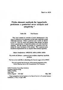
Let Ω0 be a domain in R3 that contains Ω∪U(Γ) and let K0,h be a quasiuniform partition of Ω0 into shape regular tetrahedra with mesh parameter h. See Fig. 1 for an illustration of the different domains. We consider a continuous piecewise linear approximation Γh of Γ such that Γh ∩ K is a subset of a hyperplane in R3 for each K ∈ K0,h . We assume that Γh ⊂ U(Γ) and that the following approximation assumptions hold: kρkL∞ (Γh ) . h2

(3.2)

kne − nh kL∞ (Γh ) . h

(3.3)

and where nh denotes the piecewise constant exterior unit normal to Γh . Finally, we define Ωh as the domain enclosed by Γh . These assumptions are consistent with the piecewise linear nature of the discrete surface. 4

U(Γ)

Ω

Γ Ω0

Figure 1: Illustration of the domain Ω, Ω0 , U(Γ), and Γ. The domain U(Γ) is the yellow region where for each x ∈ U(Γ) there is a unique closest point on Γ.

3.2

Finite Element Spaces

We define the following sets of elements KB,h = {K ∈ Kh,0 : K ∩ Ωh 6= ∅},

KS,h = {K ∈ Kh,0 : K ∩ Γh 6= ∅}

(3.4)

and the corresponding sets NB,h =

[

NS,h =

K,

K∈KB,h

[

K

(3.5)

K∈KS,h

We let V0,h be the space of piecewise linear continuous functions defined on K0,h . Next let VB,h = V0,h |NB,h ,

VS,h = V0,h |NS,h /h1Γh i,

Wh = VB,h × VS,h

(3.6)

be the spaces of continuous piecewise linear polynomials defined on NB,h and NS,h , respecR tively, where we also enforced Γh vS = 0 for v ∈ VS,h .

3.3

The Finite Element Method

The finite element method takes the form: find uh = (uB,h , uS,h ) ∈ Wh such that Ah (uh , v) = lh (v) ∀v ∈ Wh 5

(3.7)

Here the bilinear form is defined by Ah (v, w) = ah (v, w) + jh (v, w)

(3.8)

ah (v, w) = aB,h (vB , wB ) + aS,h (vS , wS ) + aBS,h (v, w)

(3.9)

with and

  aB,h (uB , vB ) = bB (kB ∇uB , ∇vB )Ωh aS,h (uS , vS ) = bS (kS ∇S uS , ∇S vS )Γh   aBS,h (u, v) = (bB uB − bS uS , bB vB − bS vS )Γh = (b · u, b · v)Γh

(3.10)

where ∇Γh = Ph ∇ and Ph = I − nh ⊗ nh . Next jh (v, w) is a stabilizing term of the form jh (v, w) = τB h3 jB (vB , wB ) + τS jS (vS , wS )

(3.11)

where τB , τS are positive parameters and, letting [x]|F denote the jump of x over the face F, X jB (vB , wB ) = ([nF · ∇vB ], [nF · ∇wB ])F (3.12) F ∈FB,h

jS (vS , wS ) =

X

F ∈FS,h

([nF · ∇vS ], [nF · ∇wS ])F

(3.13)

with FS,h the set of internal faces (i.e. faces with two neighbors) in KS,h and FB,h denotes the set of faces that are internal in KB,h and belong to an element in KS,h . Finally, the right hand side is defined by lh (v) = lB,h (vB ) + lS,h (vS ) = bB (fB,h , vB )Ωh + bS (fS,h , vS )Γh

(3.14)

with fB,h and fS,h discrete approximations of fB and fS that will be specified more precisely below. The purpose of the stabilization terms is to ensure that the resulting algebraic system of equations is well conditioned.

4

A Priori Error Estimates

Outline of the proof. To prove a priori error estimates we first construct a bijective mapping Fh that maps the exact domain to the approximate domain. The mapping is used to lift the discrete solution onto the exact domain where the error is evaluated. The construction of the mapping is based on a representation of the discrete boundary Γh as a normal function over the exact boundary Γ together with an extension to a small tubular δ neighborhood of the boundary. In the remainder of the domain Fh is the identity mapping. Next a Strang type lemma relates the error in the computed solution to an interpolation 6

error and quadrature errors emanating from the approximation of the domain. Using the assumptions on the approximation properties of the discrete surface we derive bounds on the quadrature errors. The surface quadrature errors are O(h2 ) while the bulk quadrature error is O(h) in the δ neighborhood and zero elsewhere. To establish an optimal order energy norm error estimate only first order estimates of the quadrature errors are needed but for L2 error estimates second order estimates are necessary. To achieve a second order estimate of the quadrature error we utilize the fact that δ can be chosen in the form δ = Ch with a sufficiently large C.

4.1

Mapping the Exact Domain to the Approximate Domain

The Mapping Fh : For δ > 0 let Uδ (Γ) be the open tubular δ neighborhood Uδ (Γ) = {x ∈ R3 : |ρ(x)| < δ}

(4.1)

For 0 < δ ≤ δ0 , where δ0 is a constant, that only depend on the domain, chosen such that Uδ0 (Γ) ⊂ U(Γ), the mapping Uδ (Γ) 3 x 7→ (p(x), ρ(x)) ∈ Γ × (−δ, δ)

(4.2)

Γ × (−δ, δ) 3 (x, z) 7→ x + zn(x) ∈ Uδ (Γ)

(4.3)

is a bijection with inverse

We next note that there is a function γh : Γ → R such that qh : Γ 3 x 7→ x + n(x)γh (x) ∈ Γh

(4.4)

is a bijection. Since for x ∈ Γh there holds p(x) = x − ne (x)ρ(x) we may deduce that qh (x) is the inverse mapping to p(x) : Γh 7→ Γ. Using the assumptions on the approximation properties (3.2) and (3.3) we obtain the following estimates (see Appendix) kγh kL∞ (Γ) . h2 ,

k∇Γ γh kL∞ (Γ) . h

(4.5)

Assuming that h is sufficiently small so that Γh ⊂ Uδ/3 (Γ) we may define the mapping Fh : Ω0 3 x 7→ x + χ(ρ(x))ne (x)γhe (x) ∈ Ω0

(4.6)

where χ : (−δ, δ) → [0, 1] is a smooth cut off function that equals 1 on (−δ/3, δ/3) and 0 on (−δ, δ) \ (−2δ/3, 2δ/3) and the derivative Dχ satisfies the estimate kDχkL∞ (−δ,δ) . δ −1

(4.7)

We note that by construction Fh : Ω0 → Ω0 is a bijection such that Fh (Ω) = Ωh ,

Fh (Γ) = Γh

(4.8)

and Fh = I

in Ω0 \ Uδ (Γ) 7

(4.9)

The Derivative DFh : The derivative DFh (x) ∈ L(R3 , R3 ) of Fh at x ∈ Ω0 is given by   e DFh (x) = I + χ(ρ(x))n (x) D(γhe (x)) (4.10)   + D(χ(ρ(x))ne (x)) γhe (x)   = I + χ(ρ(x))ne (x) (Dγh )e (x)Dp(x) (4.11)   + (Dχ)(ρ(x))Dρ(x)ne (x) γhe (x)   + χ(ρ(x))(Dn)e (x)Dp(x) γhe (x) Next we note that

Dρ = ne ,

Dn = HΓ ,

Dp = PΓe − ρHΓ

(4.12)

where we used the identity p(x) = x − ρ(x)Dρ(x) = x − ρ(x)ne (x) and introduced the curvature tensor HΓ (x) = ∇ ⊗ ∇ρ(x), x ∈ Γ. Note that it holds kHΓ kL∞ (Uδ (Γ) ) . 1 for δ small enough. Thus we have DFh (x) = I + χ(ρ(x))ne (x) ⊗ (∇Γ γh )e (x)(PΓe (x) − ρ(x)HΓ (x)) + γhe (x)(Dχ)(ρ(x))ne (x) ⊗ ne (x) + χ(ρ(x))γhe (x)HΓe (x)(PΓe (x) − ρ(x)HΓ (x))

(4.13)

On the surface Γ we have the simplified expression DFh (x) = I + n(x) ⊗ ∇Γ γh (x) + γh (x)HΓ (x)

(4.14)

since χ = 1 and Dχ = 0 in a neighborhood of Γ and ρ(x) = 0 for x ∈ Γ. We note that DFh (x) maps the tangent space Tx (Γ) into the piecewise defined tangent space TFh (x) (Γh ). In other words we have the identity DFh PΓ = (PΓh ◦ Fh )DFh PΓ

(4.15)

DFh,Γ (x) : Tx (Γ) 3 y 7→ (PΓh ◦ Fh )DFh PΓ y ∈ TFh (x) (Γh )

(4.16)

and the mapping

is invertible. Observing that by (4.5), DFh = I + O(h), for small enough h we have the bounds (4.17) kDFh kL∞ (Ω0 ,L(R3 ,R3 )) . 1, kDFh−1 kL∞ (Ω0 ,L(R3 ,R3 )) . 1 and

kDFh,Γ kL∞ (Γ,L(Tx (Γ),TFh (x) (Γh )) . 1,

−1 kDFh,Γ kL∞ (Γ,L(TFh (x) (Γh ),Tx (Γ)) . 1

(4.18)

Below we simplify the notation as follows kDFh kL∞ (Ω0 ) = kDFh kL∞ (Ω0 ,L(R3 ,R3 )) for the mappings DFh and DFh,Γ and their inverses. 8

The Jacobian Determinants J Fh and J Fh,Γ : We have the following relations between the measures on the exact and approximate surface and domain dΩh = JFh dΩ,

dΓh = JFh,Γ dΓ

(4.19)

where the Jacobian determinants are defined by JFh (x) = |det(DFh (x))| JFh,Γ (x) = |DFh,Γ (x)ξ1 × DFh,Γ (x)ξ2 |

(4.20) (4.21)

and {ξ1 , ξ2 } is an orthonormal basis in Tx (Γ). We note that JFh = 1 on Ω0 \ Uδ (Γ) and recall that DFh = I + O(h). Thus we have the following estimates in the bulk kJFh kL∞ (Ω0 ) . 1,

kJFh−1 kL∞ (Ω0 ) . 1,

k1 − JFh kL∞ (Uδ (Γ)) . h

(4.22)

since the determinant is a third order polynomial of the elements in DFh . On the surface we note that DFh,Γ (x)ξ = ξ + n(ξ · ∇Γ γh ) + γh HΓ · ξ ∀ξ ∈ Tx (Γ) (4.23)

where the last term is O(h2 ). The Jacobian determinant JFh,Γ is the norm of the cross product |DFh,Γ (x)ξ1 × DFh,Γ (x)ξ2 | = |(ξ1 + n(ξ1 · ∇Γ γh )) × (ξ2 + n(ξ2 · ∇Γ γh ))| + O(h2 ) = |n − ξ1 (ξ1 · ∇Γ γh ) − ξ2 (ξ2 · ∇Γ γh )| + O(h2 )  1/2 = 1 + (ξ1 · ∇Γ γh )2 + (ξ2 · ∇Γ γh )2 + O(h2 ) = 1 + O(h2 )

(4.24)

where we used the identities ξ1 × ξ2 = n, n × ξ2 = −ξ1 , ξ1 × n = −ξ2 , n × n = 0, the fact that {ξ1 , ξ2 , n} is a positively oriented orthonormal basis in R3 to compute the norm, and finally the estimate (1 + δ)1/2 ≤ 1 + δ/2, δ > 0 in the last step. We thus have the following estimates for the surface Jacobian kJFh,Γ kL∞ (Γ) . 1,

4.2

−1 kJFh,Γ kL∞ (Γ) . 1,

k1 − JFh,Γ kL∞ (Γ) . h2

(4.25)

Lifting to the Exact Domain

We define the lifting or pullback of v L with respect to Fh of a function v defined on Ω0 as follows v L := v ◦ Fh (4.26) We note in particular that any function defined on Ωh and Γh may be lifted to a function on Ω and Γ. Using the chain rule Dv L = D(v ◦ Fh ) = (Dv ◦ Fh )DFh = (Dv)L DFh 9

(4.27)

and thus we obtain the identities ∇v L = DFhT (∇v ◦ Fh ) = DFhT (∇v)L

(4.28)

∇Γ v L = PΓ ∇v L = PΓ DFhT (∇v)L

T = PΓ DFhT PΓLh (∇v)L = (PΓ DFhT PΓLh )(∇Γh v)L = DFh,Γ (∇Γh v)L

(4.29)

where DFh,Γ was defined in (4.16). Summarizing, we have the relations (∇v)L = DFh−T ∇v L

∇v L = DFhT (∇v)L ,

(4.30)

and −T (∇Γh v)L = DFh,Γ ∇Γ v L

T ∇Γ v L = DFh,Γ (∇Γh v)L ,

(4.31)

Using the bounds (4.17) and (4.18) we conclude that the following equivalences hold k∇v L kL2 (Ω) . k(∇v)L kL2 (Ω) . k∇v L kL2 (Ω)

(4.32)

k∇Γ v L kL2 (Γ) . k(∇Γh v)L kL2 (Γ) . k∇Γ v L kL2 (Γ)

(4.33)

and

4.3

Interpolation

Let EB : H 2 (Ω) → H 2 (Ω0 ) be an extension operator such that kEB vkH 2 (Ω0 ) . kvkH 2 (Ω)

(4.34)

and ES : H 2 (Γ) → H 2 (U(Γ)) be the extension operator such that ES v = v ◦ p. Then we have the estimate kES vkH 2 (Uδ (Γ)) . δ 1/2 kvkH 2 (Γ) (4.35) for any δ > 0 such that Uδ (Γ) ⊂ U(Γ). We finally define the extension operator E : H 2 (Ω) × H 2 (Γ) 3 (uB , uS ) 7→ (EB uB , ES uS ) ∈ H 2 (Ω0 ) × H 2 (U(Γ))

(4.36)

When suitable we simplify the notation and write u = Eu. We let πSZ,h : L2 (Ω0 ) → V0,h denote the standard Scott-Zhang interpolation operator and recall the interpolation error estimate kv − πSZ,h vkH m (K) ≤ Ch2−m kvkH 2 (N (K)) ,

m = 1, 2,

K ∈ K0,h

(4.37)

where N (K) ⊂ Ωh is the union of the neighboring elements of K. We then define the interpolant πh u = (πB,h uB , πS,h uS ) (4.38) where πB,h uB = (πSZ,h EB uB )|NB,h ∈ VB,h 10

(4.39)

and We use the notation

πS,h uS = (πSZ,h ES uS )|NS,h ∈ VS,h

(4.40)

πhL u = (πh u)L = (πh u) ◦ Fh

(4.41)

for the pullback of πh u to Ω by Fh . With these definitions we have the following lemma: Lemma 4.1 The following estimate holds |||u − πhL u||| . hkukH 2 (Ω)×H 2 (Γ)

(4.42)

Proof. Using a trace inequality we obtain L L |||u − πhL u|||2 = bB kB k∇(uB − πB,h uB )k2L2 (Ω) + bS kS k∇(uS − πS,h uS )k2L2 (Γ) L L + kbB (uB − πB,h uB ) − bS (uS − πS,h uS )k2L2 (Γ)

L L . kuB − πB,h uB k2H 1 (Ω) + kuS − πS,h uS k2H 1 (Γ)

= I + II

(4.43)

Term I. The first term may be estimated as follows L I = kuB − πB,h uB kH 1 (Ω) = kuB − (πSZ,h EB uB |Ωh )L kH 1 (Ω)

≤ kuB − (EB uB |Ωh )L kH 1 (Ω) + k((I − πSZ,h )EB uB |Ωh )L kH 1 (Ω) . hkuB kH 2 (Ω)

(4.44)

Here we used the Sobolev Taylor’s formula, see [2], to estimate the first term: consider first a function v ∈ H 2 (Ω0 ); then we have kv − v ◦ Fh kL2 (Ω0 ) . kI − Fh kL∞ (Ω0 ) k∇vkL2 (Ω0 ) . h2 kvkH 1 (Ω0 )

(4.45)

and for the derivative k∇(v − v ◦ Fh )kL2 (Ω0 )

= k∇v − DFhT (∇v ◦ Fh )kL2 (Ω0 )

≤ k∇v − (∇v ◦ Fh )kL2 (Ω0 ) + k(DFhT − I)(∇v ◦ Fh )kL2 (Ω0 )

. kI − Fh kL∞ (Ω0 ) k∇vkH 1 (Ω0 ) + k(DFhT − I)kL∞ (Ω0 ) k∇vkL2 (Ω0 ) . h2 kvkH 2 (Ω0 ) + hk∇vkL2 (Ω0 ) . hkvkH 2 (Ω0 )

(4.46)

Now we may apply these inequalities with v = EB uB and finally use the stability (4.34) of the extension operator EB . The second term in (4.44) is estimated by mapping to the discrete domain using the interpolation estimate (4.37) and then using the stability estimate (4.34). 11

Term II. Changing domain of integration from Γ to Γh and then using an element–wise trace inequality we obtain T L ∇Γh (ueS − πS,h uS )|JFh,Γ |−1/2 k2L2 (Γh ) uS )k2L2 (Γ) = kDFh,Γ k∇Γ (uS − πS,h X . h−1 kueS − πS,h uS kH 1 (K) + hkueS − πS,h uS k2H 2 (K) K∈KS,h

.

X

K∈KS,h

hkueS k2H 2 (N (K))

. h2 kuS k2H 2 (Γ)

(4.47)

Here we used the interpolation estimate (4.37) followed by the stability estimate (4.35) for the extension operator with δ ∼ h, which is possible since there is δ . h such that KS,h ⊂ Uδ (Γ). We also need the face norm |||v|||2F = h3 jB (vB,h , vB,h ) + jS (vS,h , vS,h ) X X k[nF · ∇vS k2L2 (F ) = h3 k[nF · ∇vB ]k2L2 (F ) + F ∈FB,h

(4.48) (4.49)

F ∈FS,h

for which we have the following interpolation error estimate. Lemma 4.2 The following estimate holds |||u − πh u|||F . hkukH 2 (Ω)×H 2 (Γ)

(4.50)

Proof. This estimate follows directly by using an element wise trace inequality, followed by the interpolation estimate (4.37), and finally the stability estimates (4.34) and (4.35) for the extension operators.

4.4

Strang’s Lemma

Lemma 4.3 The following estimate holds 

|||u − uLh |||2 + |||u − uh |||2F

1/2

 1/2 . |||u − πhL u|||2 + |||u − πh u|||2F + sup

v∈Wh

+ sup v∈Wh

12

a(uLh , v L ) − ah (uh , v) |||v L ||| l(v L ) − lh (v) |||v L |||

(4.51)

Proof. Adding and subtracting an interpolant πhL u, defined by (4.41), and using the triangle inequality we obtain  1/2  1/2 |||u − uLh |||2 + |||u − uh |||2F ≤ |||u − πhL u|||2h + |||u − πh u|||2F (4.52)  1/2 + |||πhL u − uLh |||h + |||πh u − uh |||2F

To estimate the second term we start from the coercivity  1/2 a(πhL u − uLh , v L ) + jh (πh u − uh , v) |||πhL u − uLh |||2 + |||πh u − uh |||2F ≤ sup (4.53)  1/2 v∈Wh \{0} 2 L 2 |||v ||| + |||v|||F Adding and subtracting the exact solution, and using Galerkin orthogonality the numerator may be written in the following form a(πhL u − uLh , v L ) + jh (πh u − uh , v)

= a(πhL u − u, v L ) + a(u − uLh , v L ) + jh (πh u − uh , v)

= a(πhL u − u, v L ) + l(v L ) − a(uLh , v L ) + jh (πh u − uh , v) = a(πhL u − u, v L ) + l(v L ) − lh (v)

+ ah (uh , v) + jh (uh , v) − a(uLh , v L ) + jh (πh u − uh , v)

= a(πhL u − u, v L ) + jh (πh u − u, v)     + ah (uh , v) − a(uLh , v L ) + l(v L ) − lh (v)

(4.54)

Using (4.53) and estimating the first term using the Cauchy-Schwarz inequality the lemma follows directly.

4.5

Estimate of the Quadrature Errors

Lemma 4.4 If h . δ ≤ δ0 and h is small enough. Then it holds |a(v L , wL ) − ah (v, w)| . h2 k∇Γ vSL kL2 (Γ) k∇Γ wSL kL2 (Γ) 2

L

(4.55)

L

+ h kb · v kL2 (Γ) kb · w kL2 (Γ)

L + hk∇vBL kL2 (Uδ (Γ)∩Ω) k∇wB kL2 (Uδ (Γ)∩Ω)

∀v, w ∈ Wh

Proof. Using the definition of the bilinear forms we have L a(v L , wL ) − ah (v, w) = aB (vBL , wB ) − aB,h (vB , wB ) | {z }

+

I L L aS (vS , wS ) −

|

= I + II + III

a (v , w ) + a (v, w) − aBS,h (v, w) {z S,h S S} | BS {z } II

13

III

(4.56)

We now proceed with estimates of the three terms. Term I. Starting from the definition of the forms (2.15) and (3.10), changing domain of integration to Ω, and using (4.30), we obtain the following identity L (bB kB )−1 (aB (vBL , wB ) − aB,h (vB , wB ))

= (DFhT (∇vB )L , DFhT (∇wB )L )Ω − (∇vB , ∇wB )Ωh

= (DFhT (∇vB )L , DFhT (∇wB )L )Ω − ((∇vB )L , (∇wB )L JFh )Ω = ((DFh DFhT − JFh I)(∇vB )L , (∇wB )L )Ω = (Ah,Ω (∇vB )L , (∇wB )L )Ω

(4.57)

In order to estimate Ah,Ω = DFh DFhT − JFh I we note that Ah,Ω = 0 in Ω0 \ Uδ (Γ) and in Uδ (Γ) we have the identity Ah,Ω = DFh DFhT − JFh I

= (DFh − I)(DFh − I)T + (DFh + DFhT ) − I − JFh I

= (DFh − I)(DFh − I)T + (DFh − I) + (DFh − I)T + (1 − JFh )I

(4.58)

and therefore we have the estimate kAh,Ω kL∞ (Uδ (Γ)∩Ω) . kDFh − Ik2L∞ (Uδ (Γ)∩Ω)

(4.59)

+ kDFh − IkL∞ (Uδ (Γ)∩Ω) + k1 − JFh kL∞ (Uδ (Γ)∩Ω)

This estimate holds for any 0 < δ ≤ δ0 and h such that Γh ⊂ Uδ/3 (Γ)

(4.60)

Recall that (4.60) is required in the definition (4.6) of the mapping Fh . Now using the assumption that there is a constant C1 > 0 such that C1 h < δ ≤ δ0 , there is a constant h0 > 0, independent of δ, such that (4.60) holds for 0 < h ≤ h0 , since we have the estimate kγh kL∞ (Γ) ≤ C2 h2 ≤ (C2 h0 )h < C1 h/3 < δ/3, where we may choose h0 such that C2 h0 < C1 /3. Proceeding with the estimate of kDFh − IkL∞ (Uδ (Γ)∩Ω) for C1 h < δ ≤ δ0 and 0 < h ≤ h0 we start from the identity (4.13) and then using the estimates kχkL∞ (−δ,δ) = 1, 0 < δ ≤ δ0 and kPΓe − ρHΓ kL∞ (Uδ0 (Γ)) . 1 we obtain kDFh − IkL∞ (Uδ (Γ)∩Ω) . k∇Γ γh kL∞ (Γ) + kγh kL∞ (Γ) kDχkL∞ (−δ,δ) + kγh kL∞ (Γ) . h + h2 δ −1 + h2 .h

14

(4.61)

where we used (4.5) and (4.7) and C1 h < δ. This estimate holds for all δ and h such that C1 h < δ ≤ δ0 and 0 < h ≤ h0 . Combining (4.61) with the estimate for the Jacobian determinant (4.22) we obtain the estimate kAh,Ω kL∞ (Uδ (Γ)∩Ω) . h

(4.62)

Ah,Ω = 0 in Ω \ Uδ (Γ)

(4.63)

and we also recall that Using the bound (4.62) for Ah,Ω we obtain the estimate |aB (v L , wL ) − aB,h (v, w)| . hk(∇v)L kL2 (Uδ (Γ)) k(∇w)L kL2 (Uδ (Γ)) . hk∇v L kL2 (Uδ (Γ)) k∇wL kL2 (Uδ (Γ))

(4.64)

At last we used the estimate k(∇v)L kL2 (Uδ (Γ)) = kDFh−T (∇v L )kL2 (Uδ (Γ))

(4.65)

= kDFh−T kL∞ (Uδ (Γ)) k∇v L kL2 (Uδ (Γ)) . k∇v L kL2 (Uδ (Γ))

where we employed (4.17). Term II. Proceeding in the same way and using (4.31) we obtain   (bS kS )−1 aS (vSL , wSL ) − aS,h (vS , wS ) = (∇Γ vSL , ∇Γ wSL )Γ − (∇Γh vS , ∇Γh wS )Γh

T T = (DFh,Γ (∇Γh vS )L , DFh,Γ (∇Γh wS )L )Γ − ((∇Γh vS )L , (∇Γh wS )L JFh,Γ )Γ T = ((DFh,Γ DFh,Γ − PΓLh JFh,Γ )(∇Γh vS )L , (∇Γh wS )L )Γ

= (AΓ,h (∇Γh vS )L , (∇Γh wS )L )Γ

(4.66)

where we introduced T AΓ,h = DFh,Γ DFh,Γ − PΓLh JFh,Γ

(4.67)

Using the definition (4.16) of DFh,Γ and the expression (4.14) for DFh we have the identity DFh,Γ = PΓLh DFh PΓ = PΓLh (I + n ⊗ ∇Γ γh + γh HΓ )PΓ

= PΓLh PΓ + (PΓLh n) ⊗ ∇Γ γh + γh PΓLh HΓ PΓ

(4.68)

Here the second term can be estimated as follows k(PΓLh n) ⊗ ∇Γ γh kL∞ (Γ) . kPΓLh nkL∞ (Γ) k∇Γ γh kL∞ (Γ) . h2 15

(4.69)

where we used the estimate kPΓLh nkL∞ (Γ) = kPΓLh (n − nLh )kL∞ (Γ) . kn ◦ p − nh kL∞ (Γh ) . h

(4.70)

For the third term we have the estimate kγh PΓLh HΓ PΓ kL∞ (Γ) . kγh kL∞ (Γ) kPΓLh kL∞ (Γ) kHΓ kL∞ (Γ) kPΓ kL∞ (Γ) . h2

(4.71)

Thus we conclude that DFh,Γ = PΓLh PΓ + O(h2 )

(4.72)

Inserting this identity into the expression (4.67) for AΓ,h and using the identity PΓLh JFh,Γ = PΓLh + PΓLh (JFh,Γ − 1) = PΓLh + O(h2 )

(4.73)

where we used (4.25), we obtain AΓ,h = PΓLh PΓ PΓLh − PΓLh + O(h2 )

(4.74)

Now the following identity holds PΓLh PΓ PΓLh − PΓLh = PΓLh (PΓ − PΓLh )(PΓ − PΓLh )PΓLh

(4.75)

which leads to the estimate kPΓLh PΓ PΓLh − PΓLh kL∞ (Γ) ≤ kPΓLh k2L∞ (Γ) kPΓ − PΓLh k2L∞ (Γ) . h2

(4.76)

where we used the bound kPΓ − PΓLh kL∞ (Γ) = kn ⊗ n − nLh ⊗ nLh kL∞ (Γ)

. k(n − nLh ) ⊗ nkL∞ (Γ) + knLh ⊗ (n − nLh )kL∞ (Γ) . kne − nh kL∞ (Γh ) .h

Thus we finally arrive at kAΓ,h kL∞ (Γ) . h2

(4.77)

and therefore we have the estimate |aS (v L , wL ) − aS,h (v, w)| . h2 k(∇Γh v)L kL2 (Γ) k(∇Γh w)L kL2 (Γ) . h2 k∇Γ v L kL2 (Γ) k∇Γ wL kL2 (Γ)

where at last we used (4.18).

16

(4.78)

Term III. We have aBS (v L , wL ) − aBS,h (v, w) = (b · v L , b · wL )Γ − (b · v, b · w)Γh = ((1 − JFΓ,h )b · v L , b · wL )Γ

and thus we obtain the estimate

|aBS (v L , wL ) − aBS,h (v, w)| . h2 kb · v L kL2 (Γ) kb · wL kL2 (Γ)

(4.79) (4.80)

Lemma 4.5 If fh = (fB,h , fS,h ) satisfies the estimate L L kfB − fB,h kL2 (Ω) + kfS − fS,h kL2 (Γ) . h2

(4.81)

Then it holds |l(v L ) − lh (v)| . h2 kv L kL2 (Ω)×L2 (Γ)

∀v ∈ Wh

(4.82)

Proof. We have l(v L ) − lh (v) = bB (fB , vBL )Ω − bB (fB,h , vB )Ωh + bS (fS , vSL )Γ − bS (fS,h , vS )Γh L L = bB (fB − fB,h JFh , vBL )Ω + bS (fS − fS,h JFh , vSL )Γ

(4.83)

which immediately leads to the estimate

|l(v L ) − lh (v)| . h2 kv L kL2 (Ω)×L2 (Γ)

4.6

(4.84)

Error Estimates

Theorem 4.1 The following error estimate holds  1/2 L 2 2 |||u − uh ||| + |||u − uh |||F . hkukH 2 (Ω)×H 2 (Γ)

(4.85)

for small enough mesh parameter h.

Proof. Using the Strang Lemma, Lemma 4.3, in combination with the quadrature error estimates in Lemma 4.4 and 4.5, we obtain 1/2  1/2  |||u − uLh |||2 + |||u − uh |||2F . |||u − πhL u|||2 + |||u − πh u|||2F a(uLh , v L ) − ah (uh , v) l(v L ) − lh (v) + sup + sup |||v L ||| |||v L ||| v∈Wh v∈Wh  1/2 . |||u − πhL u|||2 + |||u − πh u|||2F + h|||uLh ||| + h2 .h

(4.86)

17

Here we used the interpolation error estimates in Lemma 4.1 and Lemma 4.2, and the stability estimate |||uLh ||| . kf kL2 (Ω)×L2 (Γ) (4.87) in the last inequality. Theorem 4.2 The following error estimate holds ku − uLh kL2 (Ω)×L2 (Γ) . h2 kukH 2 (Ω)×H 2 (Γ)

(4.88)

for small enough mesh parameter h. Proof. Let φ be the solution to the dual problem: find φ ∈ W such that a(v, φ) = (v, ψ)L2 (Ω)×L2 (Γ)

∀v ∈ W

(4.89)

where ψ = (ψB , ψS ) ∈ L2 (Ω) × L2 (Γ). Then we have the regularity estimate kφkH 2 (Ω)×H 2 (Γ) . kψkL2 (Ω)×L2 (Γ)

(4.90)

Setting v = u − uLh , and adding and subtracting suitable terms we obtain (uB − uLB,h , ψB )Ω + (uS − uLS,h , ψS )Γ = a(u − uLh , φ)

= a(u − uLh , φ − πhL φ) + a(u − uLh , πhL φ)   = a(u − uLh , φ − πhL φ) + l(πhL φ) − lh (πh φ) {z } | | {z } I II   + ah (uh , πh φ) − a(uLh , πhL φ) + jh (uh , πh φ) {z } {z } | IV | III

= I + II + III + IV

(4.91)

Term I. Using Cauchy-Schwarz, the energy norm estimate (4.85), the interpolation estimate (4.42) we obtain |I| ≤ |||u − uLh ||| |||φ − πhL φ||| . h2 kψkL2 (Ω)×L2 (Γ)

(4.92)

Term II. Using Lemma 4.5 we immediately get |II| . h2 kψkL2 (Ω)×L2 (Γ)

18

(4.93)

Term III. Using Lemma 4.4 we obtain L |a(uLh , πhL φ) − ah (uLh , πhL φ)| . h2 k∇Γ uLS,h kL2 (Γ) k∇Γ πS,h φS kL2 (Γ)

+ h2 kb · uLh kL2 (Γ) kb · πhL φkL2 (Γ)

L + hk∇uLB,h kL2 (Uδ (Γ)∩Ω) k∇πB,h φB kL2 (Uδ (Γ)∩Ω)

(4.94)

for h . δ ≤ δ0 and h small enough. To show that the third term is actually of second order we shall use the Poincar´e inequality kvkL2 (Uδ (Γ)∩Ω) . (δ/δ0 )1/2 kvkH 1 (Uδ0 (Γ)∩Ω) ,

0 < δ ≤ δ0

(4.95)

See [7] for a proof of this inequality. We proceed in the following way L L k∇πB,h φB kL2 (Uδ (Γ)∩Ω) ≤ k∇(πB,h φB − φB )kL2 (Uδ (Γ)∩Ω) + k∇φB kL2 (Uδ (Γ))

. (h + δ 1/2 )kφB kH 2 (Uδ0 (Γ)∩Ω) . (h + h1/2 )kφB kH 2 (Ω)

(4.96)

where we used the fact that δ can actually be chosen such that δ ∼ h, see Lemma 4.4, and the interpolation error estimate (4.42). The term k∇uLB,h kL2 (Uδ (Γ)) can be estimated using the same technique but we employ the energy norm error estimate (4.85) instead k∇uLB,h kL2 (Uδ (Γ)∩Ω) . k∇(uLB,h − uB )kL2 (Uδ (Γ)∩Ω) + k∇uB kL2 (Uδ (Γ)∩Ω) . |||u − uh ||| + δ 1/2 k∇uB kL2 (Uδ (Γ)∩Ω) . (h + h1/2 kukH 2 (Ω)×H 2 (Γ)

(4.97)

Combining (4.96) and (4.97) we obtain III . (h2 + h(h + h1/2 )2 )kψkL2 (Ω)×L2 (Γ) . h2 kψkL2 (Ω)×L2 (Γ)

(4.98)

Term IV . Using the fact that the jump term is consistent we obtain |IV | = |jh (u − uh , φ − πh φ)| ≤ |||u − uh |||F |||φ − πh φ|||F . h2 kψkL2 (Ω)×L2 (Γ)

(4.99)

where we used the energy estimate in Theorem 4.1 and the interpolation estimate in Lemma 4.1. We conclude the proof by collecting the estimates of Terms I − IV and taking the supremum over all ψ such that kψkL2 (Ω)×L2 (Γ) = 1.

5

Estimate of the Condition Number

Due to the different dimensions of the two coupled differential equations at the surface we shall see that it is natural to precondition the system in such a way that we seek (vB,h , vS,h ) such that the solution (uB,h , uS,h ) of (3.7) is given by (uB,h , uS,h ) = (vB,h , h1/2 vS,h ) 19

(5.1)

The corresponding variational problem for vh = (vB,h , vS,h ) takes the form: find v = (vB , vS ) ∈ Wh such that ˜ h (w) ∀w ∈ Wh A˜h (v, w) = L (5.2) where the bilinear forms are defined by A˜h (v, w) = Ah ((vB , h1/2 vS ), (wB , h1/2 wS )),

˜ h (w) = Lh ((wB , h1/2 wS )) L

(5.3)

We shall now estimate the condition number of the stiffness matrix A˜ associated with NS B the bilinear form A˜h (·, ·). Let {ϕB,i }N i=1 and {ϕS,i }i=1 be the standard piecewise linear basis functions in VB,h and VS,h ⊕ h1Γh i, respectively. Note that we have added the one dimensional space h1Γh i of constant functions on Γh . Define the following basis in the product space VB,h × VS,h ⊕ h1S,h i: ( (ϕB,i , 0) 1 ≤ i ≤ NB (5.4) ϕi = (0, ϕS,i−NB ) 1 + NB ≤ i ≤ N = NB + NS The expansion v =

PN

i=1

vbi ϕi defines an isomorphism

VB,h × VS,h /h1Γh i ⊕ h1S,h i → RNB × RNS /h1RNS i ⊕ h1RNS i vB , vbS ⊕ v S 1RNS ) (vB , vS ⊕ v S 1S,h ) 7→ (b

(5.5) (5.6)

kvk2h = kvB k2L2 (NB,h ) + kvS k2L2 (NS,h )

(5.7)

R where vS is the unique element in the equivalence classes of VS,h /h1Γh i with Γh vS = 0 and R v S = |Γh |−1 Γh vS is the meanvalue of vS . If we introduce the mesh dependent L2 -norm

where the sets NB,h and NS,h are defined in (3.5), we have the following standard estimate ch−d kvk2h . |b v |2N . Ch−d kvk2h

(5.8)

Let A˜ be the stiffness matrix with elements aij = A˜h (ϕi , ϕj ) + Jh (ϕi , ϕj ). The stiffness matrix is symmetric and has a one dimensional kernel consisting of a constant functions v = (vB , vS ), that satisfy b · v = bB vB − bS vS = 0. We shall estimate the condition number of A˜ as an operator on the invariant space V = RNB × RNS /h1RNS i defined by ˜ = |A| ˜ V |A˜−1 |V κ(A)

P 2 N ˜ V = supX∈V \{0} where |x|2N = N and |A| i=1 xi for x ∈ R introduce the discrete energy norm

(5.9) ˜ N |Ax| |x|N

for A˜ ∈ RN ×N . Next we

|||v|||2h = Ah (v, v) = ah (v, v) + jh (v, v)

(5.10)

The proof of the estimate of the condition number follow the approach presented in [8] and rely on a Poincar´e and an inverse inequality which we prove next. 20

Lemma 5.1 (Poincar´e inequality) Independently of the mesh/boundary intersection it holds that k(vB , vS )kh . |||(vB , h1/2 vS )|||h ∀(vB , vS ) ∈ Wh (5.11) Proof. Using Lemma 3.3 in [5] and then adding and subtracting suitable terms and using the triangle inequality followed by a Poincar´e inequality we obtain kvS k2L2 (NS,h ) . hkvS k2L2 (Γh ) + hjS (vS , vS )

. hk∇Γh vS k2L2 (Γh ) + jS (h1/2 vS , h1/2 vS )

. |||(vB , h1/2 vS )|||2h

(5.12)

R

Note that the Poincar´e inequality is applicable on Γh since Γh vS = 0. Next using the control provided by the jump term JB (·, ·) followed by a Poincar´e inequality we obtain kvB k2L2 (NB,h ) . kvB k2L2 (Ωh ) + h3 jB (vB , vB )

. kP0 vB k2L2 (Ωh ) + k∇vB k2L2 (Ωh ) + h3 JB (vB , vB ) . kP0 vB k2L2 (Γh ) + |||(vB , h1/2 vS )|||2h

. k(I − P0 )vB k2L2 (Γh ) + kvB k2L2 (Γh ) + |||(vB , h1/2 vS )|||2h 1/2 . k∇vB k2L2 (Ωh ) + b−2 vS k2L2 (Γh ) B kbB vB − bS h 2 1/2 + b−2 vS k2L2 (Γh ) + |||(vB , h1/2 vS )|||2h B bS kh

1/2 . b−2 vS k2L2 (Γh ) + |||(vB , h1/2 vS )|||2h B kh

(5.13)

Here P0 vB is the L2 -projection of vB onto constant functions on Ωh and we added and subtracted suitable functions to control P0 vB using the coupling term together with the control of kh1/2 vS k2Γh provided by (5.12) and the fact that the constant bB > 0. Furthermore, the first inequality in (5.13) is a consequence of the inverse inequality kvk2L2 (K1 ) . kvk2L2 (K2 ) + h3 k[nF · ∇v]k2L2 (F )

∀v ∈ VB,h

(5.14)

that holds for each pair of elements K1 and K2 that share a face F . Iterating the inequality (5.14) we may control the elements at the boundary in terms of the elements in the interior of Ωh as follows kvk2L2 (K1 )

.

kvk2L2 (KN )

+

N −1 X i=1

h3 k[nF · ∇v]k2L2 (Fi )

∀v ∈ VB,h

(5.15)

see [11] for further details. Note that for sufficiently small mesh size the length N of the shortest chain of elements that share an edge between an element that intersects the boundary and an interior element is uniformly bounded. Combining the two estimates (5.12) and (5.13) the lemma follows directly.

21

Lemma 5.2 (Inverse inequality) Independently of the mesh/boundary intersection it holds that |||(vB , h1/2 vS )|||2h . h−2 k(vB , vS )k2h ∀(vB , vS ) ∈ Wh (5.16) Proof. Using standard estimates we obtain the following three estimates bB kB k∇vB k2L2 (Ωh ) + τB h3 jB (vB , vB ) . h−2 kvB k2L2 (NB,h ) . h−2 k(vB , vS )k2h

(5.17)

kbB vB − bS h1/2 vS k2L2 (Γh ) . h−1 bB kvB k2L2 (NS,h ) + bS kvS k2L2 (NS,h ) . h−2 k(vB , vS )k2h

(5.18)

bS kS hk∇Γh vS k2L2 (Γh ) + τS hjS (vS , vS )) . (bS kS + τS )k∇vS k2L2 (NS,h ) . h−2 kvS k2L2 (NS,h )

and thus the proof is complete.

Finally, we are ready to prove our final estimate of the condition number. Theorem 5.1 The following estimate of the condition number of the stiffness matrix holds independently of the mesh/boundary intersection ˜ . h−2 κ(A) (5.19) ˜ V and |A˜−1 |V . Starting with |A| ˜ V we have Proof. We need to estimate |A| ˜v )N b Ab ˜v |V = sup (w, |Ab |w| bN w∈R b N = sup

w∈Wh

Ah ((vB , h1/2 vS ), (wB , h1/2 wS )) |||(wB , h1/2 wS )|||h k(wB , wS )kh |||(wB , h1/2 wS )|||h k(wB , wS )kh |w| bN

. h(d−2)/2 |||(vB , h1/2 vS )|||h . hd−2 |b v |N

(5.20)

where at last we used the estimate |||(vB , h1/2 vS )|||h . h−1 k(vB , vS )kh . h(d−2)/2 |b v |N

(5.21)

˜ V . hd−2 |A|

(5.22)

together with (5.16) and (5.8). Thus

Next we turn to the estimate of |A˜−1 |V . Using (5.8) and (5.11), we get

|b v |2N . h−d |||(vB , h1/2 vS )|||2h . h−d Ah ((vB , h1/2 vS ), (vB , h1/2 vS )) ˜v )N . h−d |b ˜v |N . h−d (b v , Ab v |N |Ab

˜v |N . Setting vb = A˜−1 w and thus we conclude that |b v |N ≤ Ch−d |Ab b we obtain −1 −d |A˜ |N . h

˜ N and |A˜−1 |N the theorem follows. Combining estimates (5.22) and (5.24) of |A| 22

(5.23)

(5.24)

1 1.5

0.5

z

1

0

0.5

−0.5

0

−1 −1

x

0 0 y

1 −1

1

Figure 2: The solution uS,h with h = 0.13125.

6

Numerical results

We consider an example where the domain Ω is the unit sphere, kB = kS = 1, bB = bS = 1, and fB and fS are choosen such that the exact solution is as in [7] given by uB = e(−x(x−1)−y(y−1)) uS = (1 + x(1 − 2x) + y(1 − 2y))e(−x(x−1)−y(y−1))

(6.1)

We study the convergence rate of the numerical solution uh = (uB,h , uS,h ) and the condition number of the system matrix using the proposed finite element method. A direct solver is used to solve the linear systems. The stabilization parameters τB = τS = 10−2 . We use a structured mesh for Ω0 and the mesh parameter h = hx = hy = hz . To represent the boundary Γ we use the standard level set method. We define a piecewise linear approximation to the distance function on K0,h and Γ is approximated as the zero level set of this approximate distance function. Thus, Γh is represented by linear segments on K0,h . The normal vectors are computed from the linear segments. The solution uS,h with h = 0.13125 and the triangulation of Γh are shown in Fig. 2. The convergence of uh in both the L2 norm and the H 1 norm are shown in Fig. 3. We have as expected first order convergence in the H 1 norm and second order convergence in the L2 norm. The spectral condition number of the matrix A˜ associated with the bilinear form A˜h (·, ·) (see equation (5.3)) is shown for different mesh sizes in Fig. 4.

23

−2

−4

−6

  log kueS − uS,hkL2(Γh)   log kueB − uB,hkL2(Ωh)
log h2

−8

−10 −4.5

1 0 −1

−4

−3.5

−3 log(h)

−2.5

−2

−2.5

−2

  log kueS − uS,hkH 1(Γh)   log kueB − uB,hkH 1(Ωh)

log(2h)

−2 −3 −4 −5 −4.5

−4

−3.5

−3 log(h)

Figure 3: Convergence of uB and uS . Upper panel: The error measured in the L2 norm versus mesh size. Lower panel: The error measured in the H 1 norm versus mesh size.

24

16

Condition number

14

12

10

8

−4

−3

−2

−1

log(h)

Figure 4: The spectral condition number of the matrix A˜ versus mesh size. The dashed line is proportional to h−2 .

Appendix Here we will give some details on the inequalities (4.5). First we recall that qh (x) = x + γh (x)n(x) x ∈ Γ

(6.2)

Now using the defintion of the closest point mapping y = p(y) + ρ(y)ne (y) y ∈ Γh

(6.3)

Setting x = p(y) in (6.2) we have y = p(y) + γh (p(y))ne (y) y ∈ Γh

(6.4)

and therefore, by uniqueness, ρ(y) = γh (p(y)), ∀y ∈ Γh . Thus we have γh = ρL and we immediately obtain the first inequality in (4.5) since kγh kL∞ (Γ) = kρL kL∞ (Γ) = kρkL∞ (Γh ) . h2

(6.5)

Next using (4.31) we have the identity T T (PΓh ne )L ∇Γ γh = ∇Γ ρL = DFh,Γ (∇Γh ρ)L = DFh,Γ

(6.6)

Estimating the right hand side using (4.18) and (4.70) we finally obtain k∇Γ γh kΓ . k∇Γh ρkΓh . kPΓh ne kΓh . h which is the second bound in (4.5). 25

(6.7)

References [1] M. R. Booty and M. Siegel, A hybrid numerical method for interfacial fluid flow with soluble surfactant, J. Comput. Phys. 229 (2010) 3864–3883. [2] S. C. Brenner and L. R. Scott, The mathematical theory of finite element methods, Springer Verlag, 3rd ed. (2008). [3] E. Burman; S. Claus, P. Hansbo, M. G. Larson, A. Massing, CutFEM: discretizing geometry and partial differential equations, Int. J. Num. Meth. Engrg. Submitted. 2014. [4] E. Burman; P. Hansbo, Fictitious domain finite element methods using cut elements: II. A stabilized Nitsche method, Appl. Numer. Math. 62 (4) (2012) 328–341. [5] E. Burman, P. Hansbo, M. G. Larson, A stable cut finite element method for partial differential equations on surfaces: the Laplace-Beltrami operator, arXiv:1312.1097 (2013). [6] G. Dziuk and C. M. Elliott, Finite element methods for surface PDEs, Acta Numerica, 22, (2013), pp 289 –396 [7] C. M. Elliott and T. Ranner, Finite element analysis for a coupled bulk-surface partial differential equation, IMA J. Numer. Anal. 33 (2) (2013) 377–402. [8] A. Ern, J. L. Guermond, Evaluation of the condition number in linear systems arising in finite element approximations, ESAIM: Mathematical Modelling and Numerical Analysis 40 (01), 29–48. [9] Y. Georgievskii, E. S. Medvedev, and A. A. Stuchebrukhov, Proton transport via the membrane surface, Biophys J. 82(6) (2002) 2833-2846. [10] P. Hansbo, M. G. Larson, and S. Zahedi, A cut finite element method for a Stokes interface problem, arXiv:1205.5684, (2012). [11] A. Massing, M. G. Larson, A. Logg and M. E. Rognes, A stabilized Nitsche fictitious domain method for the Stokes problem, arXiv:1206.1933, accepted for publication in Journal of Scientic Computing, (2013). [12] M. A. Olshanskii, A. Reusken, J. Grande, A finite element method for elliptic equations on surfaces, SIAM J. Numer. Anal. 47 (2009) 3339 – 3358. [13] M. A. Olshanskii, A. Reusken, A finite element method for surface PDEs: matrix properties, Numer. Math. 114 (3) (2010) 491–520 .

26