Paul Houston. This paper presents an ... aPaper presented as Invited Lecture at the State of the Art in Numerical Analysis. Conference, in York ... Subsequent sections of the paper are devoted to discussing an alternative, more direct, approach ...
Report no. 96/09
Finite element methods for hyperbolic problems: a posteriori error analysis and adaptivity a Endre Suli
Paul Houston
This paper presents an overview of recent developments in the area of a posteriori error estimation for rst-order hyperbolic partial di�erential equations. Global a posteriori error bounds are derived in the H 1 norm for steady and unsteady nite element and nite volume approximations of hyperbolic systems and scalar hyperbolic equations. We also consider the problem of a posteriori error estimation for linear functionals of the solution. The a posteriori error bounds are implemented into an adaptive nite element algorithm. Subject classi cations: AMS(MOS): 65M15, 65M50, 65M60 Key words and phrases: a posteriori error analysis, adaptivity, hyperbolic problems The rst author would like to acknowledge the nancial support of the EPSRC. The work reported here forms part of the research programme of the Oxford{Reading Institute for Computational Fluid Dynamics. Oxford University Computing Laboratory Numerical Analysis Group Wolfson Building Parks Road Oxford, England OX1 3QD May, 1996 a Paper presented as Invited Lecture at the State of the Art in Numerical Analysis Conference, in York, 1-4 April 1996.
2
Contents
1 Introduction 2 Johnson's paradigm 3 A posteriori error analysis for steady hyperbolic PDEs
3 4 7
3.1 Symmetric hyperbolic systems : : : : : : : : : : : : : : : : : : : : 7 3.2 A posteriori bound on the global error : : : : : : : : : : : : : : : 11 3.3 Application to the cell vertex nite volume method : : : : : : : : 12
4 A posteriori error estimation for linear functionals 5 Unsteady problems
5.1 A posteriori error analysis : : : : : : : : : : : : : : : : : : : : : 5.1.1 Error representation : : : : : : : : : : : : : : : : : : : : 5.1.2 Interpolation/projection estimates for the dual problem : 5.1.3 Strong stability of the dual problem : : : : : : : : : : : : 5.1.4 Completion of the proof of the a posteriori error estimate 5.2 Computational implementation : : : : : : : : : : : : : : : : : : 5.2.1 Adaptive algorithm : : : : : : : : : : : : : : : : : : : : : 5.2.2 Mesh modi cation strategy : : : : : : : : : : : : : : : : 5.3 Numerical experiments : : : : : : : : : : : : : : : : : : : : : : :
6 Conclusions References
: : : : : : : : :
14 19
21 21 22 23 24 25 26 28 28
29 31
3
1 Introduction Partial di�erential equations of hyperbolic type are of fundamental importance in many areas of applied mathematics, particularly uid dynamics and electromagnetics. Solutions to these equations exhibit localised phenomena, such as propagating discontinuities and sharp transition layers, and their reliable numerical approximation presents a challenging computational task; indeed, in order to resolve such localised features in an accurate and e�cient manner it is essential to use adaptively re ned computational meshes whose construction is governed by sharp a posteriori error bounds. Over the last decade the a posteriori error analysis of nite element methods for partial di�erential equations of hyperbolic and nearly-hyperbolic character has been a subject of intensive research. For an overview of current activity in this area we refer to the article of Johnson [11]; see also, [10], [12], [13], and references therein. The approach proposed in those papers, and reviewed in the next section, rests on performing an elliptic regularisation of the hyperbolic problem and exploiting the smoothing properties of the resulting adjoint problem in conjunction with Galerkin orthogonality. Subsequent sections of the paper are devoted to discussing an alternative, more direct, approach to the a posteriori error analysis of nite element approximations of hyperbolic problems which avoids the need for regularisation. Because of the inherent lack of strong smoothing properties in hyperbolic problems, particular care has then to be taken about existence of traces and integrationby-parts formulae which the a posteriori error analysis relies on; the necessary functional-analytic prerequisites that concern these issues are reviewed in the third section. By exploiting this theory, we derive a posteriori bounds on the global error in the H 1 norm for a general class of nite element methods (including certain nite volume schemes, interpreted as Petrov-Galerkin methods) for symmetric hyperbolic systems. For related work, see [15], [16], [17], [21], [25]. Controlling the computational error in a given norm, however, is not always the ultimate goal in practice. Indeed, in many engineering problems the accurate approximation of particular linear functionals of the solution (such as the lift, the drag, and the ux across the boundary of the domain) is at least as important as the reliable approximation of the solution in a given norm over the entire computational domain. We show, by considering the example of estimating the normal
ux through the boundary, how problems of this kind may be approximated in an e�cient way by exploiting a hyperbolic duality argument in conjunction with theoretical results concerning the propagation of singularities. In the nal part of the paper we discuss unsteady hyperbolic problems. In particular, we consider the a posteriori error analysis of a class of evolutionGalerkin methods for multi-dimensional scalar hyperbolic equations on a spatial domain and nite time interval [0; T ]. Here, we derive an a posteriori bound on the global error in the norm of the space L1(0; T ; H 1( )). We conclude by indicating the practical relevance of this work and by illustrating the implementation
4 of the a posteriori analysis into an adaptive evolution-Galerkin algorithm.
2 Johnson's paradigm In this brief section we review, in the context of rst-order hyperbolic systems, the general theoretical framework of a posteriori error estimation pursued by Johnson and his co-workers; for a comprehensive account, see [11] and [13]. Suppose that M is a Hilbert space with inner product (�; �) and let A : M ! M be a linear operator on M with domain D(A) � M and range R(A) = M (in our case a system of rst-order hyperbolic di�erential operators). Given that f 2 M, consider the problem of nding u 2 D(A) such that Au = f: In order to construct a Galerkin approximation to this problem, we consider a sequence of nite-dimensional spaces fU hg, parameterised by the positive discretisation parameter h; for the sake of simplicity we shall suppose that U h � D(A) for each h. Simultaneously, consider a sequence of nite-dimensional spaces fMhg, with Mh contained in M for each h. For the purposes of this paper, U h and Mh can be thought of as standard nite element spaces consisting of piecewise polynomial functions on a partition, of granularity h, of the computational domain. Let �h denote the orthogonal projector in M onto Mh. The Galerkin approximation uh of u is then sought in U h as the solution of the nite-dimensional problem �hAuh = �hf: In order to obtain a computable bound on the global error eh = u uh in terms of the residual rh, de ned by rh = f Auh; we begin by observing the Galerkin orthogonality property (rh; vh) = 0 8vh 2 Mh: This will be a key ingredient in the analysis. In addition, denoting by A� the adjoint of A, we consider the following auxiliary problem, referred to as the dual problem: A�� = u uh: The a posteriori error analysis is based on a duality argument, and it proceeds as follows: ku uhk2 = (u uh; u uh) = (u uh; A��) = (A(u uh); �) = (Au Auh; �) = (f Auh; �) = (rh; �):
5 By virtue of the Galerkin orthogonality property (rh; �h) = 0 for any �h 2 Mh, and therefore ku uhk2 = (rh; � �h) = (hsrh; h s(� �h)); where s is a non-negative real number, to be chosen below. By virtue of the Cauchy-Schwarz inequality, ku uhk2 � khsrhk kh s(� �h))k: While the rst term on the right-hand side is of the desired form, involving the (computable) residual rh multiplied by an appropriate power of the discretisation parameter, the second term incorporates �, the solution to the dual problem. Since the dual-problem has the global error as data, � is unknown and has to be eliminated from the analysis by relating it to u uh; furthermore a suitable choice of �h has to be made. This is achieved as follows: suppose that fW� g��0 is a scale of Hilbert spaces, with associated norms jjj � jjj� , such that W0 = M and W�2 is continuously embedded into W�1 whenever �2 � �1 . Furthermore, we assume that there exist �h 2 Mh and a positive constant Cz such that, for � 2 Ws , kh s(� �h)k � Czjjj�jjjs: For nite element methods, this hypothesis is easily ful lled by choosing Ws as a hilbertian Sobolev space of index s and referring to standard approximation properties of piecewise polynomial functions in Sobolev spaces, with �h taken as the projection, the interpolant or the quasi-interpolant of � from Mh. Thereby we arrive at the bound
ku uhk2 � Czkhsrhk jjj�jjjs: This brings us to the nal, and most important, step in the a posteriori error analysis. The norm jjj�jjjs appearing on the right-hand side of the last inequality has to be eliminated in terms of u uh by recalling the relationship between � and u uh, namely that A�� = u uh. Thus to proceed, we assume that A� is invertible and that (A�) 1 is a bounded linear operator from M to Ws ; hence jjj�jjjs = jjj(A�) 1(u uh)jjjs � C?ku uhk; where C? is a positive constant, greater than or equal to the norm of (A� ) 1. Finally, combining the last two bounds we arrive at the desired a posteriori bound on the global error eh = u uh in terms of the computable residual rh:
ku uhk � CzC?khsrhk:
In order to turn this into an error bound that can be used in practice, the constants Cz and C? have to be determined. Estimating Cz is a relatively simple matter using readily available results from approximation theory (see, for
6 example, Exercise 3.1.2 in Ciarlet's monograph [5] for an explicit formula for Cz in the case of standard nite element spaces consisting of continuous piecewise polynomials on simplices, or the work of Handscomb [7] for very much sharper estimates of Cz for piecewise linear nite elements on triangles). On the other hand, supplying C? is much harder, involving an analytical study of the wellposedness of the dual problem. Since any value of C? that is arrived at through such general analytical arguments is necessarily a considerable overestimate of the ratio jjj�jjjs=ku uhk, in practice the stability constant C? is determined computationally for the problem at hand, as part of the process of a posteriori error estimation. Finally, we have to x s, the exponent of h in the error bound. As one would like the a posteriori bound to re ect the approximation property of the space Mh to its full extent, one would wish to choose s as large as possible; unfortunately, for linear rst-order hyperbolic systems consisting of m equations on a domain � Rd , (A� ) 1 is a bounded operator from M = [L2 ( )]m to M = W0 = [L2 ( )]m only, so s cannot exceed 0; thus we end up with the bound
ku uhk � CzC? krhk: In fact, we note that when s = 0 there is no bene t in exploiting Galerkin orthogonality, and we may simply take �h = 0 in our argument to improve this bound to ku uhk � C?krhk: One way or the other, in the case of a rst-order hyperbolic system, the a posteriori error bound that we arrive at on the basis of the reasoning outlined above is unsatisfactory in that it fails to display the approximation properties of the test space Mh. Worse still, when the data are discontinuous, linear hyperbolic systems may possess solutions that are discontinuous across characteristic hypersurfaces and, under mesh re nement, krhk will then converge to 0 very slowly, if at all; consequently, in the absence of the compensating factor hs, any adaptive algorithm driven by this error bound is likely to be ine�cient. The problem may be recti ed by perturbing the rst-order hyperbolic operator A� (or, indeed, both A and A� ) through the addition of a second-order elliptic term with small coe�cient; this then provides additional regularity which, in favourable circumstances, allow one to take s = 2. This approach, however, is associated with undesirable complications related to the fact that arti cial boundary conditions have to be supplied for the resulting second-order operator in such a way that the features of the solution to the hyperbolic system are retained in the vicinity of the boundary; a further di�culty with elliptic regularisation of non-dissipative hyperbolic systems, such as the Maxwell system of electro-magnetism, is that it may introduce a physically unacceptable level of damping into the model. Thus, in the rest of the paper, we consider an alternative approach.
7
3 A posteriori error analysis for steady hyperbolic PDEs In this section we develop the a posteriori error analysis of a general class of nite element methods for steady linear multi-dimensional hyperbolic systems. We begin with a review of basic results from the theory of symmetric hyperbolic systems in the sense of Friedrichs.
3.1 Symmetric hyperbolic systems
Throughout this section will denote a bounded open set in Rd with Lipschitz continuous boundary @ . Suppose that Ai, i = 1; :::; d, and C are (matrixvalued) mappings from into Rm�m , m � 1; we shall assume that, for each i, the entries of Ai are continuously di�erentiable on and the components of C are continuous on . We consider the hyperbolic system of linear rst-order partial di�erential equations
Lu �
d @ X (Aiu) + C u = f i=1 @xi
in .
(3.1)
The system (3.1) is said to be symmetric positive if the following conditions hold: (a) the matrices Ai, for i = 1; :::; d, are symmetric, i.e. Ai = A�i ; (b) there exists � � 0 and a unit vector � 2 Rd , such that the symmetric part of the matrix d d X X i K� = C + 12 @A + � �iAi i=1 @xi i=1 is positive de nite, uniformly on , i.e. there exists a positive constant c0 = c0( ) such that 1 (K (x) + K�� (x)) � c0I (3.2) 2 � for all x in . Since @ is Lipschitz continuous, the outer unit normal vector eld �^ = (^�1 ; :::; �^d) is de ned almost everywhere on @ with respect to the (d 1)dimensional measure on @ . Consider the symmetric matrix
B = �^1A1 + ::: + �^d Ad : We shall suppose that B is non-singular almost everywhere on @ , that is, the boundary of is non-characteristic for L. Since B is symmetric and of full rank it can be decomposed as B = B + + B , where B + is positive semi-de nite and B
8 is negative semi-de nite. Given that g is a su�ciently smooth function de ned on @ , an admissible boundary condition for (3.1) is given by
B u @ = B g
on @ ;
(3.3)
we shall also consider the homogeneous counterpart of this boundary condition:
B u @ = 0
on @ :
(3.4)
At this stage these boundary conditions are to be understood formally; below we shall state a trace theorem which assigns a precise meaning to B uj@ . First, however, we de ne the graph space of the operator L as the linear space
H (L; ) = fv 2 [L2 ( )]m : Lu 2 [L2 ( )]m g: When equipped with the norm
�
jjjvjjj ;� = ke
� �(��x) vk2 + ke �(��x) Lvk2 2 1
the graph space H (L; ) is a Hilbert space. Here and throughout the paper k � k will stand for the L2 norm over induced by the L2 ( ) inner product (�; �). Consider L� , the formal adjoint of L, de ned by
L� v =
d X @ v + C � v; Ai @x i i=1
the associated graph space H (L�; ) and graph norm jjj � jjj�; ;� are de ned analogously as for L, but with the weight-function e �(��x) replaced by e�(��x) . Let 0;@ : [H 1( )]m ! [H 1=2 (@ )]m signify the usual trace operator (which to each element of [H 1( )]m assigns its restriction to @ ). Let [H 1=2 (@ )]m denote the dual space of [H 1=2 (@ )]m . The following trace theorem will play a key r^ole in our error analysis (see [17]).
Theorem 3.1 Assuming that @ is non-characteristic for the operator L, the mapping B;@ : v 7! B ( 0;@ v) de ned on [H 1( )]m can be extended by continuity to a linear and continuous mapping, still denoted B;@ , from H (L; ) into [H 1=2 (@ )]m . Moreover, for any u 2 H (L; ) and v 2 [H 1( )]m the following Green's formula holds (Lu; v) (u; L� v) = h
B;@ u; 0;@ vi:
An analogous result is valid for H (L�; ).
Here and throughout the rest of this paper, h�; �i denotes the duality pairing between the function spaces [H 1=2(@ )]m and [H 1=2 (@ )]m .
9 The splitting B = B + + B induces a natural decomposition of the trace operator B;@ which leads to the de nition of the partial trace operators B� ;@
with Indeed, letting
: H (L; ) ! [H
B;@
=
1=2 (@ )]m
B+ ;@ + B ;@ :
� 8u 2 [H 1( )]m ; B� ; u = B ( 0;@ u) on the dense subspace [H 1( )]m of H (L; ) this decomposition can be constructed by splitting the trace of u 2 [H 1( )]m ; the linear operators B�;@ : H (L; ) ! [H 1=2 (@ )]m are then de ned by continuous extension from the dense subspace [H 1( )]m to all of H (L; ). One can proceed in the same way for
H (L�; ). Thus, in the case of the homogeneous boundary value problem (3.1), (3.4), we can de ne precisely the domains of the operators L and L�: D(L; ) = fu 2 H (L; ) : B ;@ u = 0 on @ g; D(L�; ) = fu 2 H (L�; ) : B+ ;@ u = 0 on @ g; when equipped with the associated graph-norms jjj�jjj�; , jjj�jjj�;�; , D(L; ) and D(L�; ) are Hilbert subspaces of H (L; ) and H (L�; ), respectively. Given that f 2 [L2 ( )]m , a function u 2 [L2 ( )]m satisfying (u; L� �) = (f ; �) 8� 2 D(L� ; ) \ [H 1( )]m is called a weak solution of the homogeneous boundary value problem (3.1), (3.4). A weak solution belonging to H (L; ) is called a strong solution. We note that the requirement that u be a strong solution does not preclude the possibility of u being discontinuous; indeed, since only Lu 2 [L2( )]m , discontinuities in u may occur across characteristic hypersurfaces. Theorem 3.2 Assuming that @ is a non-characteristic hypersurface for L, and given that f 2 [L2 ( )]m , the homogeneous boundary value problem (3.1), (3.4) has a unique strong solution u 2 D(L; ). In addition the linear operator L is a continuous bijection from D(L; ) onto [L2 ( )]m with a continuous inverse L 1 : [L2 ( )]m ! D(L; ). An analogous result holds for L� . Proof The proof is based on Banach's Closed Range Theorem. Given that v 2 [H 1 ( )]m , upon taking the inner product of Lv with e 2�(��x) v, integrating by parts using Theorem 3.1 and splitting the trace operator B;@ , we have that he �(��x) B+;@ v; e �(��x) 0;@ vi + ( 21 (K� + K��)e �(��x) v; e �(��x) v) = he �(��x) B ;@ v; e �(��x) 0;@ vi + (e �(��x) Lv; e �(��x) v):
10 Thence, recalling (3.2) of hypothesis (b), we deduce the following G�arding inequality: c0 k e �(��x) vk � k e �(��x) Lvk
8v 2 [H 1 ( )]m \ D(L; ): (3.5) Noting that [H 1 ( )]m is dense in H (L; ), it follows that [H 1 ( )]m \ D(L; ) is dense in D(L; ), so that
ke
�(��x) Lvk � c
1 jjjvjjj�;
8v 2 D(L; );
(3.6)
where c1 = (1 + c0 2 ) 1=2 . Now (3.6) implies that L is an injective operator from D(L; ) onto its range space R(L), and that the inverse of L is continuous. Hence L is an isomorphism from D(L; ) onto R(L); this implies that R(L) is a closed linear subspace of [L2 ( )]m . By virtue of hypothesis (b), the transpose t L of L has trivial kernel, i.e. Ker( t L) = f0g. The Closed Range Theorem then implies that R(L) = Ker( t L)? = [L2 ( )]m . Hence L is an isomorphism from H (L; ) onto [L2 ( )]m . 2
We deduce from this theorem that (weak and strong) solutions of the homogeneous boundary value problem (3.1), (3.4) satisfy the stability estimate kuk � c1 e2�Lkf k; 0 where L = diam( ). More generally, consider the non-homogeneous boundary value problem (3.1), (3.3), where f 2 [L2 ( )]m and g 2 [L2 (@ )]m . A function u 2 [L2 ( )]m obeying (u; L��) + hB g; �i = (f ; �)
8� 2 D(L�; ) \ [H 1( )]m
is called a weak solution of the boundary value problem. A weak solution u of the non-homogeneous problem (3.1), (3.3) which belongs to H (L; ) is called a strong solution. Lax and Phillips [14] proved, under the assumption that @ is noncharacteristic for L, that every weak solution is a strong solution. Furthermore, assuming that f 2 [H 1( )]m , g 2 [H 1(@ )]m and the entries of C are continuously di�erentiable on , the following regularity result holds:
�
kukH 1 ( ) � c1 kf kH 1 ( ) + kgkH 1(@ )
�
(see Lax and Phillips [14]). An analogous bound holds for the problem
L �� = � B + � @ = B +�
in ; on @ ;
with corresponding stability constant c01; namely,
k�kH 1 ( ) � c01 (k�kH 1( ) + k� kH 1(@ ) ):
(3.7)
11
3.2 A posteriori bound on the global error
Suppose that U h � H (L; ) is a nite element trial space consisting of piecewise polynomial functions on a partition (�i )i=1;:::;Nh of ; here h is the mesh parameter. Further, let Mh � [L2 ( )]m be a nite element test space on this partition, and let �h denote the orthogonal projector in [L2 ( )]m onto Mh. We consider the following general class of Galerkin approximations of the boundary value problem (3.1), (3.3): nd u 2 U h such that �hLuh = �hf on ;
B uh @ = B g;
(3.8)
where, for the sake of simplicity, we have assumed that the function g belongs to the restriction of the nite element trial space U h to the boundary. We shall suppose that (3.8) has a unique solution. Particular examples of such discretisations, including nite element and nite volume methods, will be considered below. We denote by eh = u uh the global error and de ne the residual rh = f Luh . Since L is a linear operator, it follows that eh is the unique solution of the boundary value problem
Leh = rh on ,
B eh @ = 0:
This is a key relationship between the (computable) residual rh and the global error eh which allows us to obtain computable bounds on eh in terms of rh by bounding the inverse of the operator L. We shall further suppose that the nite element test space Mh possesses the following standard approximation property: (c) There exists a positive constant c2, independent of h, such that for each � 2 [H 1( )]m there is �h 2 Mh with
X �
! 12
kh 1(� �h)k2L2(�) � c2j�jH 1( ) :
Theorem 3.3 Suppose that hypotheses (a), (b) and (c) hold, and that the entries of C are continuously di�erentiable on . Then,
ku uhkH Proof
1 2
X �
khrhk2L2(�)
! 12
:
Given 2 [C01 ( )]m , consider the dual problem L� � =
Then,
1 ( )
� c0 c
on ;
B +� @ = 0:
(u uh ; ) = (u uh ; L� �) = (L(u uh ); �) = (rh ; �):
12 Recalling (3.8), it follows that so, for each �h 2 Mh , we have that
(rh ; �h ) = 0;
(u uh ; ) = (rh ; � �h )
� �
X �
c2
khrhk2L2 (�)
X �
! 12 X ! 12
�
kh 1 (�
�h )k2L2 (�)
khrhk2L2 (�) j�jH 1 ( ) :
! 21 (3.9)
According to the regularity result (3.7), with � = ,
j�jH 1 ( ) � k�kH 1 ( ) � c01 k kH 1 ( ) : Substituting this into (3.9), dividing both sides by k kH 1 ( ) , and taking the supremum over all 2 [C01( )]m , we obtain the desired error bound. 2
3.3 Application to the cell vertex nite volume method
In this section we present an a posteriori error bound for a cell vertex nite volume approximation of (3.1), (3.3); this is a generalisation of a similar result derived, in the case of homogeneous boundary conditions, in [25]. For the sake of simplicity we suppose that = (0; 1)2, and consider the Friedrichs system in conservation form: 2 @ X Lu � @x (Aiu) + C u = f in ; i=1 i B uj@ = B g on @ :
The cell vertex nite volume approximation of this boundary value problem is obtained by subdividing using a structured mesh that consists of convex quadrilateral elements, and integrating the di�erential equation over each element; using Gauss' theorem, integrals over cells are converted into contour integrals which are then approximated by the trapezium rule. This construction gives rise to a conservative four-point nite di�erence scheme, called the cell vertex scheme. Equivalently, the cell vertex scheme can be formulated as a Petrov-Galerkin nite element method based on continuous piecewise bilinear trial functions and piecewise constant test functions (see [22], [23], [24], [2]). It is this latter interpretation that is adopted here. Let F = fThg, h > 0, be a family of structured partitions Th of = (0; 1)2 into convex quadrilateral elements. We shall assume that the partition is quasiparallel in the sense that, for each element �ij 2 Th , the distance between the midpoints of the diagonals is bounded by c?meas(�ij ), where c? is a xed positive
13 constant. In order to introduce the relevant nite element spaces, we de ne the reference square �^ = ( 1; 1)2, and denote by F�ij the bilinear function that maps �^ onto the ` nite volume' �ij . Let Q1 (^�) be the set of bilinear functions on �^, and Q0(^�) the set of constant functions on �^. We de ne
n
o
Mh = q 2 [L2( )]m : q = q^ � F�ij1; q^ 2 [Q0 (^�)]m ; �ij 2 Th ; n o U h = v 2 [H 1( )]m : v = v^ � F�ij1; v^ 2 [Q1 (^�)]m ; �ij 2 Th ; as well as U h , the set of all functions v in U h such that B vj@ = B g on @ ; here we have assumed, for the sake of simplicity, that g belongs to the restriction of the nite element trial space U h to the boundary of the domain. Let us denote by �h : [L2 ( )]m ! Mh the L2 -orthogonal projector onto Mh, and by Ih : (H (L; ) \ [C 0 ( � )]m )2 ! U h � U h the interpolation projector onto U h � U h. The cell vertex nite volume approximation is de ned as follows: nd uh 2 U h satisfying
(div Ih(Auh); qh) + (C uh; qh) = (f ; qh)
8qh 2 Mh; (3.10) where A = (A1; A2). We de ne the cell vertex operator Lh : U h ! Mh by Lh : vh 7 ! �h (div Ih(Avh)) + �h(C vh): With this de nition, we can reformulate (3.10) as follows: nd uh 2 U h satisfying Lh uh = �hf : We shall adopt the following hypothesis: (b') The matrices Ai, i = 1; 2, are positive-de nite, uniformly on . Clearly (b') is su�cient for (b) when d = 2. Under this assumption U h and Mh have the same dimension and Lh is then easily seen to be bijective. For theoretical results concerning the stability and convergence of the cell vertex scheme we refer to [2],[18], [19], [22], [23] and [24]. Here we derive an a posteriori error bound for the method. Theorem 3.4 Suppose that hypothesis (b') holds, that F = fThg is a family of structured quasi-parallel partitions of , and that, given s, 1 < s � 3, the coe�cients of the matrices Ai , i = 1; 2, belong to H s( ) \ C 1( ) and those of C to C 1( ). Then, the cell vertex scheme obeys the following a posteriori error bound:
ku uhkH
1 ( )
� c3
X
X khrhk2L2(�) + jhs 1Auhj2H s(�) � �
where c3 is a computable constant.
! 12
;
14 Proof
Suppose that 2 [C01( )]m and consider the dual problem L� � =
on ;
B +� @ = 0:
Then, (u uh ; ) = (u uh ; L� �) = (L(u uh ); �) = (f Luh ; � �h ) + (f Luh ; �h ) = (rh ; � �h ) + (�h (div Ih(Auh ) div (Auh )); �h ): Thus, choosing �h = �h � and exploiting the approximation property (c), we have that
j(u
uh ;
)j �
! 12
X
k�h (div Ih(Auh) div (Auh))k2L2 (�) k�k � ! 21 X 2 +c2 khrh kL2 (�) j�jH 1 ( ) : �
(3.11)
By virtue of a superconvergence result stated in [2] (for the special case of a uniform nite di�erence mesh; the extension to quasi-parallel meshes is straightforward),
k�h (div Ih(Auh) div (Auh))kL2 (�) � c4 jhs 1AuhjH s(�) ;
1 < s � 3:
Inserting this into (3.11), recalling the hyperbolic regularity estimate (3.7),
j�jH 1 ( ) � k�kH 1 ( ) � c01 k kH 1 ( ) ; dividing both sides of the inequality by k kH 1 ( ) and taking the supremum over all in [C01 ( )]m , we obtain the desired result, with c3 = c01 max (c2 ; c4 ). 2
4 A posteriori error estimation for linear functionals In engineering applications it is frequently the case that linear functionals of the solution (such as the lift, the drag, or the ux of the solution across the boundary) are of prime concern. In such instances it is unlikely that a posteriori error bounds of the kind stated in the last two theorems will be of use in the design of adaptive algorithms. Our aim in this section is to propose an approach to deriving a posteriori error bounds on linear functionals, without attempting to obtain an upper bound on the error in a norm in which the functional is bounded. In order to illustrate the key ideas we discuss a speci c example: the a posteriori estimation of the error in the out ow ux across the boundary (or part of the boundary) for a symmetric hyperbolic system. Let us consider the non-homogeneous boundary value problem (3.1), (3.3), where f 2 [L2 ( )]m and g 2 [L2 (@ )]m . For the sake of simplicity, we assume
15 that g belongs to the restriction of the trial space U h to the boundary, and we approximate the non-homogeneous problem by the following method: nd uh in U h such that �hL uh = �hf B uh @ = B g
in ; on @ :
Given any 2 [L2 ( )]m , consider the linear functional
N (v) =
Z
@
B +v ds;
v 2 [H 1( )]m ;
here plays the r^ole of a weight function that can be chosen freely (e.g. can be taken to have its support contained in a subset of , etc.). We seek to approximate the (weighted) out ow ux N (u) by N (uh).
Theorem 4.1 Suppose that hypotheses (a), (b) and (c) hold, and that the entries of C are continuously di�erentiable on . Then, for each 2 [H 1 (@ )]m , assuming that u and uh belong to [H 1 ( )]m , we have that
jN (u) N (uh Proof
)j � c0 c
1 2
X �
khrhk2L2(�)
!1=2
k kH 1 (@ ) :
Consider the dual problem L� � B +� @
= 0 in ; = B+ on @ :
Since u uh is in D(L; ) \ [H 1 ( )]m , Green's formula from Theorem 3.1 gives 0 = (u uh ; L� �) = (L(u uh); �) N (u uh ): Consequently, for any �h 2 Mh , N (u)
N (uh ) = (rh ; �
�h ):
Exploiting hypothesis (c), it follows that
jN (u)
N (uh )j � c2
X �
khrhk2L2 (�)
and therefore, by the hyperbolic regularity theorem
jN (u) 2
N (uh )j � c01 c2
X �
khrh k2L2 (�)
!1=2 !1=2
j�jH 1 ( ) ; k kH 1 (@ ) :
16 A particularly relevant case concerns the estimation of the ux through an open subset � @ . In this case it is tempting to take = � where � is the characteristic function of ; unfortunately such does not belong to [H 1(@ )]m so Theorem 4.1 does not apply. We shall illustrate on a simple example of a scalar hyperbolic problem how a re ned analysis may be pursued to obtain a bound on the ux across � by recalling that singularities propagate along (bi-)characteristics. Consider the scalar hyperbolic equation
Lu � r � (au) + cu = f
in
(4.1)
for the unit square (0; 1)2, where a = (a1 ; a2) is a vector function with positive, continuously di�erentiable entries de ned on , c is a continuous function of , and f 2 L2 ( ). Let b = �^1 a1 + �^2 a2, where �^ = (^�1; �^2 ) is the unit outward normal vector eld to the boundary of ; at the corners of the square we de ne �^ to be the outward pointing unit vector collinear with the diagonal passing through that corner. Clearly b is non-zero almost everywhere on @ , i.e. @ is non-characteristic for L. We consider the partial di�erential equation (4.1) subject to the homogeneous boundary condition b u = 0 on @ ; (4.2) here b = min(b; 0) denotes the negative part of b. The boundary condition (4.2) is equivalent to requiring that u = 0 along the in ow part of the boundary,
@ = fx = (x1 ; x2) 2 @ : a(x) � �^(x) < 0g; The complement of the in ow boundary,
@+ = fx = (x1 ; x2 ) 2 @ : a(x) � �^(x) � 0g; is called the out ow part of the boundary. Let us suppose that is a connected, relatively open measurable subset of the out ow boundary @+ , and that we wish to approximate the normal out ow ux along , de ned as
N (u) =
Z
@+
(a � �^)u ds;
u 2 H 1( ) \ D(L; );
where = � � , and � is a xed element in H 1( ) which plays the r^ole of a weight function (e.g. � � 1 on ). Now Sobolev's embedding theorem implies that � is continuous on , and therefore has possible discontinuities only at the points � and , say, that comprise the boundary of . Consider the characteristic curves C� and C of L in that contain the points � and , respectively; these two curves divide into three disjoint regions, one of which, denoted 0 , has as
17 its out ow boundary, and two other regions over each of which �, the solution of the dual problem,
L� � � a � r� + c� = 0 in
�j@+ = on @+ ; is identically zero. Let �;h be a characteristic strip of cross-section c27h=2 that contains the characteristic C� in its interior, with ;h de ned analogously, so that the elements in the partition of that are in contact with C� (respectively C ) are contained in �;h (respectively ;h ). We de ne �;h (respectively ;h) as the intersection of the closure of �;h (respectively ;h ) with @+ .
Theorem 4.2 Let u and uh belong to H 1( ) \ D(L; ), and assume that the
nite element test space possesses the following approximation property: (c') for each � 2 L2 ( ) that is piecewise H 1 on , there exists �h 2 Mh and a positive constant c5 , independent of h, such that
kh k (� �h)kL2(�) � c5j�jH k (�); where k = 0 if � 2 L2 (�) and k = 1 if � 2 H 1(�). Then we have the following error bound:
0 1 21 X jN (u) N (uh)j � c5c6c7 @ kh1=2 rhk2L2(�) A k kL1( ) �� �;h [ ;h 0 1 12 X +c5c6 @ khrhk2L2 (�)A k kH 1( ) ; �6� �;h [ ;h
where c5 , c6 and c7 are positive constants, independent of h, and � signi es any nite element in the partition of whose closure has nonempty intersection with
0 , the domain of in uence for . Proof Since � � 0 in the complement of 0 , it will only be necessary to consider those elements � in the partition of the domain whose closure has nonempty intersection with 0 . In order to simplify the notation we shall implicitly assume throughout the proof that, for each element � that we refer to, � \ 0 is non-empty. Arguing in the same manner as in Theorem 4.1, we deduce that
jN (u)
N (uh )j
= j(rh ; � �h )j � =
�
X
j(rh; � �h)�j � X X j(rh; � �h)�j + j(rh; � �� �;h [ ;h �6� �;h[ ;h X krhkL2 (�) k� �hkL2 (�) �� �;h [ ;h
�h )� j
18
X
khrhkL2 (�) kh 1 (� �h)kL2 (�) �6� �;h [ ;h 0 1 12 X � c5 @ krh k2L2 (�) A k�kL2 ( �;h[ ;h ) �� �;h [ ;h 0 1 21 X +c5 @ khrh k2L2 (�) A j�jH 1 ( n( �;h [ ;h)) : +
�6� �;h[ ;h
Thus, exploiting hyperbolic regularity on �;h [ ;h and its complement, we deduce that
jN (u)
0 (uh )j � c5 c6 @
N
0 +c5 c6 @
X
�� �;h[ ;h
1 12 krhk2L2 (�) A k kL2 ( �;h [ ;h )
1 21 khrh k2L2 (�) A k kH 1 ( n( �;h [ ;h )) �6� �;h[ ;h 0 1 12 X � c5c6 c7 @ kh1=2 rhk2L2 (�) A k kL1 ( ) 0 +c5 c6 @
X
�� �;h [ ;h
X
�6� �;h[ ;h
1 12 khrh k2L2 (�) A k kH 1 ( ) ;
and hence the desired result. 2
Now choosing = � , the characteristic function of , we deduce from Theorem 4.2 that
Z
j (a � �^)u ds
0 (a � �^)uh dsj � c5c6c7 @
Z
X �� �;h [ ;h
0 +c5c6j j1=2 @
1 21 kh1=2 rhk2L2(�) A
X �6� �;h [ ;h
1 12 khrhk2L2(�) A ;
where j j denotes the one-dimensional measure of the set . This error bound indicates that in order to reduce the size of the error in the normal ux across
one has to re ne only those elements � that have non-empty intersection with the domain of in uence for . Note also, that since, at least on uniformly regular partitions, the number of entries in the two sums on the right are, respectively, O(h 1) and O(h 2), the two terms on the right-hand side are commensurable. Due to theoretical results about nite speed of propagation of singularities along bi-characteristics and the microlocal regularity theorem of Hormander, one would expect that a bound akin to Theorem 4.2 holds more generally for a large class of hyperbolic systems.
19
5 Unsteady problems In this section we develop the a posteriori error analysis of a class of evolutionGalerkin nite element methods for unsteady scalar hyperbolic problems. For a detailed overview of the (unconditional) stability and accuracy properties of evolution-Galerkin methods we refer to [20]. Given a nal time T > 0, a function f 2 L2(I ; L2 ( )) with I = (0; T ], and u0 2 L2 ( ), we consider the problem @u + a � ru = f; x 2 ; t 2 I; (5.1) @t u(x; 0) = u0(x); x 2 ; (5.2) where = Rd . For the sake of simplicity we assume that the velocity eld a is in C ([0; T ]; [C01( )]d ), that it is incompressible, i.e. r� a = 0 on � [0; T ], and that the supports of u0 and f are compact subsets in and � [0; T ], respectively. This problem has a unique weak solution u in L1(I ; L2 ( )); moreover, if u0 2 H 1( ) and f 2 L2 (I ; H 1( )) then u belongs to L2(I ; H 1( )). Let 0 = t0 < t1 < : : : < tM < tM +1 = T be a subdivision (not necessarily uniform) of I , with corresponding time intervals I n = (tn 1; tn] and time steps kn = tn tn 1 . For each n, let T n = f�g be a partition of into closed simplices �, with corresponding mesh function hn, satisfying
Cyh2� � meas(�) 8� 2 T n; C�h� � hn(x) � h� 8x 2 � 8� 2 T n;
(5.3) (5.4)
where h� is the diameter of �, and Cy and C� are positive constants. Further, h will denote the global mesh function given by h(x; t) = hn(x) for (x; t) in � I n , and we de ne the corresponding time step function k = k(t) by k(t) = kn; t 2 I n. Let �n = � I n; for p; q 2 N0 , let
S hn = fv 2 H 1( ) : vj� 2 Pp(�) 8� 2 T ng; q X h n n V = fv : v(x; t)j� = tj vj ; vj 2 S hn g; Vh
= fv : v(x; t)j�n
j =0 2 V hn ;
n = 1; : : : ; M + 1g;
where Pp(�) denotes the set of polynomials of degree at most p over �. In the following, we shall assume that p = 1 and q = 0. We note that if v 2 V hn for n = 1; : : : ; M + 1, then v is continuous in space at any time, but may be discontinuous in time at the discrete time levels tn. To account for this, we introduce the notation v�n := lims!0+ v(tn � s), and [vn] := v+n vn . The evolution-Galerkin approximation of (5.1), (5.2) makes use of the particle trajectories (or characteristics) associated with equation (5.1): the path X(x; s; �)
20 of a particle located at position x 2 at time s 2 [0; T ] is de ned as the solution of the initial value problem d X(x; s; t) = a(X(x; s; t); t); (5.5) dt X(x; s; s) = x: (5.6) For u smooth enough, the material derivative Dtu is then de ned by Dtu(x; s) := ddt u(X(x; s; t); t) jt=s = @ u(x; s) + a(x; s) � ru(x; s) 8x 2 ; s 2 I: (5.7) @t The evolution-Galerkin time-discretisation involves approximating the material derivative by a divided di�erence operator. The simplest appropriate discretisation is the backward Euler method, giving, for n = 0; : : : ; M , n+1 n+1 n n Dt u(�; tn+1) � u(�; t ) uk(X(�; t ; t ); t ) : n+1 If we now let unh denote the Galerkin nite element approximation to u(�; tn) at time tn, then applying the nite element method in space yields what is known as the evolution-Galerkin discretisation of (5.1): nd unh+1 2 S hn+1 , for n = 0; :::; M , such that ! unh+1 unh(X(�; tn+1; tn)) ; v = (f;� v) 8v 2 S hn+1 ; (5.8) kn+1 (u0h; v) = (u0; v) 8v 2 S h0 ; (5.9) where f�j�n+1 := f (�; tn+1). Alternatively, by integrating (5.8) with respect to t over I n+1, we obtain the following equivalent formulation: nd uh such that, for n = 0; 1; : : : ; M , uhj�n+1 2 V hn+1 and satis es (Dthuh; v)n+1 = (f;� v)n+1 8v 2 V hn+1 ; (5.10) 0 h 0 (uh ; v) = (u0; v) 8v 2 V ; (5.11) where Dthuhj�n+1 = (uh (X(x; tn+1; tn+1); tn+1) uh (X(x; tn+1; tn); tn))=kn+1; here, for v; w 2 L2 (I n+1; L2( )), we have used the notation (v; w)n+1 =
Z tn+1 tn
(v; w)dt:
We remark that in (5.10), (5.11) the space discretisation may vary in both space and time, but the time steps are only variable in time and not in space. Hence, the corresponding mesh will not be fully optimal.
21
5.1 A posteriori error analysis
In this subsection we derive an a posteriori estimate for the error, e = u uh, in the L1(0; T ; H 1( )) norm, where u and uh are the solutions of (5.1), (5.2) and (5.10), (5.11), respectively. We shall rst introduce the following notation: for v and w in L2 (0; T ; L2( )) and Q := � I , we de ne (v; w)Q :=
M Z tn+1 X
n=0 tn
(v; w)dt;
kvkQ := ((v; v)Q)1=2 ; where (�; �) is the inner product in L2( ); throughout this section k � k denotes the L2 ( ) norm.
5.1.1 Error representation Given that 2 C01( ), consider the dual problem: nd � such that �t r � (a�) = 0; x 2 ; t 2 [0; T ); �(x; T ) = (x); x 2 :
(5.12) (5.13)
Multiplying (5.12) by e and integrating by parts in both space and time gives (e(T ); ) = (e(T ); �(T )) = =
ZT
(e; �t)dt +
0 M Z tn+1 X
n=0 tn
M Z tn+1 X
n=0 tn
M X
(et ; �)dt
(f a � ruh; �)dt
M X
([unh]; �(tn)) + (u0 u0h ; �(0))
n=0
([unh]; �(tn)) + (u0 u0h ; �(0)):
n=0
If we now let � 2 V h, then using (5.10) we have (e(T ); ) =
M Z tn+1 X tn
([unh]=kn+1 + a � ruh f; � �)dt
n=0 M Z tn+1 X
+ +
tn
n=0 M Z tn+1 X
n=0 tn +(u0 u0h
(Dthuh ([unh]=kn+1 + a � ruh); �)dt ([unh]=kn+1; �
M Z tn+1 X n �(t ))dt + (f n=0 tn
; �(0)) � I + II + III + IV + V 8� 2 V h: It remains to estimate each of the terms I to V.
f;� �)dt (5.14)
22
5.1.2 Interpolation/projection estimates for the dual problem We shall now choose � 2 V h in (5.14) as a suitable approximation to �. To do so, consider the quasi-interpolation operator Pn : L2 ( ) ! S hn in the spatial variables (see, for example, Bernardi [3]), and the L2 orthogonal projector �n : L2 (I n) ! P0(I n) in time de ned by
Z tn
tn 1
(�n � �)vdt = 0 8v 2 P0(I n);
(5.15)
then, we de ne (locally) �j�n 2 V hn by letting �j�n = Pn�n� = �n Pn� 2 V hn ; where � = �j�n . Further, we introduce P and � by (P�)j�n = Pn(�j�n ); (��)j�n = �n (�j�n );
(5.16) (5.17)
and de ne � 2 V h as � = P�� = �P� 2 V h:
(5.18)
It follows from the properties of the quasi-interpolant that
k�kQ � C2i k�kQ;
(5.19)
with C2i a positive constant, and that the following theorem holds.
Theorem 5.1 Let n 2 N0 and suppose that T n satis es conditions (5.3), (5.4). Let w 2 H 1 ( ) have compact support; then, with C1i > 0 a constant, X �
khn 1 (Pnw
w)k2L2(�)
X
kPnwk2L2(�)
�
!1=2 !1=2
� C1i C� 1 jwjH 1( ) ;
(5.20)
� C2i kwk:
(5.21)
In the next two lemmas we provide bounds for the operators P and �, in order to estimate � � = � P��.
Lemma 5.2 Suppose that R 2 L2 (I ; L2( )); then j(R; P� �)Qj � C1i C� 1khRkQkr�kQ:
(5.22)
23 Proof
Using the Cauchy-Schwarz inequality gives
j(R; P �
�)Q j � khRkQ kh 1 (P �
Now
kh 1 (P �
�)kQ =
M Z tn+1 X n=0 tn
�)kQ :
1 (P � khn+1 n+1
�)k2
!1=2
;
(5.23)
and 1 (P � khn+1 n+1
�)k � C1i C� 1 kr�k:
Therefore
kh 1 (P � 2
�)kQ � C1i C� 1 kr�kQ :
The proof of the next Lemma is given in [8].
Lemma 5.3 Suppose that R 2 L2 (I ; L2( )); then j(R; P (�� �))Qj � C2i C3i kkRkQk�tkQ; M Z tn+1 X j tn (R; �n �)dtj � kkRkQk�tkQ; n=0 p where C3i = 1= 2 and �n = �(x; tn).
(5.24) (5.25)
5.1.3 Strong stability of the dual problem
This brief subsection summarises the stability estimates for the solution � of the dual problem (5.12), (5.13) in terms of the corresponding nal datum .
Lemma 5.4 There exists a constant C1s such that k�kL1(I ;L2( )) � C1sk k: Lemma 5.5 There exists a constant C2s = C2s(T; a) such that kr�kQ � C2skr k: Lemma 5.6 There exists a constant C3s = C3s(T; a) such that k�tkQ � C3sk kH 1( ) : Recalling that r� a = 0, a straightforward energy analysis shows that C1s = 1, C2s = max (1; e �T ) where � is any real number such that ra � �I , and C3s = C2skakL1( ) .
24
5.1.4 Completion of the proof of the a posteriori error estimate We shall now proceed to estimate the terms I-V on the right-hand side of (5.14). For the rst term I, we have I = =
�
M Z tn+1 X
n=0 tn (R1 ; � I1 + I2 ;
([unh]=kn+1 + a � ruh f; � �)dt
�)Q = (R1 ; P� �)Q + (R1 ; P (�� �))Q
where P and � are as de ned by (5.16) and (5.17), and
R1j�n+1 = [unh]=kn+1 + a � ruh f: By Lemma 5.2 we have
jI1j � C1i C� 1khR1 kQkr�kQ � C1i C2sC� 1khR1 kQk kH 1( ) : Similarly, using Lemma 5.3, we have
jI2j � C2i C3i kkR1 kQk�tkQ � C2i C3sC3i kkR1kQk kH 1( ) : Hence,
�
�
jIj � C1i C2sC� 1khR1 kQ + C2i C3sC3i kkR1 kQ k kH 1( ) :
Next we consider term II:
p
II � kkR2kQk�kQ � C2i kkR2kQk�kQ � C2i T kkR2 kQk�kL1(I ;L2( )) p � C1sC2i T kkR2 kQk k; (5.26) where
R2j�n+1 = (Dthuh ([unh]=kn+1 + a � ruh))=kn+1: For the term III, using Lemma 5.3 and Lemma 5.6, we have
jIIIj � kkR3 kQk�tkQ � C3skkR3 kQk kH 1 ( ) ; where
R3j�n+1 = [unh]=kn+1 = (unh+1 unh)=kn+1: Now consider the term IV: p jIVj � kf pf�kQk�kQ � C2i kf f�kQk�kQ � C2i T kf f�kQk�kL1(I ;L2 ( )) � C1sC2i T kf f�kQk k:
25 Finally, for term V, the Cauchy-Schwarz inequality and Lemma 5.4 give the following chain of inequalities:
jVj � ku0 u0h k k�(0)k � ku0 u0h k k�kL1(I ;L2( )) � C1sku0 u0h k k k: Substituting the bounds for the terms I to V into (5.14), dividing both sides by k kH 1( ) and taking the supremum over all in C01( ), we obtain the following a posteriori error bound.
Theorem 5.7 Let u and uh be solutions of (5.1), (5.2) and (5.10), (5.11), respectively. Then
ku uhkL1(0;T ;H where
1 ( ))
� E� (uh; h; k; f );
� E (uh; h; k; f ) = E (uh; h; k; f ) + E0(u0; u0h ; h); E (uh; h; k; f ) = C1khR1 kQ + C2kkR1 kQ +C3kkR2kQ + C4kkR3 kQ + C5 kkR4kQ; 0 E0(u0; uh ; h) = C6ku0 u0h k;
(5.27)
(5.28) (5.29)
and
R1 j�n+1 R2 j�n+1 R3 j�n+1 R4
= = = =
[unh]=kn+1 + a � ruh f; (Dthuh ([unh]=kn+1 + a � ruh))=kn+1; [unh]=kn+1; (f f�)=k;
and Ci , i = 1; :::; 6, are (computable) positive constants; namely, C1 = C1i C2s C� 1, p p C2 = C2i C3sC3i , C3 = C1sC2i T , C4 = C3s, C5 = C1sC2i T , and C6 = C1s.
5.2 Computational implementation
In Theorem 5.7 we stated an a posteriori error estimate in the L1(H 1) norm, for the evolution-Galerkin approximation of the unsteady hyperbolic problem (5.1), (5.2), of the form:
ku uhkL1(I ;H �
1 ( ))
� E� (uh; h; k; f );
(5.30)
where E (uh; h; k; f ) is a computable global error estimator. We shall now consider the problem of implementing the error bound (5.30) into an adaptive evolution-Galerkin nite element algorithm to ensure global
26 error control (and thereby reliability) with respect to a prescribed tolerance, TOL, i.e.
ku uhkL1(I ;H
1 ( ))
� TOL;
(5.31)
with the minimum amount of computational e�ort. We begin, in Subsection 5.2.1 by designing an adaptive algorithm to determine the mesh parameters h and k in such a way that (5.31) holds. Then, in Subsection 5.2.2, we describe how the space-time mesh may be locally adapted so that the actual mesh parameters h and k are `close' to those predicted by the adaptive algorithm.
5.2.1 Adaptive algorithm For a given tolerance, TOL, we consider the problem of nding a discretisation in space and time S h = f(T n; tn)gn�0 such that: 1. ku uhkL1(I ;H 1 ( )) � TOL; 2. S h is optimal in the sense that the number of degrees of freedom is minimal. In order to satisfy these criteria we shall use the a posteriori error estimate (5.30) to choose S h such that: �
1. E (uh; h; k; f ) � TOL; 2. The number of degrees of freedom in S h is minimal. The term E0(u0; u0h ; h) is easily controlled at the start of a computation; so here we shall only consider the problem of constructing Sh in an e�cient way to ensure that
E (uh; h; k; f ) � TOL0;
where TOL = TOL0 + E0(u0; u0h ; h). To do so, we rst write E symbolically in terms of two residual terms: one that controls the spatial mesh and one that controls the temporal mesh, i.e. we let
E (uh; h; k; f ) � C10 khR10 kQ + C20 kkR20 kQ:
(5.32)
Simultaneously, we split the tolerance TOL0 into a spatial part, TOLh, and a temporal part, TOLk . Thus, for reliability we require that the following conditions hold:
C10 khR10 kQ � TOLh; C20 kkR20 kQ � TOLk :
(5.33) (5.34)
27 To design the space-time mesh S h, at each time level tn we decompose the norm in (5.33) into norms over elements � 2 T n, and the norm in (5.34) into norms over time slabs as follows:
p
C10 khR10 kQ � C10 T 1�max kh R0 (un)k n�M +1 n 1 h � � p 0 0 n � C1 NT 1�max max kh R (u )k ; n�M +1 �2T n n 1 h L2 (�) p kk R0 (un)k; C20 kkR20 kQ � C20 T 1�max n�M +1 n 2 h where N is the number of elements in the spatial mesh at time tn. Thus, if
p
C10 NT khnR10 (unh)kL2(�) � TOLh 8� 2 T n; for n = 1; : : : ; M + 1; p C20 T kknR20 (unh)k � TOLk ; for n = 1; : : : ; M + 1; then (5.33) and (5.34) will automatically hold. For the practical implementation of this method, we consider the following adaptive algorithm for constructing S h, under the assumption that the nal time T is xed: for each n = 1; 2; : : : ; M + 1, with T0n a given initial mesh and kn;0 an initial time step, determine meshes Tjn with Nj elements of size hn;j (x) and time steps kn;j and the corresponding approximate solution uh;j de ned on Ijn such that, for j = 0; 1; : : : ; n^ 1, TOLh 8� 2 T n; (5.35) C1khn;j+1R1 (unh;j )kL2 (�) = q j Nj T C2kkn;j+1R1 (unh;j )k + C3kkn;j+1R2(unh;j )k p k; +C4kkn;j+1R3 (unh;j )k + C5kkn;j+1R4(unh;j )k = TOL (5.36) T where Ijn = (tn 1 ; tn 1 + kn;j ] and TOL0 = TOLh + TOLk . We de ne T n = Tn^n, kn = kn;n^ and hn = hn;n^ , where for each n, the number of trials n^ is the smallest integer such that for j = n^, the following stopping condition is satis ed: C1khn;n^ R1(unh;n^ )kL2(�) � pTOLh 8� 2 Tn^n; (5.37) Nn^ T C2kkn;n^ R1 (unh;n^ )k + C3kkn;n^ R2(unh;n^ )k p k: +C4kkn;n^ R3 (unh;n^ )k + C5kkn;n^ R4(unh;n^ )k � TOL (5.38) T By construction, this stopping condition will guarantee reliability of the adaptive algorithm; for e�ciency, we try to ensure that (5.37) and (5.38) are satis ed with near equality. Since the nal time T is xed, the time step given by (5.36) may need to be limited to ensure that tM + kM +1;n^ = T . For the implementation of this adaptive algorithm, we shall assume that T0n = T n 1 for n = 2; 3; : : :.
28
5.2.2 Mesh modi cation strategy
In Subsection 5.2.1 we described the construction of the space-time mesh S h to achieve the required error control,
ku uhkL1(I ;H
1 ( ))
� TOL:
However, to obtain the desired mesh we must employ a suitable mesh modi cation technique. Temporal adaptation is quite straightforward, since the time step can just be set equal to kn;j+1 given by (5.36). For constructing the spatial mesh in two space dimensions we use the red-green isotropic re nement strategy of Bank [4]. Here, the user must rst specify a (coarse) background mesh upon which any future re nement will be based. Red re nement corresponds to dividing a certain triangle (father) into four similar triangles (sons) by connecting the midpoints of the sides. Green re nement is only temporary and is used to remove any hanging nodes caused by a red re nement. We note that green re nement is only used on elements which have one hanging node. For elements with two or more hanging nodes a red re nement is performed. The advantage of this re nement strategy is that the degradation of the `quality' of the mesh is limited since red re nement is obviously harmless and green triangles can never be further re ned. Within this mesh modi cation strategy it is also possible to de-re ne the mesh by removing redundant elements, provided that these do not belong to the original background mesh. Thus, to prevent an overly re ned mesh in regions where the solution is smooth the background mesh should be chosen suitably coarse. For the practical implementation of this mesh modi cation strategy we have used the FEMLAB package developed by K. Eriksson.
5.3 Numerical experiments
In this section, we present some numerical experiments to illustrate the performance of the adaptive algorithm (5.35), (5.36) on the model hyperbolic test problem:
@u + a � ru = f; x 2 ; t 2 I; @t u(x; 0) = u0(x); x 2 ;
(5.39) (5.40)
where = (0; 1)2, f = 0, a = (2; 1)T , subject to the boundary condition u(0; y) = 1 for 0 � y � 1, u(x; 0) = (� x)+ =� for 0 � x � 1. The function u0 appearing in the initial condition is de ned as follows: u0(x) = 0 for x 2 � = (�; 1) � (0; 1); and for x 2 n � , u0(x) is chosen to be the linear function that satis es the boundary conditions at in ow. We note that initially, for � small, the solution to this problem has a boundary layer along x = 0; this layer then propagates into
29
(a)
(b)
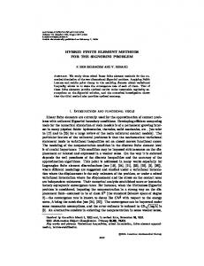
Figure 1: (a) Background mesh, with 25 nodes and 32 elements; (b) Background mesh adapted to resolve the initial condition, with 526 nodes and 900 elements. the domain , and eventually exits through x = 1. In the following, we shall let � = 7:8125 � 10 3 and T = 0:55. First, we specify the background mesh to be the 5 � 5 triangular mesh shown in Figure 1(a). This mesh is initially re ned in order to properly resolve the boundary layer along x = 0 at time t = 0, i.e. so that E0(u0; u0h ; h) = 0 (see Figure 1(b)). Numerical results are presented in Figure 2 for TOLh = 0:01 and � TOLk = 0:25. The estimated error is E (uh; h; k; f ) = 2:4742 � 10 1. In Figures 2(a), 2(b) and 2(c), 2(d) we see that the adaptive algorithm has re ned the spatial mesh in parts of the domain where the solution has a steep layer, and has kept the mesh coarse elsewhere. Figures 2(e), 2(f) show the history of the number of nodes in the spatial mesh against time, and the size of the time step against time, respectively. We note that the arti cial di�usion model introduced in [9] was used in the above experiment with C1�^ = C2�^ = 0:2 and �^max = 5:0 � 10 4.
6 Conclusions In this paper we have presented an overview of recent developments that concern the a posteriori error analysis of nite element approximations to rst-order hyperbolic problems. While for elliptic equations there is a well-established theoretical framework of a posteriori error estimation that has been successfully implemented into working adaptive algorithms (see, for example, the monograph of Ainsworth and Oden [1] for an extensive list of literature in this area), very much less is known about hyperbolic and nearly-hyperbolic problems. The main problem both from the theoretical and the practical point of view is the estimation of the stability constant of the dual problem that enters the nal error
1.4*10
4
1.2*10
4
1.0*10
4
8.0*10
3
6.0*10
3
4.0*10
3
2.0*10
3
0.0*10
0
(a)
(b)
(c)
(d) 0.03
0.025
0.02 Timestep Size
Number of Nodes
30
0.015
0.01
0.005
0.0 0.0
0.1
0.2
(e)
0.3 Time
0.4
0.5
0.6
0.0
0.1
0.2
(f)
0.3
0.4
0.5
0.6
Time
Figure 2: Layer problem for TOLh = 0:01 and TOLk = 0:25 with T = 0:55: (a) & (b) Mesh and solution (resp.) at time, t = 0:0714, with 8425 nodes and 16769 elements; (c) & (d) Mesh and solution (resp.) at nal time, t = 0:55, with 7914 nodes and 15736 elements; (e) History of nodes against time; (f) History of time step size against time.
31 bound. Current work in this area focuses on calculating the stability constant during the course of the computation, rather than using general analytical results which tend to overestimate its size by several orders of magnitude. Another important area where little progress has been made concerns the derivation of two-sided a posteriori error bounds for nite element approximations of hyperbolic problems (see, however, [17] where two-sided a posteriori bounds have been established for the locally created part of the global error). Predictably, the a posteriori error analysis of nite element and nite volume methods will be an important and fruitful area of research over the next decade; theoretical work in this eld is already making impact on large-scale engineering computations, and it is clear that this trend will continue. Indeed, guaranteed error control for the numerical solution of partial di�erential equations will be the norm rather than the exception for, to quote Babu�ska, one must have the con dence \to sign the blueprint". This article is merely a tiny scratch on the surface of a large body of theory that will, we hope, soon be unearthed.
References [1] Ainsworth, M. and Oden, J.T. (1996) A Posteriori Error Estimation in Finite Element Analysis. Series in Computational and Applied Mathematics, Elsevier. [2] Balland, P. and Suli, E. (1994). Analysis of the cell vertex scheme for hyperbolic problems with variable coe�cients. Oxford University Computing Laboratory Technical Report, NA94/01. (To appear in SIAM Journal on Numerical Analysis). [3] Bernardi, C. (1989). Optimal nite-element interpolation on curved domains. SIAM Journal on Numerical Analysis, 26, 1212-40. [4] Bank, R. (1985). PLTMG user's guide. Technical Report Edition 4, University of California, San Diego. [5] Ciarlet, P.G. (1978). The Finite Element Method for Elliptic Problems, North Holland, Amsterdam. [6] Friedrichs, K.O. (1958). Symmetric positive linear di�erential equations. Communications in Pure and Applied Mathematics, 11, 333{418. [7] Handscomb, D.C. (1995). Error of linear interpolation on a triangle. Oxford University Computing Laboratory Technical Report, NA95/09.
32 [8] Houston, P. and Suli, E. (1995). Adaptive Lagrange-Galerkin methods for unsteady convection{dominated di�usion problems. Oxford University Computing Laboratory Technical Report, NA95/24. [9] Houston, P. and Suli, E. (1996). On the design of an arti cial di�usion model for the Lagrange-Galerkin method on unstructured triangular grids. Oxford University Computing Laboratory Technical Report, NA96/07. [10] Johnson, C. (1990). Adaptive nite element methods for di�usion and convection problems. Computer Methods in Applied Mechanics and Engineering, 82, 301{22. [11] Johnson, C. (1994). A new paradigm for adaptive nite element methods. In: Whiteman, J.R., ed., The Mathematics of Finite Elements and Applications. Highlights 1993. John Wiley & Sons, 105{20. [12] Johnson, C. and Hansbo, P. (1992). Adaptive nite element methods in computational mechanics. Computer Methods in Applied Mechanics and Engineering, 101, 143{81. [13] Estep, D., Eriksson, K., Hansbo, P. and Johnson, C. (1995). Introduction to adaptive methods for di�erential equations. Acta Numerica. Cambridge University Press, 105{158. [14] Lax, P.D. and Phillips, R.S. (1960). Local boundary conditions for dissipative symmetric linear di�erential operators. Communications in Pure and Applied Mathematics, 13, 427{55. [15] Mackenzie, J., Sonar, T and Suli, E. (1994). Adaptive nite volume methods for hyperbolic problems. In: Whiteman, J.R., ed.,The Mathematics of Finite Elements and Applications. Highlights 1993. John Wiley & Sons, 289{98. [16] Mackenzie, J., Suli, E. and Warnecke, G. (1994). A posteriori error estimates for the cell-vertex nite volume method. In: Hackbusch, W. and Wittum, G., eds., Adaptive Methods: Algorithms, Theory and Applications. Vieweg, Braunschweig, 44, 221{35. [17] Mackenzie, J., Suli, E. and Warnecke, G. (1995). A posteriori error analysis of Petrov-Galerkin approximations of Friedrichs systems. Oxford University Computing Laboratory Technical Report. NA95/01. (Submitted for publication). [18] Morton, K.W. and Suli, E. (1991). Finite volume methods and their analysis. IMA Journal of Numerical Analysis, 11, 241{60.
33 [19] Morton, K.W. and Suli, E. (1994). A posteriori and a priori error analysis of nite volume methods. In: Whiteman, J.R., ed., The Mathematics of Finite Elements and Applications. Highlights 1993. John Wiley & Sons, 267{88. [20] Morton, K.W. and Suli, E. (1995). Evolution Galerkin methods and their supraconvergence. Numerische Mathematik, 71, 331{55. [21] Sonar, T. and Suli, E. (1994). A dual graph-norm re nement indicator for nite volume approximations of the Euler equations. Oxford University Computing Laboratory Technical Report, NA94/09. (Submitted for publication). [22] Suli, E. (1989). Finite volume methods on distorted meshes: stability, accuracy, adaptivity. Oxford University Computing Laboratory Technical Report, NA89/06. [23] Suli, E. (1992). The accuracy of cell vertex nite volume methods on quadrilateral meshes. Mathematics of Computation, 59, 359{82. [24] Suli, E. (1991). The accuracy of nite volume methods on distorted partitions. In: Whiteman, J.R., ed., The Mathematics of Finite Elements and Applications VII, Academic Press, London, 253{60. [25] Suli, E. (1996). A posteriori error analysis and global error control for adaptive nite element approximations of hyperbolic problems. In: Gri�ths, D.F. and Watson G.A., eds., Proceedings of the 16th International Conference on Numerical Analysis, Dundee, 1995, Pitman Research Notes in Mathematics, Longman Scienti c and Technical, Harlow.