fect of these image morphisms on the histogram has not been studied. In this work we derive the complete class of local transformations that preserve the ...
Histogram Preserving Image Transformations ∗ E. Hadjidemetriou, M. D. Grossberg, and S. K. Nayar Computer Science, Columbia University, New York, NY 10027 {stathis, mdog, nayar}@cs.columbia.edu Abstract Histograms are used to analyze and classify images. They have been found experimentally to have low sensitivity to certain types of image morphisms, for example, viewpoint changes and object deformations. However, the precise effect of these image morphisms on the histogram has not been studied. In this work we derive the complete class of local transformations that preserve the histogram or simply scale its magnitude. To achieve this the transformations are represented as solutions to families of vector fields acting on the image. It is then shown that weak perspective projection and paraperspective projection belong to this class and simply scale the histogram. The results on weak perspective projection, together with the effect of illumination, are used to compute the histogram of the projection of 3D polyhedral objects. We verify the analytical results with several examples. Moreover, we present and test a system that recognizes and approximates the poses of 3D polyhedral objects independent of viewpoint.
1. Introduction Histograms have been used widely in image analysis and recognition. Swain and Ballard in [14] used them to identify 3D objects. Currently, they are an important tool for the retrieval of images and video from databases [3] [10] [15]. Some of the reasons for their wide applicability are that they can be computed easily and fast, they achieve significant data reduction, and they are robust to local image transformations. Furthermore, color properties can be related to functionality, and must be considered for a complete recognition. Following the initial work in [14], several indexing systems [13] [4] [5] based on histograms were developed. These systems are efficient, but employ several ad–hoc assumptions. In particular, they assume that histograms are ∗ This work was supported in parts by a DARPA/ONR MURI Grant (N00014-95-1-0601), an NSF National Young Investigator Award, and a David and Lucile Packard Fellowship.
1063-6919/00 $10.00 ã 2000 IEEE
relatively insensitive to viewpoint changes and to certain object deformations[14][4]. However, the nature and properties of these transformations are not analyzed. Moreover, the viewpoint invariance does not hold for general 3D objects. On the other hand, the systems in [14] [13] are very sensitive to changes in illumination. Several proposals were made to improve robustness to these changes. In [14] the use of a supervised color constancy algorithm was suggested, which is not always practical. Later, Funt and Finlayson in [6] used histograms of edge images that can be very noise sensitive. Finally, the systems in [7] [4] use histogram moments and inter-band angles, respectively, that entail a significant loss of information. In this work we derive analytically the complete class of local image transformations that preserve the histogram or simply scale its magnitude. That is, the transformations that histogram recognition systems are insensitive to. We achieve this by modeling the image and the histogram as continuous. The transformations are represented as solutions to vector fields acting on the image. We show that divergence free fields preserve the histogram of any image. Such fields in 2D are called hamiltonian [1] [2]. Moreover, we show that fields whose divergence is constant simply scale the histogram. It is also proved that weak perspective projection and paraperspective projection of planar 2D surfaces belong to the class of transformations that scale the histogram. In fact, the scale factor depends on the tilt of the surface. Furthermore, we use the results on weak perspective projection to model histograms of 3D polyhedral objects. More precisely, we express the object histogram as the sum of the histograms of the projections of the individual faces. To account for the effect of illumination we assume that the faces are lambertian and that the dynamic range of the histogram is scaled linearly as a function of the illumination magnitude. We verify the analytical results with several examples. Further, we present a system that recognizes 3D objects independent of viewpoint and approximates their poses.
2. Modeling histograms and image transformations We assume that the image is given by an image intensity map whose domain is spatially continuous with a finite area. This intensity map, for a single color channel, is Φ: D → R1 , where D ⊂ R2 is the domain of the image. Similarly, for a color image the map is Φ: D → R3 , where R3 is a 3D color space. We assume that area in the image can be computed with the Lebesgue measure [11] on R2 . The Lebesgue measure is represented by dxdy, where x and y are the two spatial dimensions of the image. We relate the image to its histogram by a density function q. For gray–scale images the domain of q is the range of intensities. If we assume that the histogram space is also measurable, the density q that relates the two spaces becomes the Radon–Nikodym measure or derivative [11]. In other words, the image intensity map, Φ, maps the Lebesgue measure on its domain to a measure on its range. This range measure µ ∈ R is the histogram and is given by � � qΦ dr ≡ dxdy (1) µ(u) ≡ u
Φ−1 (u)
where r is a variable of intensities in the domain of density function q, u ⊂ R1 is a set of values of r, and Φ−1 (u) is the part of the image that has intensities within the range u. That is, Φ−1 (u) = {(x, y)|(x, y) ∈ R2 s.t. Φ(x, y) ∈ u}. In other words, u is a set of intensity ranges and the measure gives a real number µ(u) equal to the area of the image domain that has intensities in u. The definition of the histogram in equation (1) can be extended trivially to 3D color spaces. The domain of an image Φ can be morphed. An interesting class of deformations are the differentiable vector fields. It is possible to express such fields in terms of flow equations whose solutions [12] give rise to families of transformations. A family or path of transformations Ψt is expressed as Ψt ( x) : D → R2 , where x = (x, y) ∈ D is a point in the image, and t ∈ R is the parameter of the transformation. Transformations that arise in this manner satisfy several properties. Clearly, they are differentiable and give d back the flow relations dt Ψt = X . Further, they include the identity transformation, Ψ0 = Id, and are invertible. In this work we will only study transformations that satisfy these properties, for example rotations, scalings and other more exotic transformations we describe below. To study the effect of Ψt on the histogram we only need to study the effect of vector fields X [12].
3. Transformations that preserve the histogram We would like to find the class of transformations that preserve the histogram of any image Φ. To simplify the
1063-6919/00 $10.00 ã 2000 IEEE
analysis we break up the image into differential regions dxdy. If each differential region preserves its size under a transformation, then the histogram of the entire image is preserved and vice versa. More formally: Proposition 1 Transformations Ψt ( x) are locally area preserving if and only if they preserve the histograms of every image Φ. Proof: The histogram of image Φ transformed by Ψt is given by: � ∂Ψt ( x) � det dxdy (2) µ (u) = ∂ x −1 Φ (u) x) t (� where u is some intensity range, and det ∂Ψ∂� is the dex terminant of the jacobian of the transformation. For locally area preserving transformations the determinant is unity[2]. �Therefore, the histogram of the transformed image becomes Φ−1 (u) dxdy, which is the same as that of the original image. Hence, the histogram is preserved. Conversely, if the transformed and original images have the same histograms, then the integral in (2) must be equal to the integral in (1). Since this must be the case for any image Φ, the two integrals must have the same integrands. That is, the determinant of the jacobian of the transformation in equation (2) must be equal to one. This implies that the transformations are locally area preserving. 2 In general, a transformation, or vector field X, changes the area and the histogram of an image. Again, consider differential regions dxdy. As they flow along the streamlines of a field their sizes change. For example, if there is a “point area sink” in the image, then the areas of the differential regions decrease as they flow towards it, and area is destroyed at the “sink point”. That is, the rate of change of area per unit area, called divergence, is negative. On the other hand, if there is no “point area sink” or “point area source” in the image, the area is neither created nor destroyed. The differential regions that flow simply deform without changing their sizes. Therefore, the divergence of the field must be zero everywhere and for all t, and vice versa. Such fields are curly. More formally: d Proposition 2 Transformations Ψt with dt Ψt = X are locally area preserving if and only if divX = 0.
Proof: The proof of this theorem is given by the proof of Liouville’s theorem in [2]. 2 It is possible to generate all vector fields that satisfy proposition 2. To see this, take a function H : D → R. The gradient of H is normal to its iso–height curves. If we rotate the gradient field by 90◦ we obtain a new field which is tangent to the iso–height curves of H. This field has zero divergence. Such fields are called hamiltonian and the flow along them is called phase flow. In 2D they are given by: ΥH =
∂H ∂H i− j = J (∇H) ∂y ∂x
(3)
where i and j are the unit vectors along the x and y axes respectively, � � ∇ is the gradient, J is the antisymmetric matrix 0 1 , and H is called the hamiltonian or energy func−1 0 tion of the field. Moreover, the reverse also holds. That is, if a field preserves the histogram of an image, then the field acting on the image is hamiltonian. More formally: Proposition 3 A vector field X(twice differentiable) is divergence free if and only if it is hamiltonian. Proof: The equality of mixed partial derivatives implies that the hamiltonian field of H has zero divergence, that is div(ΥH) = 0. Conversely, if a field X = w1 i + w2 j ∂w2 1 has zero divergence, then ∂w ∂x = − ∂y and the field X has a hamiltonian function H(x, y). The hamiltonian function can be obtained by integrating either w1 or w2 . If we take �y w1 , we have H(x, y) = 0 w1 (x, y � )dy � . Both sides of this equation can be differentiated. In the result we can substi∂w2 ∂H 1 tute the condition ∂w ∂x = − ∂y to obtain w2 = − ∂x . This is the value of w2 expected by the hamiltonian field defined by equation (3). Hence, the proposition holds. 2 We have shown that histogram preserving transformations arise as solutions to a particular family of vector fields called hamiltonian. More precisely: Theorem 1 A family of transformations Ψt which arise as the solutions to a family of vector fields X preserve the histograms of all images if and only if these vector fields are hamiltonian. Proof: The proof is a direct consequence of the biconditional propositions (1)–(3). 2 Some simple examples of hamiltonian transformations are rotation, translation, shear, and stretch. An image morphed with a hamiltonian field can be transformed to give back the original one. Assume that the morphing transformation is given by Ψt , and the transformation that gives back the original is given by Ψs . The composition of the two transformations has no effect, therefore Ψs ◦ Ψt = Ψs+t = Ψ0 = Id. In turn, this implies that s + t = 0 and that Ψs , which is the inverse of Ψt , is given by Ψ−t . Further, the field whose solution gives rise to Ψ−t is given by −X, that d is dt Ψ−t = −X. There are transformations which preserve the histogram without being hamiltonian. Some examples are reflections, permutation of different areas of the image, and permutations of individual pixels[9]. However, such transformations are either not local or are discontinuous and cannot arise as solutions of flow equations. Similarly to proposition 2, transformations locally scale the area by a constant factor if and only if their divergence is also a constant. That is, we can generalize theorem 1 to get:
1063-6919/00 $10.00 ã 2000 IEEE
Theorem 2 A family of transformations Ψt which arise as the solutions to a family of vector fields X scale the histograms of all images if and only if these vector fields have constant divergence for all t. The scale factors are the determinants of the jacobians of the transformations. Proof: The proof of Liouville’s theorem[2] can be applied to images to show that the rate of change of image area as a result of vector field X is given by the integral of the divergence of the field over the domain of the image Φ. Therefore, when the divergence is a constant for all t, the change of image area is also a constant and vice–versa. We can see from equation( 1) that the histogram is linearly proportional to image area. Hence, the histogram is also simply scaled. When the divergence is a constant for all t, then the determinant of the jacobian of the transformation is also a constant [2] and can be taken out of equation( 2) to give the factor by which the histogram is scaled. Conversely, if the histogram is scaled by a constant factor for all images, then any local area in the image is scaled in size by the same factor. In turn, this implies that the rate of change of area per unit area, the divergence, is also a constant. 2 A simple family of transformations that satisfies theorem 2 are the spatial image scalings.
3.1. Examples of hamiltonian morphisms We show several examples of hamiltonian morphisms in figure 1. Each one is derived from a different energy function H. The expression gives a vector field that is applied to the image. In figure 1 (a) we show the original image and in figures 1 (b)–(g) we show six morphisms together with the energy functions they correspond to. Note that the size of the images was scaled for display purposes. As we can see the transformed images are severely deformed. However, their histograms are the same as those of the original one. Such transformations can arise in specific applications. For example figure 1 (c) may model a whirlpool, and fig. 1 (e) may model sinusoidal ripples along a matte surface. We also implemented some gradient morphisms of the test image shown in figure 1 (a). Two examples are shown in figures 1 (h)–(i). We compared the hamiltonian with the gradient field of the same function. The second column of table 1 shows the distance between the histogram of the original image and the histogram after the hamiltonian morphism. The third column shows the distance between the histogram of the original image and the histogram after the gradient morphism. We used the R, G, and B histograms. The distance between two histograms is the L1 norm of their difference divided by the number of histogram bins. Clearly, the distance due to the gradient morphism is much larger than that due to the hamiltonian one. The small errors for the case of hamiltonian morphisms are due to the spatial quantization. Note that function H was multiplied by different
(a) Original image
(b) Hamiltonian: x3
(c) Hamiltonian: (x2 + y 2 )0.7
(d) Hamiltonian: (x2 + y 2 )1.5
(e) Hamiltonian: sin (x+y)π 10
(f) Hamiltonian: sin (x+y)π sin (x−y)π 20 20
2 (g) Hamiltonian: (sin (x+y)π 20 )
(h) Gradient of: sin (x+y)π sin (x−y)π 20 20
(i) Gradient of: (x2 + y 2 )1.5
Figure 1. In (a) we show the original test image. In (b)–(g) we show six hamiltonian morphisms of this image together with the energy functions they correspond to. All hamiltonian morphisms have the same histogram as that of the original image, up to spatial quantization error. In (h)–(i) we show two gradient morphisms of the original image shown in (a). The gradient morphisms have a different histogram both from the histogram of the original image and those of the hamiltonian morphisms. The actual distances between the histograms of these morphed images and the original image in (a) are shown in table 1. Note that the origin of the coordinate frame is the geometrical center of the original image, the x axis is horizontal, and the y axis is vertical.
1063-6919/00 $10.00 ã 2000 IEEE
Function x3 (x2 + y 2 )0.7 (x2 + y 2 ) (x2 + y 2 )1.5 sin (x+y)π 10 2 (sin (x+y)π 20 ) (x+y)π sin 20 sin (x−y)π 20
Hamiltonian 0.488 1.870 1.302 2.820 1.003 1.083 3.901
Gradient 16.763 121.000 265.641 42.609 12.182 11.188 34.049
Table 1.
Effects of the hamiltonian and gradient morphisms on the histogram. The second column shows the distance of the histogram of the hamiltonian morphism from the histogram of the original image shown in figure 1 (a). The third column shows the distance of the histogram of the gradient morphism from the histogram of the same original image. The distance is the L1 norm of the difference histogram divided by the number of histogram bins.
constant factors for each morphism in order to restrict the size of the transformed images.
4. Applications of hamiltonian fields We study the effect of some projection models on the histogram. Clearly, perspective projection does not preserve the histogram. However, we will use the two theorems presented previously to show that weak perspective projection and paraperspective projection simply scale the histogram. Finally, this result will be used to justify a recognition system that can identify and approximate the pose of 3D polyhedral objects.
4.1. Histograms under weak perspective projection Consider a planar patch, with some texture on it, in a space equipped with an x ˆyˆzˆ coordinate frame. The weak perspective projection of this patch is shown in figure 2 (a). The first stage of this projection is the orthographic projection which can be done either frontally or under some arbitrary tilt φ. The effect of a tilt is to both shear and scale the frontal orthographic projection. The shearing is a hamiltonian transformation. According to theorem 1 it does not affect the histogram of the image. However, the scaling does alter the histogram. In particular, according to theorem 2, it scales it by the determinant of the jacobian of the transformation, which is cos φ. The image is then mapped from the projection plane to the image plane. This mapping is a uniform scaling and the 2 determinant of its jacobian is fz2 , where f is the focal length and z is the distance of the object from the origin of the
1063-6919/00 $10.00 ã 2000 IEEE
coordinate system. According to theorem 2 this is also the scale factor of the histogram. The weak perspective projection consists of the concatenation of the orthographic projection and the mapping on the image plane. The product of the scaling factors of the two stages is given by f 2 cos φ , z2
(4)
which is the overall scaling factor of the histogram in weak perspective projection.
4.2. Histogram under paraperspective projection The paraperspective projection of a planar patch is shown in figure 2 (b). It first undergoes parallel projection with a skew angle α. Similarly to weak perspective projection, the determinant of the jacobian of the projection transformation is proportional to the cosine of the tilt of the object. However, in parallel projection the projection axis is skewed. Therefore, the relative tilt of the object is (φ − α). Moreover, the size of the projected image increases as a result of the skew angle by a factor inversely proportional to cos α. That is, the determinant of the jacobian of the parallel projection transformation is cos(φ−α) cos α . According to theorem 2 the histogram is scaled by this factor. To complete the projection we map from the projection plane to the image plane. Similarly to weak perspective pro2 jection, this mapping scales the histogram by fz2 . The overall scaling of the histogram is equal to the product of the 2 two scale factors and is given by fz2 cos1 α cos(φ − α). Note that paraperspective projection reduces to weak perspective projection when the angle with the optical axis, α, is zero. In practice, the histogram of a projection is also affected by illumination. In our work we assume that the spectral composition of illumination is always the same and that only the intensity changes. We also assume that its effect is to linearly scale the dynamic range of the histogram.
4.3. Histograms of polyhedral objects under weak perspective projection We compute the histogram of matte polyhedral objects in terms of the histograms of their faces. We actually consider the frontal histograms, Bi for each face i, under a normalized illumination scaling factor. To account for the orientation of the faces we use a coordinate frame centered on the object. In this frame take the polar angle of the normal to the ith face to be φi and the azimuth angle to be θi . Similarly, the polar angle of the unit vector towards the camera is taken to be φc , and the azimuth angle is taken to be θc . The dot product between the camera unit vector and the normal to the ith face gives cos ηi =
Figure 3. Arbitrary poses of the four objects on which the recognition system was tested. Projection Plane
^ x
π/2 − φ
n Planar Patch
Image Plane
We assume that the projections of the individual faces follow the weak perspective model. Therefore, the magnitude of the histogram of each visible face i is scaled by the 2 ηi multiplicative factor f cos that is given by equation (4). z2 In addition, the tilt of each face alters the illumination conditions and scales the dynamic range of the histogram by a factor li . Therefore the histogram of the object is given by:
f z
^ z
Bobj (j) =
^ y
(a) Projection Plane
π/2 − φ
n
n f2 � max(cos ηi , 0)Bi (jli ) z 2 i=1
(5)
where j is the histogram bin, i is the face number, and n the total number of faces. Note that when cos ηi < 0 the ith face is not visible and its histogram does not contribute to the object histogram.
^ x Planar Patch Image Plane
f
α
^ z
z
^ y
(b)
Figure 2. The figure in (a) is the geometry of weak perspective projection. A planar patch is projected under a tilt angle φ. The figure in (b) is the geometry of paraperspective projection. The skew angle of the parallel projection is α, and the tilt of the object is φ.
sin φi sin φc cos(θi + θc ) + cos φi cos φc , where ηi is the tilt of face i with respect to the camera viewpoint.
1063-6919/00 $10.00 ã 2000 IEEE
4.4. Recognition of polyhedral objects We implemented a system that uses the R, G, and B histograms to recognize matte rectangular parallelepipeds. It assumes that the histogram is given by equation (5), and computes in advance the frontal histograms, Bi ’s, of the faces of all objects. Furthermore, it stores the polar and azimuth angle of all faces with respect to coordinate frames centered on the objects. The input to the system is the histogram of the test object. To compute it the object is segmented manually from the background. The system estimates the histogram of each database object sequentially and computes its match error compared to the input histogram. The test object is identified as the database object that has the minimum match error. As can be seen from equation (5) the histogram of an object depends on 6 parameters; namely the angles φc and 2 θc , the global parameter g = fz2 , and the illumination scaling li for each of the visible faces, i = 1, 2, 3. The range of the scale parameter g was 50% − 200%, and the range of all illumination scale factors li was 60% − 135%. Note that
Object 1 2 3 4 Total
Tests 10 14 9 7 40
Rank=1 10 12 9 7 38
Rank=2 0 2 0 0 2
Table 2.
Recognition results for 4 objects in the horizontal order shown in figure 3. In the second column we show the number of test poses per object. In the third column we show the number of these object instances that are correctly recognized, and in the last column the number of object instances ranked second.
φc and θc are essentially the pose of the object. The match error of an object is given by the L1 norm of the difference between the input histogram and the histogram of the object. More precisely, the match error is given by: ME = g
3 � 256 � c=1 j=1
c |Bin (j)
−
n �
max(cos ηi , 0)Bic (jli )|
i=1
(6) where Bin is the histogram of the input object, c is the color channel and 256 is the number of color histogram bins. This function was minimized with the direct search complex optimization algorithm of the IMSL [8] library. We used several different initial conditions to avoid local minima. The system can recognize objects under arbitrary poses, even if different poses and faces have completely different histograms. We tested the algorithm with a total of 40 poses of 4 objects. The poses were selected arbitrarily. Eight of these poses are shown in figure 3. In table 2 we show the recognition results. In the second column of the table we show the number of test poses per object. In the third column we show the number of object poses correctly found to be the first match to the test case, and in the last column the number of poses found to be the second match. In the two erroneous classifications the object shown second horizontally in figure 3 is identified as the first object of the same figure. This is because both objects have faces with very similar colors. The performance of the algorithm improves when the different faces have “dissimilar”, or orthogonal, histograms. In this case the pose estimation of the object becomes more precise. Such an example is the first object in the second row of figure 3 where pose is estimated within 7◦ .
4.5. Summary In this work we derived the complete class of local image transformations that preserve or scale the histogram. In other words, the transformations that histogram recognition
1063-6919/00 $10.00 ã 2000 IEEE
systems are insensitive to. To achieve this, we first assumed that the image is spatially continuous and defined a density measure over it that gave the histogram. We then showed that weak perspective projection and paraperspective projection scale the histogram. Finally, a system was presented that identified 3D orthogonal parallelepipeds. We plan to generalize our results to model some types of elastic deformations.
References [1] R. Abraham and J. Marsden. Foundations of mechanics. Benjamin/Cummings Publ. Co., 1978. [2] V. Arnold. Mathematical Methods of Classical Mechanics. Springer-Verlag, 1989. [3] J. Bach, C. Fuler, A. Gupta, A. Hampapur, B. Horowitz, R. Humphrey, R. Jain, and C. Shu. The virage image search engine: An open framework for image management. In In SPIE Conference on Storage and Retrieval for Image and Video Databases IV, volume 2670, pages 76–87, March 1996. [4] G. F. S. Chatterjee and B. Funt. Color angular indexing. In Proceedings of the 4th European Conference in Computer Vision, volume 2, pages 16–27, Berlin, Germany, 1996. [5] S. Cohen and L. Guibas. The earth mover’s distance under transformation sets. In Proceedings of the 7th International Conference on Computer Vision, Kerkyra, Greece, September 1999. [6] B. Funt and G. Finlayson. Color constant color indexing. IEEE Transactions on Pattern Analysis and Machine Intelligence, 17(5):522–529, May 1995. [7] G. Healey and D. Slater. Global color constancy: Recognition of objects by use of illumination-invariant properties of color distributions. J. Opt. Soc. Am. A, 11(11):3003–3010, November 1994. [8] I. Inc. User’s Manual MATH/Library. Texas: IMSL Inc., 1991. [9] J. Koenderink and A. J. V. Doorn. The structure of locally orderless images. International Journal of Computer Vision, 31(2–3):159–168, 1999. [10] W. Niblack. The QBIC project: Querying images by content using color, texture, and shape. In In SPIE Conference on Storage and Retrieval for Image and Video Databases, volume 1908, pages 173–187, April 1993. [11] H. L. Royden. Real Analysis. MACMILLAN, 1968. [12] M. Spivak. Calculus on Manifolds. Benjamin/Cummings, 1965. [13] M. Stricker and M. Orengo. Similarity of color images. In In SPIE Conference on Storage and Retrieval for Image and Video Databases III, volume 2420, pages 381–392, Feb. 1995. [14] M. Swain and D. Ballard. Color indexing. International Journal of Computer Vision, 7(1):11–32, 1991. [15] H. Zhang, C. Low, W. Smoliar, and J. Wu. Video parsing, retrieval and browsing: An integrated and content–based solution. ACM Multimedia, pages 15–24, 1995.