I. INTRODUCTION
CW Interference Effects on Tracking Performance of GNSS Receivers JAEGYU JANG MATTEO PAONNI BERND EISSFELLER Institute of Geodesy and Navigation University of Federal Armed Forces Munich
Analytical expressions are suggested for GNSS receiver performance such as the effective C=N0 , code tracking (DLL) error and carrier phase tracking (PLL) error for a receiver affected by CW interference signals. The navigation signal model is applied to GNSS power spectral density (PSD) to interpret spectral line effects within receiver tracking low pass filter, limited by navigation data bits. A scaled envelope model is also introduced to estimate average susceptibility of signal against CW interferences. Numerical results show how the spectral lines and correlator model can affect the tracking performances, and the sensitivity of GNSS signals against the CW interferer is investigated by varying data bit duration or integration time.
Manuscript received June 22, 2009; revised March 1and August 25, 2010; released for publication November 11, 2010. IEEE Log No. T-AES/48/1/943611. Refereeing of this contribution was handled by S. Pullen. Authors’ address: Institute of Geodesy and Navigation, University of FAF, Aerospace Engineering, Werner-Heisenberg-Weg 39, Neubiberg, Bavaria 85577, Germany, E-mail: (
[email protected]).
c 2012 IEEE 0018-9251/12/$26.00 °
Vulnerability of GNSS signals to intentional or unintentional interference signals is one of the major issues of many applications, because satellite navigation signal has a very low power, e.g. ¡155—¡160 dBW, a value that is under the noise floor level. Pulsed signal interference such as DME/TACAN on L5-band is an already well-known unintentional source [1, 2]. An emitter of 1 W, which can be implemented in very small handsets, can already jam most of the civil GPS receivers within a distance of 30 Km or even more around the location of this jammer. E6-band of Galileo can be potentially affected by European Amateur TV or HARM signals because E6 is not a protected Aeronautical Radio Navigation Service (ARNS) band. So, investigations about the different types of interferences and techniques to mitigate their effects on a GNSS receiver are highly important issues to protect users from those unintentional/intentional RF signals. On the one hand, intensive investigations to mitigate interferences have been conducted by many authors during the past years, including frequency domain techniques [3], time domain techniques [4, 5], time-frequency domain techniques [6], and array antennas [7, 8, 9]. On the other hand investigations to analyze effects of interference on GNSS signals have been performed. References [10, 11] suggest an analytical model to interpret the postcorrelation effects of RF interferences (RFI), resulting in very useful mathematical expressions for the effective C=N0 , the code tracking error and the carrier tracking error. Because the model in [10], [11] assumes continuous spectrum density functions to analyze partialband or narrowband interferences, there is a limitation to interpret the effects of CW type signals. Since the spectrum of a GNSS signal can be expressed as a train of impulse functions due to its short and repeating pseudorandom code sequence, approaches to interpret its effects was limited to specific situations such as an in-phase status or a coincidence with spectral line [12, 13]. Recently, fortunately, investigations regarding spectral lines of GNSS signal have been conducted in detail. CW effects on C=N0 are investigated in several theoretical and experimental works [14—16] and effects on the carrier tracking at spectral lines are shown briefly in [17]. However they are based on the integrate-dump model of GNSS with a CW signal and their approaches have limitations to be enhanced by looking for carrier or code tracking closed-form models such as the formulations given in [10], [11]. In this paper we applied the navigation signal model [18] into representative performance measures to analyze GNSS receiver tracking performances
IEEE TRANSACTIONS ON AEROSPACE AND ELECTRONIC SYSTEMS VOL. 48, NO. 1
JANUARY 2012
243
when CW interferences are present. The effective C=N0 , the code tracking thermal noise and the carrier tracking thermal noise, are considered as the measures. Based on the navigation signal model, analytical models for the performance measures are derived. Due to the continuous spectrum-like shape of the introduced model, spectral line effects of the GNSS signal spectrum could be easily integrated with the postcorrelation models suggested by [10], [11], and [13]. As will be clearer later, this model is more straightforward and easier to be applied than the classical approach based on the integrate-dump filter, while at the same time the derived effective C=N0 model is shown to be accurate as the model based on the integrate-dump filter introduced in [17], [15]. Numerical results regarding tracking performance well interpreting the effect of spectral line and low pass filter of the tracking loop are also presented. It is explained that the worst code tracking error results from the combination of the worst spectral line and the early-minus correlator spacing, while the overall pattern of errors coinciding with spectral lines is shown following the theory of [10], [13]. A scaled envelope model to interpret average effects neglecting the characteristics of individual pseudorandom noise (PRN) code caused by the cross-correlation property of the Gold code is also suggested. Such a model can be helpful to overcome a limitation of the conventional jamming margin based on CW susceptibility estimation [19]. Finally we analyze effects of integration duration time onto the performance measures, and the results that are presented here clearly show that a short integration time is helpful in order to reduce the sensitivity of GNSS signals to CW interferences. II. EFFECTS OF FINITE-LENGTH CODES TO GNSS DSSS SPECTRUM Assuming random sequences, the normalized autocorrelation function (AF) and the power spectral density (PSD) of a direct sequence spread spectrum (DSSS) signal assume the well-known triangular form in (1) and the sinc-function form in (2), respectively: 8 < 1 ¡ j¿ j for j¿ j · Tc Tc (1) R(¿ ) = : 0 elsewhere Z 1 R(¿ )e¡j2¼¢f¿ d¿ = Tc sinc2 (fTc ) (2) Gs (f) = ¡1
where ¿ is the code delay in chip, Tc is the chip duration in seconds, f is the frequency in Hz and sinc(x) = sin(¼x)=¼x. Rectangular chips with a perfectly random binary code are assumed in the equations above. In reality GNSS employs periodical codes with a period sufficiently long to let them appear random 244
(hence their name of pseudorandom sequences). The simplest pseudorandom sequences are the maximum-length pseudonoise (PN) code sequences (or m-sequences) with a finite length that repeats every N bits. Due to the repeatability, GNSS signals have a periodical AF and its period is equal to the m-sequence period NTc , where N is the sequence length in chips. Since in an m-sequence the number of negative values is always larger than the number of positive values, the normalized AF has a DC term that equals ¡1=N outside of the correlation interval. Thus the periodic (normalized) AF of the finite sequence can be expressed as the sum of the DC term and an infinite series of the triangle function R(¿ ) as it can be seen in (3) 1 X ¡1 N + 1 ±(¿ + nNTc ) (3) + R(¿ ) − RPN (¿ ) = N N n=¡1 n6=0
where ± is the Dirac delta function and − is the convolution operator. Applying FFT (fast Fourier transform) to (3) above as done in (2), we can derive the PSD of the finite sequence as follows: GPN (f) =
1 ±(f) N2 +
¶ 1 ³ ´ μ N +1 X n 2 n sinc : ± f + N 2 n=¡1 N NTc n6=0
(4) The PSD equation (4) is composed of a train of impulse functions and its average envelope can be expressed as follows: GENV (f) =
N +1 sinc2 (fTc ): N2
(5)
The envelope function in (5) has the same shape of the one expressed in (2) except for the scale factor Tc . The Gold code used in GNSS has slightly different characteristics. As examples, the AF and the PSD of an arbitrary Gold code are plotted in Fig. 1 and Fig. 2. It must be noted that the spectral lines in Fig. 2 have been represented to have an interval of 250 kHz in order to make the figure readable, while the real GPS spectral lines have 1 kHz intervals. Normally effects of partial narrowband interferences such as FM signals or wideband interferences such as DTV signals can be analyzed with the PSD of random sequence in Fig. 2 or with (2), although the PSD of GNSS signals is composed of spectral lines as can be seen in Fig. 2. If the bandwidth (BW) of the interference is wide enough (e.g. BW > 100 kHz), spectral lines covered by the interference BW are averaged to the smooth spectrum level assuming correlation process and we can assume the PSD of GNSS signals as the one in (2) use the partial band interference theory.
IEEE TRANSACTIONS ON AEROSPACE AND ELECTRONIC SYSTEMS VOL. 48, NO. 1
JANUARY 2012
Fig. 2. PSD comparison between random sequence and Gold code.
Fig. 1. Normalized AF of Gold code (N = 1023).
However the spectral lines of GNSS signals make the interference analysis difficult in the case of very narrowband interferences such as a CW signal. On one side the CW interference attenuates receiver performance only when the frequency of the interferer is near a spectral line and the difference between the spectral lines’ frequencies and of the narrowband interferer is falling within low pass filter bandwidth of the tracking loop. Assuming 20 ms coherent integration time or 50 Hz loop filter bandwidth, 10% of Doppler frequencies are affected by CW interferences. In other words, a static in-band interference source cannot jam GNSS signals over 90% of time, without considering hardware (H/W) effects on the quantization stage. On the other side every PRN code has a unique spectral line pattern and this implies that the worst case spectral line or interference level of specific frequencies should be estimated or measured case by case. The worst case spectral line power
S(k) =
8 > > > > > > > > > > > > > > > > > > > > > > > >
k > > ¼ > > N > > > > > > μ ¶0 μ ¶ 12 > > > ¼ k k > 2 2 > sin ¼ sin > > N B 2m N C > > B μ ¶ C > 4 μ ¶ > 2 @ A , m even, > ¼ k > k : cos ¼ N
would be below only 18.3 to 21.5 dB w.r.t. the total code power depending on PRN code of GPS C/A signal, while typical values are near or below 30 dB.
mN
or
μ
k ¼ N
μ
k ¼ N
2
cos or 4 μ
¶2 tan2
μ
k ¼ N
k ¼ N
¶2
¶0 B B @
μ
¼ k mN
sin
2
μ
cos
, m odd
(7)
¼ k 2m N
μ
for sine-BOC
¶ 12
C ¶ C A , m odd ¼ k
for cosine-BOC
mN
JANG, ET AL.: CW INTERFERENCE EFFECTS ON TRACKING PERFORMANCE OF GNSS RECEIVERS
245
Fig. 3. Spectral lines and envelope of GPS L1 C/A PRN6 code.
Fig. 4. Power difference between envelope PSD of m-sequence and PSD of GPS C/A PRN6 (BW = 40 MHz).
where m = Tc =Ts is the BOC modulation index with Ts defined as the half-period of a square wave generated with subchip frequency fs . The PSD of the navigation data can be assumed as a random code stream without repeatability and can be expressed as (8) assuming data duration time of Td (À Tc ). (8) Gd (f) = Td sinc2 (fTd ): We can derive an analytical form of the PSD of navigation data modulated GNSS DSSS signal as (9) using the convolution property of the Dirac delta function. 1 X sinc2 ((f ¡ k ¢ ¢f) ¢ Td ) ¢ jC(k)j2 ¢ S(k) GNav (f) = Td k=¡1
(9) where C(k) = Cprn (k)=N is the normalized DFT of code sequence. The navigation signal model-based PSD defined as (9) is very useful to analyze interference effects to DSSS signals with finite 246
Fig. 5. Enlarged spectral lines of PSD in Fig. 3 and PSD of data modulated signal.
pseudorandom code as can be seen in [18], [20]. We expect that applying this navigation signal model to the conventional partial band interference theory makes it easier to analyize CW interferences from a spectral point of view. In the case of pilot signal, Td can be substituted by the coherent integration time Tcoh for the CW interfenece analysis, because the observation window of duration Tcoh plays the role of the data with the same duration. We plotted the PSD of GPS C/A PRN 6 code in Fig. 3 with the PSD of the envelope model of (5). Due to the property of Gold code spectral lines it results in a difference with respect to the envelope line of m-sequences. The difference computed as the envelope minus the PSD of the PRN code is represented as a histogram in Fig. 4 with a normal distribution fit line. The two-sided BW of 40 MHz and the ideal rectangular bandpass filter have been assumed to get the histogram. The rms value of the difference of the PRN 6 code is approximately 6.37 dB and the maximum difference of 30 dB locates at zero Doppler line corresponding to the DC component explained in (4). This difference can be used as a figure of merit (FOM) to indicate the weakness of the Gold code against narrow bandwidth interferences or CW interferences at specific Doppler frequencies. The excess line weight (ELW) defined in [20] is a representative example of the FOM to describe an increase of the sensitivity against CW signals or narrowband signals which are sent on these particular frequencies. Applying the navigation data message into the PSD of Fig. 3 we can get the PSD model of the navigation signal model like Fig. 5. We focused on the worst case line component frequency of 227 kHz of the PRN code 6. The PSD of a data modulated signal can be displayed as a train of sinc functions. Each sinc function is centered at the spectral line
IEEE TRANSACTIONS ON AEROSPACE AND ELECTRONIC SYSTEMS VOL. 48, NO. 1
JANUARY 2012
position with a scaled amplitude equal to the duration time Td . Now we can assume the PSD of Gold code as continuous spectral density shape of which the envelope is the PSD of random codes in (2).
derived in (9) into the denominator of the spread spectrum gain adjustment factor of (11), the effective C=N0 affected by CW interference can be obtained as follows:
IV. INTERFERENCE EFFECTS TO USER EQUIPMENT
(C=N0 )eff
RFI affects the tracking loop performance of user equipment and the effects can be generally measured by FOMs such as the effective CS =N0 and tracking performance of delay lock loop (DLL) or phase lock loop (PLL). In this section we introduce the FOMs based on continuous spectrum and apply the PSD based on the navigation signal model described in the previous section for the CW interference interpretation. In [13], [11] the effective Cs =N0 is defined as (10) that is accounting for the effects of both RFI and white noise. (CS =N0 )eff =
1
(10)
C =C 1 + i S (CS =N0 ) QRC
where CS =N0 is the carrier-to-noise-power ratio without any interference [dB], Ci =CS is the interference-to-received-signal power ratio [dB], Rc is the chipping rate of the desired signal [chip/s] and Q is the spread spectrum gain adjustment factor [dimensionless] defined as follows: R1 jH (f)j2 GS (f)df R 1¡1 R (11) Q= RC ¡1 jHR (f)j2 Gi (f)GS (f)df
2 ¾DP,' = BL (1 ¡ BL Td )
R B=2
CS R B=2 G (f)df N0 ¡B=2 S =R C B=2 G (f)df + i Td sinc2 ((fi ¡ k¢f) ¢ Td )jC(k)j2 S(k) ¡B=2 S N0
(12) where B is the effective bandwidth of the receiver transfer function HR (f) which is assumed as a brick-wall filter here, and fi is the interference frequency offset relatively to zero Doppler frequency of GNSS signals in Hz. Note that the kth spectral line is the nearest one to fi and that the coherent integration time is limited to data bit duration time Td . Assuming infinite bandwidth, (12) derived above is equivalent to the mathematical C=N0 expression defined and verified by experiments in [15] neglecting its tracking error effects. To investigate the carrier phase tracking performance due to CW interference, we derived the theoretical PLL noise thermal noise model affected by partial band interferences. We assumed the dot-product (DP) discriminator for the tracking loop model. Derivation of the equation can be found in Appendix I and the tracking variance equation in rad2 is formulated as follows:
0 1 R B=2 Ci R B=2 Ci R B=2 G (f)G (f)df G (f)df + G (f)G (f)df S S ¡B=2 S B C N0 ¡B=2 i N0 ¡B=2 i B1 + C ´ ´ ³ ³ @ A 2 2 R R CS CS B=2 B=2 G (f)df 2T G (f)df S d S ¡B=2 ¡B=2 N0 N0
¡B=2 GS (f)df +
(13) where HR (f) is the receiver transfer function, GS (f) and Gi (f) are, respectively, the PSD for the desired and the interfering signals, both normalized to unit area over infinite bandwidth. Substituting the PSD
R B=2
where BL is the loop bandwidth in Hz and Td is integration duration time in seconds. Substituting the PSD derived in (9) into (13), the variance can be redefined as follows:
Ci Td sinc2 ((fi ¡ k¢f)Td )jC(k)j2 S(k) N 2 0 ¾DP,' = BL (1 ¡ 0:5BL Td ) ´2 CS ³R B=2 G (f)df N0 ¡B=2 S 1 0 R B=2 Ci 2 2 G (f)df + T sinc ((f ¡ k¢f)T )jC(k)j S(k) i d ¡B=2 S C B N0 d C: £B 1 + ³ ´ A @ 2 CS R B=2 2Td GS (f)df ¡B=2 N0 ¡B=2 GS (f)df
+
JANG, ET AL.: CW INTERFERENCE EFFECTS ON TRACKING PERFORMANCE OF GNSS RECEIVERS
(14)
247
The code tracking thermal noise of the noncoherent DP power (DPP) discriminator has been also derived in a similar way (Appendix II) in sec2 and can be expressed as (15) applying (9).
2 ¾DPP,¿
μ R B=2
Ci 2 2 ¡B=2 GS (f) sin (¼fi D)df + N Td sinc ((fi ¡ k¢f)Td )jC(k)j S(k) sin(¼fi D) 0 = BL (1 ¡ 0:5BL Td ) ´´2 CS ³ ³R B=2 2¼ ¡B=2 fi GS (f) sin2 (¼fi D)df N0 · ¸ 10 52 £ 1 ¡ ª + 7ª 2 + ª 3 3 15 2
with R B=2
C G (f)df + i Td sinc2 ((fi ¡ k¢f)Td )jC(k)j2 S(k) ¡B=2 S N0 ª= ´2 CS ³R B=2 Td GS (f)df ¡B=2 N0
(16) where D is the early-minus-late (EML) spacing in seconds. For other types of discriminators the mathematical models provided in [10] for the coherent/noncoherent EML and in [21] for the DP, respectively, can be used instead of (13) to apply the navigation signal model. From the equations derived above we can apply specific spectral line effects due to CW interference to generate closed forms that are based on continuous spectrum Gs . In the case of infinite bandwidth or wide enough transmission bandwidth, we can, for simplicity, assume the normalized GNSS signal power integral as unity as follows: Z
B=2
¡B=2
Gs (f)df =
Z
B=2
¡B=2
Tc sinc2 (f ¢ Tc )df ¼ 1: (17)
V. NUMERICAL RESULTS For numerical results, GPS C/A code PRN 6 has been used and its worst line component has power of nearly ¡22:29 dB at 227 kHz frequency with respect to center frequency. The worst line amplitude of GPS satellite codes (PRN 1 to 32) varies from ¡23:78 to ¡21:26 dB [13] so the choice of PRN 6 seems to represent well the average effects. We considered a GPS C/A receiver with effective thermal noise density of N0 = ¡203 dBW/Hz without implementation losses and received signal power of Cs = ¡158 dBW, for a nominal received C=N0 of 45 dB-Hz. CW with power of Ci = ¡150 dBW has been assumed as an interference source, corresponding to jamming-to-signal power ratio of 8 dB. For all the results represented from Fig. 6 to Fig. 12 a coherent 248
integration time Td of 20 ms has been considered, being Td limited by the navigation data bit duration. In Fig. 6 effective C=N0 is represented by varying Doppler frequencies from 225 kHz to 229 kHz to
(15)
focus on the worst case line component at 227 kHz. In the C=N0 graph we can see that the receiver performance is affected severely when the CW interference signal coincides with spectral lines, e.g. deep troughs of C=N0 with distance 1 kHz. As expected, a direct relationship between the spectral line amplitudes deduced from the Fourier transform characteristics of a C/A PRN code and C=N0 degradations can be figured out in Fig. 5. By applying the navigation signal model, the troughs of the C=N0 have sinc-like shapes of which null-to-null space is determined by the navigation data bit duration Td (or integration duration time Ti , if Ti < Td ). Approaching by the correlation process model described in [16], these characteristics come from sinc-function shape at CW signal outputs of the integrate-and-dump (I&D) filters. As mentioned in Section II, only 10% of Doppler frequencies of a jammer can pass through the tracking filter assuming 20 ms integration duration time, e.g. sinc-like troughs in Fig. 6. The left 90% frequency area is out of our concern because it is not affected notably. The effective C=N0 at spectral lines (or peak effective C=N0 ) of mainlobe and first sidelobes is shown in Fig. 7 to see the worst case attenuations within pass band (from ¡2 MHz to 2 MHz here). The scaled envelope line denoted in bright color is calculated using the envelope spectrum expressed by (5) scaled by data bit duration to reflect the effect of the navigation signal model. The envelope PSD corresponds to m-sequence of which the only cross-correlation value outside the triangular AF is a DC-term. Therefore it can represent an average effect neglecting the Fourier transform characteristics of each PRN code. We can see that the average effect follows the shape of GNSS sinc-function spectrum and can be interpreted as the prompt-correlator used to estimate C=N0 in the receiver [23]. The C=N0 line labeled as random codes, computed by (2), does not attenuate compared with other models (see Fig. 7). Actually applying continuous PSD Gs (f) to CW Dirac delta function is a miss-interpretation about the partial band theory suggested by [11].
IEEE TRANSACTIONS ON AEROSPACE AND ELECTRONIC SYSTEMS VOL. 48, NO. 1
JANUARY 2012
Fig. 6. Effective C=N0 caused by CW interference versus Doppler frequency.
Fig. 7. Effective C=N0 at spectral line positions.
We showed the carrier phase tracking thermal noise and the code tracking thermal noise near the worst spectral line in Fig. 8 and in Fig. 9. The EML chip spacing is assumed as 0.5 chips (or 488.76 ns) for the DPP discriminator. Loop bandwidth of the code and carrier tracking loops are 5 Hz and 20 Hz, respectively. The attenuation of performance for both code and carrier tracking loops has similar characteristics to that obtained for the effective C=N0 except for the attenuations at the sidelobes of the sinc-functions that are suppressed in some degree. This can be interpreted considering that the performance of tracking degrades more slowly in high C=N0 conditions than in low C=N0 in conventional white Gaussian noise theory [13]. In Fig. 10 and Fig. 11 peak tracking noise error at spectral lines within pass band are shown in order
Fig. 8. Carrier phase tracking thermal noise versus Doppler frequency.
Fig. 9. Code tracking thermal noise versus Doppler frequency.
to compare performances of code and carrier tracking loops under CW interferences. As already performed in Fig. 7, we represented both the random code line and scaled envelope line together in order to have a fair comparison. Overall tracking error patterns in Fig. 10 and Fig. 11 follow the properties of the correlator type used in the receiver, which is described in [23], [10]. The average carrier tracking error denoted by the scaled envelope line has a similar pattern to the effective C=N0 in Fig. 7 because the tracking loop depends only on the prompt-correlators. However the average code tracking error has its maximum error at different Doppler frequency locations due to usage of the EML correlators. The worst tracking performance of each PRN code occurs at different frequency locations (although the same type of discriminator is used) because the Fourier transform
JANG, ET AL.: CW INTERFERENCE EFFECTS ON TRACKING PERFORMANCE OF GNSS RECEIVERS
249
Fig. 10. Carrier tracking thermal noise at spectral line positions.
Fig. 12. CDF of code tracking noise denoted in Fig. 11.
Fig. 13. Integration duration time versus PSD. Fig. 11. Code tracking thermal noise at spectral line positions.
characteristics of each Gold code is different. In the case of code tracking of C/A PRN6 represented in Fig. 11, the worst carrier tracking error occurs at Doppler frequency of 346 kHz while the worst error of continuous spectrum models occurs around 471 kHz. The code tracking error at the worst spectral line of 227 kHz showed the 3rd worst error. These facts mean that the worst performance in the code tracking does follow neither the correlator model nor the worst spectral line independently when a CW interference is present, but it shows combined effects due to both of them. In Fig. 12 we plotted the cumulative density function (cdf) of the code tracking error of Fig. 11. Peak code tracking error at spectral lines is considered and the occurrence probability between 1¾ and 3¾ is shown. The worst tracking errors with 2¾ are close to 2 m. Considering nominal tracking error of nearby 1.8 m, we can know 95% of peak 250
errors experience 20 cm tracking error increase respectively. Considering the entire region without line components, only the Doppler frequency area of almost 0.5% is severely affected by CW signals in the case of static interference sources. However we have to consider the peak errors for swiping sources corresponding to possible intentional jammers. Finally numerical results varying integration duration time are also presented. As already said, the maximum integration time is limited by the bit duration time of 20 ms and the minimum integration time is limited by the C/A code sequence length of 1 ms. In Fig. 13 the PSD of the navigation signal model is plotted as well as the PSD of random codes computed by (2). By reducing integration time (that corresponds to a faster data rate) the PSD becomes closer to the continuous PSD that is obtained in the case of random codes, which is already well described in [18]. It must be noted that the signal power coinciding with the spectral lines decreases
IEEE TRANSACTIONS ON AEROSPACE AND ELECTRONIC SYSTEMS VOL. 48, NO. 1
JANUARY 2012
Fig. 14. Integration duration time versus effective C=N0 .
with an inversely proportional relation with respect to the integration time, and this affects directly the performance of the receiver, as can be seen in Fig. 14 and Fig. 15. By reducing the integration time, the spectral spread of the sinc function replacing each spectral line becomes wider and as a consequence the interval of Doppler frequencies affected by CW interference increases. As shown in the figures, when the coherent integration time is 1 ms the entire region is affected. On the other side when the coherent integration time is reduced, the worst case error is also reduced and therefore it can be said that the sensitivity to CW interferences is lowered by reducing the integration time. This conclusion goes exactly in the opposite direction of the common concept of increasing the integration time to increase the robustness of the receivers against interferences. However, considering the ELW used in the spreading code selection criteria of Galileo, as explained in [20], this can be understood as an acceptable characteristic of a DSSS exposed to CW interferences VI. CONCLUSION In this paper we have applied the navigation signal model, which was originally suggested to investigate the spectral separation coefficient (SSC) of GNSS signals modulated by navigation data messages, to a new context by using this model to analyze the impact of CW interferences on GNSS signal and receiver performance. By using continuous GNSS spectrum including spectral line properties and considering the I&D filter effects, we have formulated analytical equations representing the effective C=N0 , DLL error, and PLL error when a CW interference is present. Such a spectrum approach is easy to apply in order to analyze the effects of specific types of jammers on the receiver tracking loop model with the analytical expressions of [10], [11], as already seen in previous sections.
Fig. 15. Integration duration time versus carrier tracking thermal noise.
The numerical results that have been presented show that a CW signal coinciding with the worst spectral line components and exceeding the average envelope PSD causes a significant decrease of the receiver performance, while in most of the cases it does not affect the performance because it does not pass the lowest bandwidth (i.e., LPF bandwidth) of the receiver and therefore it is filtered out without causing problems. It has been also shown that the worst case for code tracking in the Doppler frequency domain is different with the EML correlator model presented in [10] and its references, and this has been explained with the fact that the effects of the spectral line components and the EML correlator model cannot be considered as independent in the case of CW interferences. So the worst frequency for different CW jammers should have to be estimated case by case, unlike the case of partial band interferences studied in [10], [11]. It has been explained how the scaled envelope model of the GNSS signals can be applied for the analysis instead of the navigation signal model. This is especially useful to estimate average effects of all PRN code without considering individual Gold code characteristics. Numerical evaluations show that the results obtained with the scaled envelope correspond to the mean values of the results obtained with the exact navigation model, including code effects. Finally it has also been shown that short data bit duration time (and consequently integration time) can be helpful to increase robustness of user equipment against CW interference. Similar results can be found in other references such as [18], where the intrinsic robustness against interferences of the navigation signals is described when considering various navigation data bit durations.
JANG, ET AL.: CW INTERFERENCE EFFECTS ON TRACKING PERFORMANCE OF GNSS RECEIVERS
251
APPENDIX I
Expressing the loop gain as ¸¯ · P ¯ ˜ 2 (0) ¯¯ ) R sin(2" d ' ¯ dDDP ¯¯ 4 ¯ = KDP = ¯ ¯ d"' ¯ d"' ¯ "' =0 ¯
Following the notation introduced in [21], the DP discriminator can be expressed as follows: DDP = IP QP :
(18)
"' =0
Assuming, as in [21], that Gaussian noise is the only disturbance entering the receiver front-end: Ãr ! P ˜ )+n DDP = cos("' )R(" ¿ IP 2 Ãr ! P ˜ £ sin("' )R("¿ ) + nQP 2 =
=
2 ¾DP," = '
P P ˜ )n sin(2"' )R˜ 2 ("¿ ) + cos("' )R(" ¿ QP 4 2 r P ˜ )n + n n : + (19) sin("' )R(" ¿ IP IP QP 2
P ˜ cos("' )R(0)n QP (t) + 2
2BL (1 ¡ 0:5BL T)SNDP (0) 2 KDP
:
(22)
Therefore, as underlined in [21], to compute the tracking error variance, one needs to assess the value of the PSD of the discriminator output noise in f = 0, and this can be done by means of the following formula: Z
where: P is the signal power, R˜ is the correlation of the local spreading code with the filtered incoming spreading code, "¿ is the code group delay error, "Á is the carrier phase delay error, nI and nQ are independent Gaussian noises with equal power. Ãr
(21)
the variance of the carrier tracking loop error can be assessed, as shown in [22], as follows:
r
2
¯ ¯ P P = R˜ 2 (0) cos(2"' )R˜ 2 (0)¯¯ 2 2 "' =0
+1
SNDP (0) =
¡1
RnDP (x)dx:
(23)
In order to do so, the autocorrelation of the discriminator noise has to be evaluated. Using (20) the autocorrelation of the discriminator noise can be expressed as follows: r
P ˜ sin("' )R(0)n IP (t) + nIP (t)nQP (t) 2
!
3
6 7 6 7 6 RnDP (x) = E 6 Ãr !7 7 r 4 5 P P ˜ ˜ £ (t ¡ x) + ) R(0)n (t ¡ x) + n (t ¡ x)n (t ¡ x) cos("' )R(0)n sin(" QP ' IP IP QP 2 2
=
P ˜2 P R (0) cos2 ("' )E[nQP (t)nQP (t ¡ x)] + R˜ 2 (0) sin2 ("' )E[nIP (t)nIP (t ¡ x)] 2 2 + E[nIP (t)nQP (t)nIP (t ¡ x)nQP (t ¡ x)]
=
P ˜2 P R (0)cos2 ("' )E[nQP (t)nQP (t ¡ x)] + R˜ 2 (0) sin2 ("' )E[nIP (t)nIP (t ¡ x)] 2 2 + E[nIP (t)nIP (t ¡ x)]E[nQP (t)nQP (t ¡ x)]:
Assuming, without loss of generality, a perfect code tracking, we obtain r P P 2 ˜ ˜ DDP = sin(2"' )R (0) + cos("' )R(0)n QP 4 2 r P ˜ + (20) sin("' )R(0)n IP + nIP nQP 2 252
(24)
In [21] it is shown that E[nQP (t)nQP (t ¡ x)] =
N0 ˜ R (0)R˜ hID (x) 4T F
(25)
where R˜ F (0) is the filtered correlation of the spreading code calculated in 0, R˜ hID (x) is the autocorrelation of the I&D filter, that here has been considered as an ideal brick-wall filter.
IEEE TRANSACTIONS ON AEROSPACE AND ELECTRONIC SYSTEMS VOL. 48, NO. 1
JANUARY 2012
Therefore, using (24) and (25), it is easy to get Z +1 SNDP (0) =
¡1
£ =
Z
RnDPP (x)dx =
1
¡1
RhID (x)dx +
Using the previous expression and the simplifying assumption that the effects of filters are negligible over the front-end bandwidth of the receiver, (27) becomes 0 1
N P ˜2 R (0) 0 R˜ F (0) 2 4TI
μ
¶2
N0 4TI
R˜ F2 (0)
Z
1 ¡1
Rh2ID (x)dx
N2 P ˜ 2 N0 ˜ R (0) RF (0) + 0 R˜ F2 (0): 2 4 16TI
2 = ¾DP," '
(26)
(31)
Therefore, using (21)—(23) and (26), the variance of the DP discriminator can be written as follows: 2 ¾DP," = '
In order to extend the previous expression to the nonwhite interference case, we have to introduce, as in [10], Gw (f), that expresses the sum of white noise and nonwhite interference. This PSD can be expressed, following [10], as
2BL (1 ¡ 0:5BL T)SNDP (0) 2 KDPP
Ã
N0 R˜ F (0) 2BL (1 ¡ 0:5BL T) P ˜ 2 = μ ¶2 8 R (0)N0 R˜ F (0) 1 + 2TI R˜ 2 (0) P ˜2 R (0) 2 B (1 ¡ 0:5BL T)N0 R˜ F (0) = L P R˜ 2 (0)
2 ¾DP," = BL (1 ¡ 0:5BL T) '
Ã
R +B=2 ¡B=2
N R˜ (0) 1+ 0 F 2T R˜ 2 (0)
!
:
!
Gw (f) = N0 + Ci Gi (f):
(27)
I
0
+1
APPENDIX II Using the same notation as in Appendix I, the DPP discriminator is expressed as follows:
H(f)G(f)e¡2i¼fx df
(29)
DDPP =
¡1
and consequently R˜ F (0) =
Z
jH(f)j2 G(f)df:
(IE ¡ IL )IP + (QE ¡ QL )QP : IP2 + QP2
(34)
Assuming that Gaussian noise is the only disturbance entering the receiver front-end:
+1
¡1
1
R +B=2 Ci R +B=2 C R +B=2 Gi (f)Gs (f)df B GS (f)df + i ¡B=2 Gi (f)GS (f)df C ¡B=2 ¡B=2 N0 N0 B1 + C : (33) ´2 ´2 @ A CS ³R +B=2 CS ³R +B=2 GS (f)df 2TI GS (f)df ¡B=2 ¡B=2 N0 N0
Gs (f)df +
¡1
Z
(32)
Using this consideration, the previous equations can be extended to the nonwhite noise case yielding the following expression for the variance of the DP discriminator in the presence of interference:
In the case that only the Gaussian noise is present we have, following [21]: Z +1 ˜ RF (x) = jH(f)j2 G(f)e¡2i¼fx df (28) ˜ R(x) =
C BL (1 ¡ 0:5BL T) B 1 B1 + C: @ A C R +B=2 C R +B=2 G(f)df 2TI G(f)df ¡B=2 ¡B=2 N0 N0
(30)
2 Ãr
! Ãr ! 3 · μ ¶ μ ¶¸ P P ± ± ˜ ˜ ˜ cos("' ) R "¿ + ¡ R "¿ ¡ + nIE ¡ nIL cos("' )R("¿ ) + nIP 6 7 2 2 2 2 6 7 6 Ãr ! Ãr !7 · μ ¶ μ ¶¸ 6 7 4 5 P P ± ± ˜ ˜ ˜ + sin("' ) R "¿ + ¡ R "¿ ¡ + nQE ¡ nQL sin("' )R("¿ ) + nQP 2 2 2 2 DDPP = : Ãr !2 Ãr !2 P P ˜ ˜ + cos("' )R("¿ ) + nIP sin("' )R("¿ ) + nQP 2 2 Considering only the denominator of (35), it can be well approximated as follows:
P ˜2 R ("¿ ) + 2 2
r
1 P˜ R("¿ )nIP + (n2IP + n2QP ) 2
» =·
1 P ˜2 R ("¿ ) 2
¸2
Ã
P ˜2 R ("¿ ) ¡ 2 2
r
! P˜ 2 2 R("¿ )nIP ¡ (nIP + nQP ) : 2
JANG, ET AL.: CW INTERFERENCE EFFECTS ON TRACKING PERFORMANCE OF GNSS RECEIVERS
(35)
(36)
253
Therefore, using (36) and after some mathematical manipulation, (35) can be rewritten as follows: r · μ ¶ μ ¶¸ r ± ± 2 4 2 8 ˜ ˜ R "¿ + DDPP = N3 + 2 N4 ¡ R "¿ ¡ + N1 + N2 + 3 ˜ 2 2 P P P P R("¿ ) 1
where
"
(37)
· μ ¶ μ ¶¸ # ± ± ˜ ˜ (nIE ¡ nIL ) ¡ 2 R "¿ + N1 = ¡ R "¿ ¡ nIP ˜ ) ˜ ) 2 2 R(" R(" ¿ ¿ " # · μ ¶ μ ¶¸ 1 1 ± ± 2 2 ˜ ˜ N2 = (nQE ¡ nQL )nQP ¡ (nIE ¡ nIL )nIP ¡ R "¿ + ¡ R "¿ ¡ (nIP + nQP ) ˜ ) 2 2 R˜ 2 ("¿ ) R(" ¿ " r · μ ¶ μ ¶¸ # P ˜ 1 ± ± 2 2 N3 = ¡ (nIE ¡ nIL )(3nIP + nQP ) + 2nIP nQP (nQE ¡ nQL ) + 2 R "¿ + ¡ R˜ "¿ ¡ n2IP ˜ 3 2 2 2 R ("¿ ) # " r · μ ¶ μ ¶¸ 1 ± ± P N4 = ¡ [(nIE ¡ nIL )nIP + (nQE ¡ nQL )nQP ](n2IP + n2QP ) + R˜ "¿ + ¡ R˜ "¿ ¡ (n2IP + n2QP )nIP : 2 2 2 R˜ 4 ("¿ ) 1
1
As already done in Appendix I for the DP discriminator, the loop gain in the case of the DPP discriminator can be calculated as follows: ¶ ¶1 μ 0 μ ˜ " +± ˜ " ¡± · μ ¶ μ ¶¸ ˜ d R d R ¿ ¿ B ± ± dR("¿ ) 2 2 C ˜ ˜ ˜ B C ¡ @ A R("¿ ) ¡ R "¿ + 2 ¡ R "¿ ¡ 2 d" d" d"¿ ¿ ¿ ¯ dDP ¯¯ = KDPP = d"¿ ¯"¿ =0 R˜ 2 ("¿ )
In [21] it is shown that (38) can be simplified as follows: ¢ ¡R 1 4¼ ¡1 fH(f)G(f) sin(¼f±)df : (39) KDPP = ˜ R(0) The variance of the code tracking loop error can be assessed as follows: 2BL (1 ¡ 0:5BL T)SNDPP (0) 2 ¾DPP," = : (40) ¿ 2 KDPP
¯ ¯ ¯ ¯ ¯ ¯ ¯ ¯ ¯ ¯ ¯ ¯
:
(38)
"¿ =0
In order to compute the variance of the code tracking loop, each component of (41) has to be calculated. 1) N1 PSD in f = 0: Assuming that the code delay error is small, we have " · μ ¶ 1 1 d (nIE ¡ nIL ) ¡ 2 R˜ "¿ + N1 = ˜ ) ˜ ) 2 R(" R(" ¿
¿
¶¸ # μ d 1 (nIE ¡ nIL ): nIP = ¡R˜ "¿ ¡ ˜ 2 R(0)
And as in Appendix I the autocorrelation of the discriminator noise has to be evaluated, and using (37) results in
(42)
2 Ãr !Ãr !3 r r 2 8 2 8 2 4 2 4 RnDPP (x) = E 4 N1 (t) + N2 (t) + N (t) + 2 N4 (t) N1 (t ¡ x) + N2 (t ¡ x) + N (t ¡ x) + 2 N4 (t ¡ x) 5 3 3 3 3 P
P
P
P
2 4 8 16 = RN1 (x) + 2 RN2 (x) + 3 RN3 (x) + 4 RN4 (x) + P P P P 2 + P +
254
r
r
P
r
P
8 4 R (x) + 2 RN1 N3 (x) + P 3 N1 N2 P
8 8 4 2 R (x) + 3 RN2 N4 (x) + 2 RN3 N1 (x) + P 3 N2 N3 P P P
r
8 R (x) + P 3 N3 N2
r
P
r
P
2 4 R (x) + P P 2 N1 N4
8 4 R (x) + P 3 P 2 N3 N4
r
r
8 R (x) P 3 N2 N1
2 4 8 R + R P P 2 N4 N1 P 3 N4 N2
8 4 R : P 3 P 2 N4 N3
IEEE TRANSACTIONS ON AEROSPACE AND ELECTRONIC SYSTEMS VOL. 48, NO. 1
(41)
JANUARY 2012
Using the notation introduced in Appendix I, it results in SN1 (0) =
Z
+1 ¡1
RN1 (x)dx =
N0 1 (R˜ (0) ¡ R˜ F (±)) 2T R˜ 2 (0) F
Z
+1
¡1
N 1 R˜ hID (x)dx = 0 (R˜ (0) ¡ R˜ F (±)): 2 R˜ 2 (0) F
(43)
2) N2 PSD in f = 0: Using the same assumptions as for N1 results in " # · μ ¶ μ ¶¸ 1 1 ± ± (nQE ¡ nQL )nQP ¡ (nIE ¡ nIL )nIP ¡ R˜ "¿ + N2 = ¡ R˜ "¿ ¡ (n2IP + n2QP ) ˜ ) 2 2 R˜ 2 ("¿ ) R(" ¿ =
1 [(nQE ¡ nQL )nQP ¡ (nIE ¡ nIL )nIP ]: ˜ R 2 (0)
(44)
And by using the symmetry property of the spreading code AF: 0 1 E[nQE (t)nQP (t)nQE (t ¡ x)nQP (t ¡ x)] + E[nQL (t)nQP (t)nQL (t ¡ x)nQP (t ¡ x)] B ¡2E[n (t)n (t)n (t ¡ x)n (t ¡ x)] ¡ 2E[n (t)n (t)n (t ¡ x)n (t ¡ x)] C B C QE QP QL QP QE QP IE IP C 1 B B RN2 (x) = +2E[nQL (t)nQP (t)nIE (t ¡ x)nIP (t ¡ x)] + 2E[nQE (t)nQP (t)nIE (t ¡ x)nIP (t ¡ x)] C B C: ˜ R 4 (0) B C @ ¡2E[nQL (t)nQP (t)nIL (t ¡ x)nIP (t ¡ x)] + E[nIE (t)nIP (t)nIE (t ¡ x)nIP (t ¡ x)] A
(45)
+E[nIL (t)nIP (t)nIL (t ¡ x)nIP (t ¡ x)] ¡ 2E[nIE (t)nIP (t)nIL (t ¡ x)nIP (t ¡ x)]
After some calculations from (45) it results in Z 1 SN2 (0) = RN2 (x)dx = ¡1
N02 ˜ RF (0)(R˜ F (0) ¡ R˜ F (±)): R˜ 4 (0) 6 1
3) N3 and N4 PSD in f = 0: By repeating the steps that have been done for the noise components N1 and N2 , but with a higher complexity, after very extensive mathematical manipulations, one can get for N3 and N4 : Z 1 7 1 N03 ˜ 2 R (0)(R˜ F (0) ¡ R˜ F (±)) RN3 (x)dx = SN3 (0) = 8 R˜ 6 (0) TI2 F ¡1 μ μ ¶¶ Z 1 1 N04 13 ˜ 3 1 ˜2 ± 2 ˜ ˜ ˜ RF (0)(RF (0) ¡ RF (±)) + RF (0)RF SN4 (0) = RN4 (x)dx = : 2 ˜ 8 60 32 2 ¡1 R (0) TI
(46)
(47) (48)
4) Cross-Correlation between N1 and N2 : 1 E[(nIE (t) ¡ nIL (t))[(nQE (t ¡ x) ¡ nQL (t ¡ x))nQP (t ¡ x) ¡ (nIE (t ¡ x) ¡ nIL (t ¡ x))nIP (t ¡ x)]] RN1 N2 = ˜ 3 R (" ) ¿
=
2
E[nIE (t)nQE (t ¡ x)nQP (t ¡ x)] ¡ E[nIL (t)nQE (t ¡ x)nQP (t ¡ x)]
3
6 ¡E[n (t)n (t ¡ x)n (t ¡ x)] + E[n (t)n (t ¡ x)n (t ¡ x)] 7 7 6 IE QL QP IL QL QP 7: 6 R˜ 3 ("¿ ) 4 ¡E[nIE (t)nIE (t ¡ x)nIP (t ¡ x)] + E[nIL (t)nIE (t ¡ x)nIP (t ¡ x)] 5 1
(49)
+E[nIE (t)nIL (t ¡ x)nIP (t ¡ x)] ¡ E[nIL (t)nIL (t ¡ x)nIP (t ¡ x)]
It can be seen that all the terms are the product of three Gaussian noise types with zero mean. From this consideration it results in RN1 N2 = 0: (50) And as a consequence: RN2 N1 = 0:
(51)
It can be shown that the same reason it results: RN1 N4 = RN4 N1 = 0
(52)
RN2 N3 = RN3 N2 = 0
(53)
RN3 N4 = RN4 N3 = 0:
(54)
JANG, ET AL.: CW INTERFERENCE EFFECTS ON TRACKING PERFORMANCE OF GNSS RECEIVERS
255
5) Cross-Correlation between N1 and N3 :
RN1 N3 (x) = ¡
And therefore SN1 N3 (0) = =
Z
1
¡1
2
1 6 7 E 4 £(nIE (t ¡ x) ¡ nIL (t ¡ x))(3n2IP (t ¡ x) + n2QP (t ¡ x)) 5 : ˜ R 4 (0) +2nIP (t ¡ x)nQP (t ¡ x)(nQE (t ¡ x) ¡ nQL (t ¡ x))
RN1 N3 (x)dx
(55)
6) Cross-Correlation between N2 and N4 : By proceeding as before, it results in
N02 ˜ RF (0)(R˜ F (0) ¡ R˜ F (±)): R˜ 4 (0) 2TI 1
RN1 N3 (x) = RN3 N1 (x)
SN2 N4 (0) = 0
(59)
SN4 N2 (0) = 0:
(60)
(56) and as a consequence
It can be shown that (57)
Using (39)—(41), (43), (45)—(60), it can be finally written that
and therefore SN3 N1 (0) =
3
(nIE (t) ¡ nIL (t))
N02 ˜ RF (0)(R˜ F (0) ¡ R˜ F (±)): R˜ 4 (0) 2TI 1
(58)
0
2 ¾DPP," ¿
1 N02 R˜ F2 (0) 52 N03 R˜ F3 (0) 10 N0 R˜ F (0) 1 ¡ + 7 + B 3 PTI R˜ 2 (0) P 2 TI2 R˜ 4 (0) 15 P 3 TI3 R˜ 6 (0) C C 2BL (1 ¡ 0:5BL T)N0 (R˜ F (0) ¡ R˜ F (±)) B μ ¶ B C = ¡ ¡R 1 C: ¢¢2 B ± 2 2 ˜ ˜ B C RF (0)RF P 4¼ ¡1 fH(f)G(f) sin(¼fd)df 3 @ A 1 N0 2 + 3 3 2 P TI R˜ 6 (0)(R˜ F (0) ¡ R˜ F (±))
By doing the same assumptions as in Appendix I, it can be shown that the variance of the DPP discriminator in the presence of interference results to be: μ R +B=2 Ci R +B=2 2 2 ¾DPP," = ¿
2BL (1 ¡ 0:5BL T)
¡B=2
³ ³R Cs B=2 4¼
N0
2
Gs (f) sin (¼fd)df +
R +B=2
N0
¡B=2
Gi (f)Gs (f) sin2 (¼fd)df
fH(f)G(f) sin(¼fd)df ¡B=2
Gs (f)df +
Ci N0
R +B=2
(61)
´´2
Gi (f)Gs (f)df
0R
+B=2
Gs (f)df +
Ci N0
R +B=2
Gi (f)Gs (f)df
12
3
¡B=2 ¡B=2 10 ¡B=2 B ¡B=2 C 6 7 1¡ + 7@ A ³R ´2 ³R ´2 6 7 3 C C +B=2 +B=2 6 7 s s TI G(f)df T G(f)df 6 7 I ¡B=2 ¡B=2 N0 N0 6 7 6 7 0R 1 6 7 3 R Ci +B=2 +B=2 6 7 Gs (f)df + Gi (f)Gs (f)df 6 7 ¡B=2 ¡B=2 N0 52 B C 6 7 + @ A ³ ´ 7: 2 £6 R 15 Cs +B=2 6 7 TI G(f)df 6 7 ¡B=2 N0 6 7 6 7 ¶2 μ ¶2 7 6 μ R +B=2 R +B=2 6 7 Ci R +B=2 Ci R +B=2 6 7 G (f)df + G (f)Gs (f)df Gs (f) cos(¼fd)df + G (f)Gs (f) cos(¼fd)df ¡B=2 6 1 ¡B=2 s 7 N0 ¡B=2 i N0 ¡B=2 i 6+ 7 μ ¶3 μ ¶ 4 2 5 ³ ´ 2 R C R C R
TI
s
N0
+B=2
¡B=2
G(f)df
+B=2
¡B=2
Gs (f) sin2 (¼fd)df +
i
N0
+B=2
¡B=2
Gi (f)Gs (f) sin2 (¼fd)df
(62)
256
IEEE TRANSACTIONS ON AEROSPACE AND ELECTRONIC SYSTEMS VOL. 48, NO. 1
JANUARY 2012
REFERENCES [1]
[2]
[3]
[4]
[5]
[6]
[7]
[8]
[9]
[10]
[11]
[12]
Hegarty, C., et al. Methodology for determining compatibility of GPS L5 with existing systems and preliminary results. In Proceedings of The Institute of Navigation Annual Meeting, Cambridge, MA, June 1999. Grabowski, J. and Hegaty, C. Characterization of L5 receiver performance using digital pulse blanking. In Proceedings of the 15th International Technical Meeting of the Satellite Division of The Institute of Navigation (ION GPS 2002), Portland, OR, 2002. Badke, B. and Spanias, A. Partial band interference excisions for GPS using frequency-domain exponents. In Proceedings of the IEEE International Conference on Acoustics, Speech, and Signal Processing, Orlando, FL, May 2002. Premal, H., et al. Application of successive interference cancellation to the GPS pseudolite near-far problem. IEEE Transactions on Aerospace and Electronic Systems, 39, 2 (Apr. 2003), 481—488. Ketchum, J. W. and Proakis, J. G. Adaptive algorithms for estimating and suppressing narrow-band interference in PN spread spectrum systems. IEEE Transactions on Communications, COM-30 (May 1982), 913—924. Deergha Rao, K. and Swamy, M. N. S. New approach for suppression of FM jamming in GPS receivers. IEEE Transactions on Aerospace and Electronic Systems, 42, 4 (Oct. 2006), 1464—1474. Fante, R. L. and Vaccaro, J. J. Wideband cancellation of interference in a GPS receive array. IEEE Transactions on Aerospace and Electronic Systems, 36, 2 (Apr. 2000), 549—564. Hwang, S-S. and Shynk, J. J. Multicomponent receiver architectures for GPS interference suppression. IEEE Transactions on Aerospace and Electronic Systems, 42, 2 (Apr. 2006), 489—502. Kim, S-J. and Iltis, R. A. STAP for GPS receiver synchronization. IEEE Transactions on Aerospace and Electronic Systems, 40, 1 (Jan 2004), 132—144. Betz, J. W. Effect of narrowband interference on GPS code tracking accuracy. In Proceedings of The Institute of Navigation National Technical Meeting (ION NTM 2000), Anaheim, CA, Jan. 26—28, 2000. Betz, J. W. Effect of partial-band interference on receiver estimation of C/N0: Theory. In Proceedings of the 2001 National Technical Meeting of The Institute of Navigation, Long Beach, CA, Jan. 22—24, 2001. Parkinson, B. W. and Spilker, Jr., J. J. Global Positioning System: Theory and Applications, vol. I, (Progress in Astronautics and Aeronautics, vol. 163), Washington, DC: AIAA, 1996.
[13]
[14]
[15]
[16]
[17]
[18]
[19]
[20]
[21]
[22]
[23]
Kaplan, E. D. and Hegarty, C. J. Understanding GPS Principles and Applications (2nd ed.). Norwood, MA: Artech House, 2006. Sharawi, M. S., Akos, D. M., and Aloi, D. N. GPS C/N0 estimation in the presence of interference and limited quantization levels. IEEE Transactions on Aerospace and Electronic Systems, 43, 1 (Jan. 2007), 227—238. Tabatabaei Balaei, A., Dempster, A. G., and Barnes, J. A novel approach in detection and characterization of CW interference of GPS signal using receiver estimation of CNo. In Proceedings of IEEE/ION PLANS 2006, San Diego, CA, Apr. 25—27, 2006. Bastide, F., Chatre, E., and Macabiau, C. GPS interference detection and identification using multicorrelator receivers. Presented at the ION GPS 2001, Salt Lake City, UT, Sept. 11—14, 2001. Tabatabaei Balaei, A., Barnes, J., and Dempster, A. G. Characterization of interference effects on GPS signal carrier phase error. In Proceedings of SSC 2005 Spatial Intelligence, Innovation and Praxis: The National Biennial Conference of the Spatial Science Institute, Sept. 2005. Soualle, F. and Burger, T. B. Impact of Galileo spreading code selection and data rate onto navigation signal interference. In Proceedings of the 16th International Technical Meeting of the Satellite Division of the Institute of Navigation (ION GPS/GNSS 2003), Portland, OR, Sept. 9—12, 2003. Daher, J. K., Harris, J. M., and Wheeler, M. L. An evaluation of the radio frequency susceptibility of commercial GPS receivers. IEEE Aerospace and Electronic Systems Magazine, 9, 10 (Oct. 1994) 21—25. Soualle, F., et al. Spreading code selection criteria for the future GNSS Galileo. In Proceedings of the European Navigation Conference GNSS 2005, Munich, Germany, July 19—22, 2005. Julien, O. Design of Galileo L1F receiver tracking loops. Ph.D. dissertation, University of Calgary, Canada, July 2005. Holmes, J. K. Code tracking loop performance including the effect of channel filtering and Gaussian interference. In Proceedings of the Institute of Navigation Annual Meeting, San Diego, CA, June 2000. De Bakker, P. F., et al. Effects of radio frequency interference on GNSS receiver output. In Proceedings of the 3rd Workshop on Satellite Navigation User Equipment Technology (NAVITEC), ESTEC, Nordwijk, Netherlands, Dec. 2006.
JANG, ET AL.: CW INTERFERENCE EFFECTS ON TRACKING PERFORMANCE OF GNSS RECEIVERS
257
Jaegyu Jang received the B.S. and M.S. degree in 1999 and 2001, and the Ph.D. degree in aerospace engineering in 2006, all from Seoul National University. He joined the Institute of Geodesy and Navigation, University of FAF, Munich, in 2007. Prior to joining the Institute of Geodesy and Navigation, he worked at Samsung Electronics as a senior research engineer. His research interests are attitude determination algorithms, receiver development, research about future navigation system design, and interference migitation techniques.
Bernd Eissfeller is a Full Professor of Navigation and Director of the Institute of Geodesy and Navigation at the University of FAF, Munich. He was head of the GNSS Laboratory of the Institute of Geodesy and Navigation from 1994—2000. He is responsible for teaching and research in navigation and signal processing. Till the end of 1993 he worked in industry as a project manager on the development of GPS/INS navigation systems. Dr. Eissfeller received the Habilitation (venia legendi) in Navigation and Physical Geodesy in 1996.
Matteo Paonni received his M.S. in electrical engineering from the University of Perugia, Italy. He is a research associate at the Institute of Geodesy and Navigation at the University of the Federal Armed Forces, Munich. He is involved in several European projects with focus on GNSS. His main topics of interest are GNSS signal structure, GNSS interoperability and compatibility, and GNSS performance assessment. He is involved in the Galileo program, in which he actively supports the European Commission through the Compatibility, Signal and Interoperability Working Group (CSI WG), formerly Galileo Signal Task Force. 258
IEEE TRANSACTIONS ON AEROSPACE AND ELECTRONIC SYSTEMS VOL. 48, NO. 1
JANUARY 2012