J i on Electr
o
u
a rn l
o
f P
c
r
ob abil ity
Vol. 13 (2008), Paper no. 12, pages 322–340. Journal URL http://www.math.washington.edu/~ejpecp/
Cycle time of stochastic max-plus linear systems Glenn MERLET∗ LIAFA, CNRS-Universit´e Paris-Diderot Case 7014 F-75205 Paris Cedex 13 E.mail:
[email protected]
Abstract We analyze the asymptotic behavior of sequences of random variables (x(n))n∈N defined by an initial condition and the induction formula xi (n + 1) = maxj (Aij (n) + xj (n)), where (A(n))n∈N is a stationary and ergodic sequence of random matrices with entries in R ∪ {−∞}. This type of recursive sequences are frequently used in applied probability as they model many systems as some queueing networks, train and computer networks, and production systems. ¡ ¢ We give a necessary condition for n1 x(n) n∈N to converge almost-surely, which proves to be sufficient when the A(n) are i.i.d. Moreover, we construct ¡ ¢a new example, in which (A(n))n∈N is strongly mixing, that condition is satisfied, but n1 x(n) n∈N does not converge almost-surely . Key words: LLN; law of large numbers ; subadditivity ; Markov chains ; max-plus ; stochastic recursive sequences ; products of random matrices. AMS 2000 Subject Classification: Primary 60F15, 93C65; Secondary: 60J10; 90B15; 93D209. Submitted to EJP on November 12, 2007, final version accepted February 12, 2008. ∗
This article is based on my work during my PhD at Universit´e de Rennes 1, as a JSPS postdoctoral fellow at Keio University, and as ATER at Universit´e Paris-Dauphine. It was also supported by the ANR project MASED (06-JCJC-0069).
322
1 1.1
Introduction Model
We analyze the asymptotic behavior of the sequence of random variables (x(n, x0 ))n∈N defined by: ½ x(0, x0 ) = x0 , (1) xi (n + 1, x0 ) = maxj (Aij (n) + xj (n, x0 )) where (A(n))n∈N is a stationary and ergodic sequence of random matrices with entries in R ∪ {−∞}. Moreover, we assume that A(n) has at least one finite entry on each row, which is a necessary and sufficient condition for x(n, x0 ) to be finite. (Otherwise, some coefficients can be −∞.) Such sequences are best understood by introducing the so-called max-plus algebra, which is actually a semiring. Definition 1.1. The max-plus semiring Rmax is the set R ∪ {−∞}, with the max as a sum (i.e. a ⊕ b = max(a, b)) and the usual sum as a product (i.e. a ⊗ b = a + b). In this semiring, the identity elements are −∞ and 0. We also use the matrix and vector operations induced by the semiring structure. L For matrices A, B with appropriate sizes, (A ⊕ B)ij = Aij ⊕ Bij = max(Aij , Bij ), (A ⊗ B)ij = k Aik ⊗ Bkj = maxk (Aik + Bkj ), and for a scalar a ∈ Rmax , (a ⊗ A)ij = a ⊗ Aij = a + Aij . Now, Equation (1) x(n + 1, x0 ) ⊗ A(n)x(n, x0 ). In the sequel, all products of matrices by vectors or other matrices are to be understood in this structure. For any integer k ≥ n, we define the product of matrices A(k, n) := A(k) · · · A(n) with entries in this semiring. Therefore, we have x(n, x0 ) = A(n − 1, 0)x0 and if the sequence has indices in Z, which is possible up to a change of probability space, we define a new random vector y(n, x0 ) := A(−1, −n)x0 , which has the same distribution as x(n, x0 ). Sequences defined by Equation 1 model a large class of discrete event dynamical systems. This class includes some models of operations research like timed event graphs (F. Baccelli [1]), 1-bounded Petri nets (S. Gaubert and J. Mairesse [10]) and some queuing networks (J. Mairesse [15], B. Heidergott [12]) as well as many concrete applications. Let us cite job-shops models (G. Cohen et al.[7]), train networks (H. Braker [6], A. de Kort and B. Heidergott [9]), computer networks (F. Baccelli and D. Hong [3]) or a statistical mechanics model (R. Griffiths [11]). For more details about modelling, see the books by F. Baccelli and al. [2] and by B. Heidergott and al. [13].
1.2
Law of large numbers
The sequences satisfying Equation (1) have been studied in many papers. If a matrix A has at least one finite entry on each row, then x 7→ Ax is non-expanding for the L∞ norm. Therefore, we can assume that x0 is the 0-vector, also denoted by 0, and we do it from now on.
323
¡ ¢ We say that (x(n, 0))n∈N defined in (1) satisfies the strong law of large numbers if n1 x(n, 0) n∈N converges almost surely. When it exists, the limit in the law of large numbers is called the cycle time of (A(n))n∈N or (x(n, 0))n∈N , and may in principle be a random variable. Therefore, we say that (A(n))n∈N has a cycle time rather than (x(n, 0))n∈N satisfies the strong law of large numbers. Some sufficient conditions for the existence of this cycle time were given by J.E. Cohen [8], F. Baccelli and Liu [4; 1], Hong [14] and more recently by Bousch and Mairesse [5], the author [16] or Heidergott et al. [13]. and Mairesse proved (Cf. [5]) that, if A(0)0 is integrable, then the sequence ¢ ¡Bousch 1 y(n, 0) converges almost-surely and in mean and that, under stronger integrability n n∈N ¢ ¡ ¢ ¡1 conditions, n x(n, 0) n∈N converges almost-surely if and only if the limit of n1 y(n, 0) n∈N is deterministic. The previous results can be seen as providing sufficient conditions for this to happen. Some results only assumed ergodicity of (A(n))n∈N , some others independence. But, even in the i.i.d. case, it was still unknown, which sequences had a cycle time and which had none. In this paper, we solve this long standing problem. The main result (Theorem 2.4) establishes a necessary and sufficient condition for the existence of the cycle time of (A(n))n∈N . Moreover, we show that this condition is necessary (Theorem 2.3) but not sufficient (Example 1) when (A(n))n∈N is only ergodic or mixing. Theorem 2.3 also states that the cycle time is always given by a formula (Formula (3)), which was proved in Baccelli [1] under several additional conditions. To state the necessary and sufficient condition, we extend the notion of graph of a random matrix from the fixed support case, that is when the entries are either almost-surely finite or almost-surely equal to −∞, to the general case. The analysis of its decomposition into strongly connected components allows us to define new submatrices, which must have almost-surely at least one finite entry on each row, for the cycle time to exist. To prove the necessity of the condition, we use the convergence results of Bousch and Mairesse [5] and a result of Baccelli [1]. To prove the converse part of Theorem 2.4, we perform an induction on the number of strongly connected components of the graph. The first step of the induction (Theorem 3.11) is an extension of a result of D. Hong [14]. The paper is organized as follows. In Section 2, we state our results and give examples to show that the hypotheses are necessary. In Section 3, we successively prove Theorem 2.3 and Theorem 2.4
2 2.1
Results Theorems
In this section we attach a graph to our sequence of random matrices, in order to define the necessary condition and to split the problem for the inductive proof of the converse theorem.
324
Before defining the graph, we need the following result, which directly follows from Kingman’s theorem and goes back to J.E. Cohen [8]: Theorem-Definition 2.1 (Maximal Lyapunov exponent). If (A(n))n∈N is an ergodic sequence of random matrices with entries that ¡ 1 in Rmax such ¢ the positive part of maxij Aij (0) is integrable, then the sequences n maxi xi (n, 0) n∈N and ¢ ¡1 n maxi yi (n, 0) n∈N converge almost-surely to the same constant γ ∈ Rmax , which is called the maximal (or top) Lyapunov exponent of (A(n))n∈N . ¢ ¡ We denote this constant by γ (A(n))n∈N , or γ(A). Remarks 2.1.
1. The constant γ(A) is well-defined even if (A(n))n∈N has a row without finite entry. 2. The variables maxi xi (n, 0) and maxi yi (n, 0) are equal to maxij A(n − 1, 0)ij and maxij A(−1, −n)ij respectively. Let us define the graph attached to our sequence of random matrices as well as some subgraphs. We also set the notations for the rest of the text. [1,··· ,d]
Definition 2.2 (Graph of a random matrix). For every x ∈ Rmax [1, · · · , d], we define the subvector xI := (xi )i∈I .
and every subset I ⊂
d×d . Let (A(n))n∈N be a stationary sequence of random matrices with values in Rmax
i) The graph of (A(n))n∈N , denoted by G(A), is the directed graph whose nodes are the integers between 1 and d and whose arcs are the pairs (i, j) such that P(Aij (0) 6= −∞) > 0. ii) To each strongly connected component (s.c.c) c of G(A), we attach the submatrices A(c) (n) := (Aij (n))i,j∈c and the exponent γ (c) := γ(A(c) ). Nodes which are not in a circuit are assumed to be alone in their s.c.c Those s.c.c are called trivial and they satisfy A(c) = −∞ a.s. and therefore γ (c) = −∞. iii) A s.c.c c˜ is reachable from a s.c.c c (resp. from a node i) if c = c˜ (resp. i ∈ c) or if there exists a path on G(A) from a node in c (resp. from i) to a node in c˜. In this case, we write c → c˜. (resp. i → c˜). iv) To each s.c.c. c, we associate the set {c} constructed as follows. First, one finds all s.c.c. downstream of c with maximal Lyapunov exponent. Let C be their union. Then the set {c} consists of all nodes between c and C: ¯ n o ¯ {c} := i ∈ [1, d] ¯∃˜ c, c → i → c˜, γ (˜c) = max γ (c) . c→¯ c
Remark 2.2 (Paths on G(A)).
1. The products of matrices satisfy the following equation: A(k, k − n)ij =
max
i0 =i,in =j
325
n−1 X l=0
Ail il+1 (k − l),
which can be read as ’A(k, k − n)ij is the maximum of the weights of paths from i to j with length n on G(A), the weight of the lth arc being given by A(k − l)’. For k = −1, it implies that yi (n, 0) is the maximum of the weights of paths on G(A) with initial node i and length n but γ(A) is not really the maximal average weight of infinite paths, because the average is a limit and maximum is taken over finite paths, before the limit over n. However, Theorem 3.3, due to Baccelli and Liu [1; 4], shows that the maximum and the limit can be exchanged. 2. Previous author used such a graph, in the fixed support case, that is when P (Aij (0) = −∞) ∈ {0, 1}. In that case, the (random) weights where almost surely finite. Here, we can have weights equal to −∞, but only with probability strictly less than one. 3. In the literature, the isomorphic graph with weight Aji on arc (i, j) is often used, although only in the fixed support case. This is natural in order to multiply vectors on their left an compute x(n, 0). Since we mainly work with y(n, 0) and thus multiply matrice on their right, our definition is more convenient. With those definitions, we can state the announced necessary condition for (x(n, X0 ))n∈N to satisfy a strong law of large numbers: Theorem 2.3. Let (A(n))n∈N be a stationary and ergodic sequence of random matrices with d×d and almost-surely at least one finite entry on each row, such that the positive values in Rmax part of maxij Aij (0) is integrable. ¡ ¢ 1. If the limit of n1 y(n, 0) n∈N is deterministic, then it is given by: 1 ∀i ∈ [1, d], lim yi (n, 0) = max γ (c) a.s., n n i→c
(2)
That being the case, for every s.c.c c of G(A), the submatrix A{c} of A(0) whose indices are in {c} almost-surely has at least one finite entry on each row. ¢ ¡ 2. If n1 x(n, 0) n∈N converges almost-surely, then its limit is deterministic and is equal to that ¢ ¡ of n1 y(n, 0) n∈N , that is we have: 1 ∀i ∈ [1, d], lim xi (n, 0) = max γ (c) a.s., n n i→c
(3)
To make the submatrices A{c} more concrete, we give on Fig. 1 an example of a graph G(A) with the exponent γ (k) attached to each s.c.c ck and we compute {c2 }. The maximal Lyapunov exponent of s.c.c. downstream of c2 , is γ (5) . The only s.c.c. downstream of c2 with this Lyapunov exponent is c5 and the only s.c.c. between c2 and c5 is c3 . Therefore, {c2 } is the union of c2 , c3 and c5 . The necessary and sufficient condition in the i.i.d. case reads Theorem 2.4 (Independent case). If (A(n))n∈N is a sequence of i.i.d. random matrid×d and almost-surely at least one finite entry on each row, such that ces with values in Rmax ¡ ¢ maxAij (0)6=−∞ |Aij (0)| is integrable, then the sequence n1 x(n, 0) converges almost-surely if and only if for every s.c.c c, the submatrix A{c} of A(0) defined in Theorem 2.3 almost-surely has at least one finite entry on each row. That being the case the limit is given by Equation (3). 326
Figure 1: An example of computations on G(A) Legend : c :
{c2 }
:
S
c2 →c
c γ (2) = 1 γ (3)=−∞ γ (1) = 4 γ (5) = 3
γ (4) = 2
γ (6) = 0
¡ ¢ Remark 2.3. We also prove that, when A(0)0 ∈ L1 , the limit of n1 y(n, 0) is deterministic if and only if the matrices A{c} almost-surely have at least one finite entry on each row. ¡ ¢ The stronger integrability ensures the convergence of n1 x(n, 0) to this limit, like in [5, Theorem 6.18]. There, it appeared as the specialization of a general condition for uniformly topical operators, whereas in this paper it ensures that B0 is integrable for every submatrix B of A(0) with at least one finite entry on each row. ¢ ¡ Actually, we prove that n1 x(n, 0) converges, provided that ∀c, A{c} 0 ∈ L1 , (see Proposition 3.5). We chose to give a slightly stronger integrability condition, which is easier to check because it does not depend on G(A).
2.2
Examples
To end this section, below are three examples that show that the independence is necessary but not sufficient to ensure the strong law of large numbers and that the integrability condition is necessary. We will denote by x⊤ the transpose of a vector x. Example 1 (Independence is necessary). Let A and B be defined by µ ¶ µ ¶ 1 −∞ −∞ 0 A= and B = . −∞ 0 0 −∞ For any positive numbers γ1 and γ2 such that γ1 + γ2 < 1, we set δ = 1−γ21 −γ2 . Let (A(n), in )n∈N be a stationnary version of the irreducible Markov chain on {A, B} × {1, 2} with transition probabilities given by the diagram of Figure 2: Then, (A(n))n∈N is a strongly mixing sequence of matrices, which means that it satisfies E [f (A(0)) g (A(n))] → E [f (A(0))] E [f (A(0))]
327
Figure 2: Transition probabilities of (A(n), in )n∈N B,2
δ
1−δ A,1
1 − γ1 γ1
γ2 1−δ 1 − γ2
B,1
A,2 δ
d×d . Moreover, its support is the full shift {A, B}N , but for any integrable functions f and g on Rmax we have µ ¶ µ ¶ 1 1 P lim y1 (n, 0) = γ1 = γ1 + δ and P lim y1 (n, 0) = γ2 = γ2 + δ, (4) n n n n ¡ ¢ and thus, according to Theorem 2.3, n1 x(n, 0) n∈N does not converge. Finally, even if (A(n))n∈N is a quickly mixing sequence, which means that it is in some sense close to i.i.d. , and G(A) is strongly connected, does (A(n))n∈N fail to have a cycle time.
To prove Equation (4), let us denote by τ the permutation between 1 and 2 and by g(C, i) the only finite entry on the ith row of C. It means that for any i, g(A, i) = Aii and g(B, i) = Biτ (i) . Since all arcs of the diagram arriving to a node (A, i) are coming from a node (C, i), while those arriving at a node (B, i) are coming from a node (C, τ (i)), we almost surely have xin (n + 1, 0) − xin−1 (n, 0) = g(A(n), in )) and xτ (in ) (n + 1, 0) − xτ (in−1 ) (n, 0) = g(A(n), τ (in ))), and thus xin−1 (n, 0) =
n−1 X
g(A(k), ik )
and
xτ (in−1 ) (n, 0) =
k=0
yi−1 (n, 0) =
n X
g(A(−k), i−k )
and
yτ (i−1 ) (n, 0) =
n−1 X
g(A(k), τ (ik )),
k=0 n X
g(A(−k), τ (i−k )).
k=1
k=1
It is easily checked that the invariant distribution of the Markov chain is given by the following table: x P((A(n), in ) = x)
(A, 1) γ1
(B, 2) δ
(A, 2) γ2
(B, 1) δ
and that g is equal to 0 except in (A, 1). Therefore, we have 1 lim yi−1 (n, 0) = E (g(A(0), i0 )) = P ((A(0), i0 ) = (A, 1)) = γ1 n n 1 lim yτ (i−1 ) (n, 0) = E (g(A(0), τ (i0 ))) = P ((A(0), τ (i0 )) = (A, 2)) = γ2 n n 328
and consequently
1 lim y(n, 0) = (γi−1 , γτ (i−1 ) )⊤ a.s. n n
which implies Equation (4). The next example, due to Bousch and Mairesse shows that the cycle time may not exist, even if the A(n) are i.i.d. Example 2 (Bousch and Mairesse, Independence is not sufficient). Let (A(n))n∈N be the sequence of i.i.d. random variables taking values 0 −∞ −∞ 0 −∞ −∞ 0 B = 0 −∞ −∞ and C = 0 −∞ 0 0 −∞ 0 1 1 with probabilities p > 0 and 1 − p > 0. Let us compute the action of B and C on vectors of type (0, x, y)⊤ , with x, y ≥ 0: B(0, x, y)⊤ = (0, 0, max(x, y) + 1)⊤ and C(0, x, y)⊤ = (0, y, x)⊤ . Therefore x1 (n, 0) = 0 and maxi xi (n + 1, 0) = #{0 ≤ k ≤ n|A(k) = B}. In particular, if A(n) = B, then x(n + 1, 0) = (0, 0, #{0 ≤ k ≤ n|A(k) = B})⊤¡, and if A(n) = C and A(n ¢− 1) = B, then x(n + 1, 0) = (0, #{0 ≤ k ≤ n|A(k) = B}, 0)⊤ . Since n1 #{0 ≤ k ≤ n|A(k) = B} n∈N converges almost-surely to p, we arrive at: ∀i ∈
limn n1 x1 (n, 0) = 1 {2, 3}, lim inf n n xi (n, 0) = 0 and
Therefore the sequence
¡1
¢
n x(n, 0) n∈N
0 a.s. lim supn n1 xi (n, 0) = p a.s.
(5)
almost-surely does not converge.
We notice that G(A) has two s.c.c c1 = {1} and c2 = {2, 3}, with Lyapunov exponents γ (c1 ) = 0 and γ (c2 ) = p, and 2 → 1. Therefore, we check that the first row of A{c2 } has no finite entry with probability p. Theorem 2.4 gives a necessary and sufficient condition for the existence of the cycle time of an i.i.d. sequence of matrices A(n) such that maxAij (0)6=−∞ |Aij (0)| is integrable. But the limit ¡ ¢ of n1 y(n, 0) n∈N exists as soon as A(0)0 is integrable. Thus, it would be natural to expect Theorem 2.4 to hold under this weaker integrability assumption. However, it does not, as the example below shows. Example 3 (Integrability). Let (Xn )n∈Z be an i.i.d. sequence of real variables satisfying Xn ≥ 1 a.s. and E(Xn ) = +∞. The sequence of matrices is defined by: −Xn −Xn 0 0 0 A(n) = −∞ −∞ −∞ −1 A straightforward computation shows that x(n, 0) is (max(−Xn , −n), 0, −n)⊤ and y(n, 0) = (max(−X0 , −n), 0, −n)⊤ .¡ It follows from Borel-Cantelli lemma that limn n1 Xn = 0 a.s. ¢ if and only if E(Xn ) < ∞. Hence n1 x(n, 0) n∈N converges to (0, 0, −1)⊤ in probability but the 329
convergence does not occur almost-surely. ¡ ¢ Let us notice that the limit of n1 y(n, 0) n∈N is given by Remark 2.3: each s.c.c has exactly one node, γ (1) = −E(Xn ) = −∞, γ (2) = 0 and γ (3) = −1.
3
Proofs
3.1 3.1.1
Necessary conditions Additional notations
To interpret the results in terms of paths on G(A), and prove them, we redefine the A{c} and some intermediate submatrices. Definition 3.1. To each s.c.c c, we attach three sets of elements. i) Those that only depend on c itself. x(c) (n, x0 ) := A(c) (n − 1, 0)(x0 )c and y (c) (n, x0 ) := A(c) (−1, −n)(x0 )c ii) Those that depend on the graph downstream of c. Ec := {˜ c|c → c˜}, γ [c] := max γ (˜c) , c˜∈Ec
Fc :=
[
c˜, A[c] (n) := (Aij (n))i,j∈Fc
c˜∈Ec [c]
[c]
x (n, x0 ) := A (n − 1, 0)(x0 )Fc and y [c] (n, x0 ) := A[c] (−1, −n)(x0 )Fc . iii) Those that depend on {c}, as defined in Definition 2.2. Gc := {˜ c ∈ Ec |∃ˆ c, c → c˜ → cˆ, γ (ˆc) = γ [c] }, [ Hc := c˜ , A{c} (n) := (Aij (n))i,j∈Hc c˜∈Gc
{c}
x
{c}
(n, x0 ) := A
(n − 1, 0)(x0 )Hc and y {c} (n, x0 ) := A{c} (−1, −n)(x0 )Hc .
iv) A s.c.c c is called dominating if Gc = {c}, that is if for every c˜ ∈ Ec \{c}, we have: γ (c) > γ (˜c) . With those notations, the {c} of Definition 2.2 is denoted by Hc , while A{c} is A{c} (0). (c)
[c]
{c}
As in Remark 2.2, we notice that the coefficients yi (n, 0), yi (n, 0) and yi (n, 0) are the maximum of the weights of paths on the subgraph of G(A) with nodes in c, Fc and Hc respectively. Consequently γ (c) , γ(A[c] ) and γ(A{c} ) are the maximal average weight of infinite paths on c, Fc and Gc respectively. Since γ [c] is the maximum of the γ (˜c) for s.c.c c˜ downstream of c, the interpretation suggests it might be equal to γ(A[c] ) and γ(A{c} ). That this is indeed true has been shown by F. Baccelli [1]. Clearly, γ(A[c] ) ≥ γ(A{c} ) ≥ γ(A[c] ), but the maximum is actually taken for finite paths, so that the converse inequalities are not obvious. 330
3.1.2
Formula for the limit
Up to a change of probability space, we can assume that A(n) = A ◦ θn , where A is a random variable and (Ω, θ, P) is an invertible ergodic measurable dynamical system. We do it from now on. ¢ ¡ Let L be the limit of n1 y(n, 0) n∈N , which exists according to [5, Theorem 6.7] and is assumed to be deterministic. By definition of G(A), if (i, j) is an arc of G(A), then, with positive probability, we have Aij (−1) 6= −∞ and 1 1 Li = lim yi (n, 0) ≥ lim (Aij (−1) + yj (n, 0) ◦ θ−1 ) = 0 + Lj ◦ θ−1 = Lj . n n n n If c → c˜, then for every i ∈ c and j ∈ c˜, there exists a path on G(A) from i to j, therefore Li ≥ Lj . Since this holds for every j ∈ Fc , we have: (6)
Li = max Lj j∈Fc
To show that maxj∈Fc Lj = γ [c] , we have to study the Lyapunov exponents of sub-matrices. The following proposition states some easy consequences of Definition 3.1 which will be useful in the sequel. Proposition 3.2. The notations are those of Definition 3.1 i) For every s.c.c. c, x[c] (n, x0 ) = xFc (n, x0 ). ii) For every s.c.c. m, and every i ∈ c, we have: [c]
{c}
(c)
[c]
{c}
(c)
xi (n, 0) = xi (n, 0) ≥ xi (n, 0) ≥ xi (n, 0). yi (n, 0) = yi (n, 0) ≥ yi (n, 0) ≥ yi (n, 0).
(7)
iii) Relation → is a partial order, for both the nodes and the s.c.c. iv) If A(0) has almost-surely at least one finite entry on each row, then for every s.c.c. c, A[c] (0) has almost-surely has least one finite entry on each row. v) For every c˜ ∈ Ec , we have γ (˜c) ≤ γ [˜c] ≤ γ [c] and Gc = {˜ c ∈ Ec |γ [˜c] = γ [c] }. The next result is about Lyapunov exponents. It is already in [1; 4] and its proof does not uses the additional hypotheses of those articles. For a point by point checking, see [16]. Theorem 3.3 (F. Baccelli and Z. Liu [1; 4; 2]). If (A(n))n∈N is a stationary and ergodic sequence d×d such that the positive part of max A is integrable, of random matrices with values in Rmax i,j ij (c) then γ(A) = maxc γ . ¡ ¢ ¡ ¢ Applying this theorem to sequences A[c] (n) n∈N and A{c} (n) n∈N , we get the following corollary. 331
Corollary 3.4. For every s.c.c. c, we have γ(A{c} ) = γ(A[c] ) = γ [c] . It follows from Proposition 3.2 and the definition of Lyapunov exponents that for every s.c.c c of G(A), 1 max Li = lim max yi (n, 0) = γ(A[c] ). n n i∈Fc i∈Fc ¡ ¢ Combining this with Equation (6) and Corollary 3.4, we deduce that the limit of n1 y(n, 0) n∈N is given by Equation (2). 3.1.3
A{c} (0) has at least one finite entry on each row
We still have to show that for every s.c.c c, A{c} (0) almost-surely has at least one finite entry on each row. Let us assume it has none. It means that there exists a s.c.c. c and an i ∈ c such that the set {∀j ∈ Hc , Aij (−1) = −∞} has positive probability. On this set, we have: yi (n, 0) ≤ max Aij (−1) + max yj (n − 1, 0) ◦ θ−1 . j∈Fc \Hc
j∈Fc \Hc
Dividing by n and letting n to +∞, we have Li ≤ maxj∈Fc \Hc Lj . Replacing L according to Equation (2) we get γ [c] ≤ maxk∈Ec \Gc γ [k] . This last inequality contradicts Proposition 3.2 v). Therefore, A{c} (0) has almost-surely at least one finite entry on each row. 3.1.4
The limit is deterministic ¡ ¢ Let us assume that n1 x(n, 0) n∈N converges almost-surely to a limit L′ . ¢ ¡ It follows from [5, Theorem 6.7] that n1 y(n, 0) n∈N converges almost-surely, thus we have 1 1 P y(n, 0) − y(n + 1, 0) → 0. n n+1
We compound each term of this relation by θn+1 and, since x(n, 0) = y(n, 0) ◦ θn , it proves that: 1 1 P x(n, 0) ◦ θ − x(n + 1, 0) → 0. n n+1 When n tends to +∞, it becomes L′ ◦ θ − L′ = 0. Since θ is ergodic, this implies that L′ is deterministic. Since n1 y(n, 0) = n1 x(n, 0) ◦ θn , L′ and L have the same law. Since L′ is deterministic, L = ¢ ¡ L′ almost-surely, therefore L is also the limit of n1 x(n, 0) n∈N . This proves formula (3) and concludes the proof of Theorem 2.3
332
3.2 3.2.1
Sufficient conditions Right products
In this section, we prove the following proposition, which is a converse to Theorem 2.3. In the sequel, 1 will denote the vector all coordinates of which are equal to 1. d×d Proposition 3.5. Let (A(n))n∈N be an ergodic sequence of random matrices with values in Rmax such that the positive part of maxij Aij (0) is integrable and that the three following hypotheses are satisfied:
1. For every s.c.c c of G(A), A{c} (0) almost-surely has at least one finite entry on each row. 2. For every dominating s.c.c c of G(A), limn n1 y (c) (n, 0) = γ (c) 1 a.s. ˜ 3. For every subsets I and J of [1, · · · , d], such that random matrices A(n) = (Aij (n))i,j∈I∪J almost-surely have at least one finite entry on each row and split along I and J following the equation ¶ µ B(n) D(n) ˜ , (8) A(n) =: −∞ C(n) such that G(B) is strongly connected and D(n) is not almost-surely (−∞)I×J , we have: P ({∃i ∈ I, ∀n ∈ N, (B(−1) · · · B(−n)D(−n − 1)0)i = −∞}) = 0. Then the limit of
¡1
¢
n y(n, 0) n∈N
(9)
is given by Equation (2).
If 1. is strengthened by demanding that A{c} (0)0 is integrable, then the sequence ¡ 1 Hypothesis ¢ n x(n, 0) n∈N converges almost-surely and its limit is given by Equation (3). Hypothesis 1. is necessary according to Theorem 2.3, Hypothesis 2 ensures the basis of the inductive proof, while Hypothesis 3 ensures the inductive step. Remark 3.1 (Non independent case). Proposition ¢3.5 does not assume the independence of ¡ the A(n). Actually, it also implies that n1 x(n, 0) n∈N almost surely if the A(n) have fixed support (that is P(Aij (n) = −∞) ∈ {0, 1}) and the powers of the shift are ergodic, which is an improvement of [1]. It also allows to prove the convergence when the diagonal entries of the A(n) are almost surely finite, under weaker integrability conditions than in [5] (see [17] or [16] for details). Remark 3.2 (Paths on G(A), continued). Let us interpret the three hypotheses with the paths on G(A). 1. The hypothesis on A{c} (0) means that, whatever the initial condition i ∈ c, there is always an infinite path beginning in i and not leaving Hc . 2. The hypothesis on dominating s.c.c means that, whatever the initial condition i in a dominating s.c.c c, there is always a path beginning in i with average weight γ (c) . The proof of Theorem 3.3 (see [1] or [16]) can be adapted to show that it is a necessary condition.
333
˜ 3. We will use the last hypothesis with A(n) = A{c} (n), B(n) = A(c) that there ¢ ¡ (n). It means is a path from i ∈ c, to Hc \c. Once we know that the limit of n1 y(n, 0) n∈N is given by Equation (2) this hypothesis is obviously necessary when γ (c) < γ [c] . The remainder of this subsection is devoted to the proof of Proposition 3.5. It follows from Propositions 3.2 and 3.4 and the definition of Lyapunov exponents that we have, for every s.c.c c of G(A), 1 (10) lim sup y c (n, 0) ≤ γ [c] 1 a.s. n n Therefore, it is sufficient to show that lim inf n n1 y c (n, 0) ≥ γ [c] 1 a.s. Because of Proposition 3.2 i), 1 lim y {c} (n, 0) = γ [c] 1. n n
(11)
is a stronger statement. We prove Equation (11) by induction on the size of Gc . The initialization of the induction is exactly Hypothesis 2. of Proposition 3.5. Let us assume that Equation (11) is satisfied by every c such that the size of Gc is less than N , and let c be such that the size of Gc is N +1. Let us take I = c and J = Hc \c. If c is not trivial, it is the situation of Hypothesis 3. with A˜ = A{c} , which almost-surely has at least one finite entry on each row thanks to Hypothesis 1. Therefore, Equation (9) is satisfied. If c is trivial, G(B) is I ∈ RI . ˜ not strongly connected, but Equation (9) is still satisfied because D(−1)0 = (A(−1)0) Moreover, J is the union of the c˜ such that c˜ ∈ Gc \{c}, thus the induction hypothesis implies that: 1 1 {˜c} ∀j ∈ J, j ∈ c˜ ⇒ lim (C(−1, −n)0)j = lim yj (n, 0) = γ [˜c] a.s.. n n n n Because of Corollary 3.4 ii), γ [˜c] = γ [c] , therefore the right side of the last equation is γ [c] and we have: 1 1 lim (y {c} )J (n, 0) = lim C(−1, −n)0 = γ [c] 1 a.s.. (12) n n n n Equation (9) ensures that, for every i ∈ I, there exists almost-surely a T ∈ N and a j ∈ J such that (B(−1, −T )D(−T − 1))ij 6= −∞. Since we have limn n1 (C(−T, −n)0)j = γ [c] a.s., it implies that: 1 {c} y (n, 0) n n i 1 1 ≥ lim (B(−1, −T )D(−T − 1))ij + lim (C(−T, −n)0)j = γ [c] a.s. n n n n
lim inf
Because of upper bound (10) and inequality (7), it implies that 1 lim (y {c} )I (n, 0) = γ [c] 1 a.s.. n n which, because of Equation (12), proves Equation (11). This concludes the induction and the proof of Proposition 3.5.
334
3.2.2
Left products
¢ ¡ As recalled in the introduction, T. Bousch an J. Mairesse proved that n1 x(n, 0) n∈N converges ¢ ¡ almost-surely as soon as the limit of n1 y(n, 0) n∈N is deterministic. Therefore, the hypotheses of Proposition 3.5 should imply the existence of the cycle time. But the theorem in [5, Theorem 6.18] assumes a reinforced integrability assumption, that is not necessary for our proof. We will prove the following proposition in this section: d×d Proposition 3.6. Let (A(n))n∈N be an ergodic sequence of random matrices with values in Rmax such that the positive part of maxij Aij (0) is integrable and that satisfies the three hypotheses of Proposition 3.5.
If 1. is strengthened by demanding that A{c} (0)0 is integrable, then the sequence ¡ 1 Hypothesis ¢ n x(n, 0) n∈N converges almost-surely and its limit is given by Equation (3).
To deduce the results on x(n, 0) from those on y(n, 0), we introduce the following theoremdefinition, which is a special case of J.-M. Vincent [18, Theorem 1] and directly follows from Kingman’s theorem: Theorem-Definition 3.7 (J.-M. Vincent [18]). If (A(n))n∈Z is a stationary and ergodic sed×d and almost-surely at least one finite entry on quence of random matrices with values in Rmax each row such that A(0)0 is integrable, then there are two real numbers γ(A) and γb (A) such that 1 1 lim max xi (n, 0) = max yi (n, 0) = γ(A) a.s. n n i n i 1 1 lim min xi (n, 0) = min yi (n, 0) = γb (A) a.s. n n i n i It implies the following corollary, which makes the link between the results on (y(n, 0))n∈N and those on (x(n, 0))n∈N when all γ [c] are equal, that is when γ(A) = γb (A). Corollary 3.8. If (A(n))n∈Z is a stationary and ergodic sequence of random matrices with values d×d and almost-surely at least one finite entry on each row such that A(0)0 is integrable then in Rmax 1 1 lim x(n, 0) = γ(A)1 if and only if lim y(n, 0) = γ(A)1. n n n n Let us go back to the proof of the general result on (x(n, 0))n∈N . Because of Proposition 3.2 and Proposition 3.4 and the definition of Lyapunov exponents, we already have, for every s.c.c c of G(A), 1 lim sup xc (n, 0) ≤ γ [c] 1 a.s. n n Therefore it is sufficient to show that lim inf n n1 xc (n, 0) ≥ γ [c] 1 a.s. and even that 1 lim x{c} (n, 0) = γ [c] 1. n n Because of corollary 3.8, it is equivalent to limn n1 y {c} (n, 0) = γ [c] 1. Since all s.c.c of G(A{c} ) are s.c.c of G(A) and have the same Lyapunov exponent γ (c) , it follows from the result on the y(n, 0) applied to A{c} . 335
3.3
Independent case
In this section, we prove Theorem 2.4. Because of Theorem 2.3, it is sufficient to show that, if, for c, A{c} almost-surely ¢ ¡ 1every s.c.c has at least one finite entry on each row, then the sequence n x(n, 0) converges almost-surely. To do this, we will prove that, in this situation, the hypotheses of Proposition 3.6 are satisfied. Hypothesis 1. is exactly Hypothesis 1. of Theorem 2.4 and Hypotheses 2. and 3. respectively follow from the next lemma and theorem. d×d , the pattern matrix A b is defined by A bij = −∞ if Definition 3.9. For every matrix A ∈ Rmax Aij = −∞ and Aij = 0 otherwise. d×d , we have AB d=A bB. b For every matrix A, B ∈ Rmax
d×d Lemma 3.10. Let (A(n))n∈N be a stationary sequence of random matrices with values in Rmax and almost-surely at least one finite entry on each row. Let us assume that there exists a partition (I, J) of [1, · · · , d] such that A = A˜ satisfy Equation (8), with G(B) strongly connected. For every i ∈ I, let us define Ai := {∀n ∈ N, (B(1, n)D(n + 1)0)i = −∞} .
1. If ω ∈ Ai , then we have ∀n ∈ N, ∃in ∈ I (B(1, n))iin 6= −∞. ¯ ³ ´ o n ¯ b n) = M > 0 is a semigroup, and if 2. If the set E = M ∈ {0, −∞}d×d ¯P A(1, ¡ ¢ P D = (−∞)I×J < 1, then for every i ∈ I, we have P(Ai ) = 0. Proof. 1. For every ω ∈ Ai , we prove our result by induction on n. Since the A(n) almost-surely have at least one finite entry on each row, there exists an i1 ∈ [1, · · · , d], such that Aii1 (1) 6= −∞. Since (D(1)0)i = −∞, every entry on row i of D(1) is −∞, that is Aij (1) = −∞ for every j ∈ J, therefore i1 ∈ I and Bii1 (1) = Aii1 (1) 6= −∞. Let us assume that the sequence is defined up to rank n. Since A(n + 1) almost-surely has at least one finite entry on each row, there exists an in+1 ∈ [1, · · · , d], such that Ain in+1 (n + 1) 6= −∞. Since ω ∈ Ai , we have: −∞ = (B(1, n)D(n + 1)0)i ≥ (B(1, n))iin + (D(n + 1)0)in , therefore (D(n + 1)0)in = −∞. It means that every entry on row in of D(n + 1) is −∞, that is Ain j (n + 1) = −∞ for every j ∈ J, therefore in+1 ∈ I and Bin in+1 (n + 1) = Ain in+1 (n + 1) 6= −∞. Finally, we have: (B(1, n + 1))iin+1 ≥ (B(1, n))iin + Bin in+1 (n + 1) 6= −∞. 336
2. As a first step, we want to construct a matrix M ∈ E such that ∀i ∈ I, ∃j ∈ J, Mij = 0. ¡ ¢ 0 = 0. For Since P D = (−∞)I×J < 1, there are α ∈ I, β ∈ J and M 0 ∈ E with Mαβ any i ∈ I, since G(B) is strongly connected, there is M ∈ E such that M ∈ E and Miα = 0. i = 0. Therefore M i = M M 0 is in E and satisfies Miβ Now let us assume I = {α1 , · · · , αm } and define by induction the finite sequence of matrices P k. • P 1 = M α1 • If there exists j ∈ J such that Pαkk+1 j = 0, then P k+1 = P k . Else, since the matrices have at least one finite entry on each row, there is an i ∈ I, such that Pαkk i , and P k+1 = P k M i . It is easily checked that such P k satisfy, ∀l ≤ k, ∃j ∈ J, Pαkl j = 0. Therefore, we ´set M ³ b P A(1, p) = M > 0
= P m and denote by p the smallest integer such that
Now, it follows from the definition of E and the ergodicity of (A(n))n∈N that there is almost b + 1, N + p) = M . surely an N ∈ N , such that A(N
On Ai , that would define a random jN ∈ J such that MiN jN = 0, where iN is defined according to the first point of the lemma. Then, we would have (A(1, N + p))ijN ≥ (A(1, N ))iiN + (A(N + 1, N + p))iN jN > −∞
But Ai is defined as the event on which there is never a path from i to J, so that we should have ∀n ∈ N, ∀j ∈ J, A(1, n))ij = −∞. n o b + 1, n + p) 6= M . Finally, Ai is included in the negligible set ∀n ∈ N, A(n d×d such Theorem 3.11. If (A(n))n∈N is a sequence of i.i.d. random matrices with values in Rmax that the positive part of maxij Aij (0) is integrable, A(0) almost-surely has at least one finite entry on each row and G(A) is strongly connected, then we have
1 ∀i ∈ [1, d], lim yi (n, 0) = γ(A) n n . This theorem is stated by D. Hong in the unpublished [14], but the proof is rather difficult to understand and it is unclear if it holds when A(1) takes infinitely many values. Building on [5], we now give a short proof of this result. 337
¡ ¢ Proof. According to [5, Theorem 6.7], n1 y(n, 0) n∈N converges a.s. We have to show that its limit is deterministic. b The sequence R(n) := A(−1, −n) is a Markov chain with states space is n o M ∈ {0, −∞}d×d |M 0 = 0 and whose transitions are defined by:
´ ³ \ =F . P (R(n + 1) = F |R(n) = E) = P EA(1)
For every i, j ∈ I, we have Rij (n) = 0 if and only if (A(−1, −n))ij 6= −∞. Let i be any integer in {1, · · · , d} and E be a recurrent state of (R(n))n∈N . There exists a j ∈ [1, · · · , d] such that Eij = 0. Since G(A) is strongly connected, there exists a p ∈ N, such that (B(−1, −p))ji 6= −∞ with positive probability. Let G be such that ³ ´ b P (B(−1, −p))ji 6= −∞, B(−1, −p) = G > 0. Now, F = EG is a state of the chain, reachable from state E and such that Fii = 0. Since E is recurrent, so is F and E and F belong to the same recurrence class. Let E be a set with exactly one matrix F in each recurrence class, such that Fii = 0. Let Sn be the nth time (R(m))m∈N is in E. Since the Markov chain has finitely many states and E intersects every recurrence class, Sn is almost-surely finite, and even integrable. Moreover, the Sn+1 − Sn are i.i.d. (we set S0 = 0) and so are the A(−Sn − 1, −Sn+1 ). ¡Since P (S¢1 > k) decreases exponentially fast, A(−1, −S1 )0 is integrable and thus the sequence n1 y(Sn , 0) n∈N converges a.s. Let us denote its limit by l.
Let us denote by F0 the σ-algebra generated by the random matrices A(−Sn − 1, −Sn+1 ). Then l is F0 measurable, and the independence of the A(−Sn − 1, −Sn+1 ) means that (Ω, F0 , P, θS1 ) is an ergodic measurable dynamical system. Because of the choice of S1 , we have li ≥ li ◦ θS1 , so that li is deterministic.
Now, let us notice that the limit of deterministic.
1 n yi (n, 0)
is that of
1 Sn yi (Sn , 0),
that is
li E(S1 ) ,
which is
This means that lim n1 yi (n, 0) is deterministic for any i, and, according to Theorem 2.3, it implies that it is equal to γ(A).
4
Acknowledgements
This article is based on my work during my PhD at Universit´e de Rennes 1, as a JSPS postdoctoral fellow at Keio University, and as ATER at Universit´e Paris-Dauphine. During this time, many discussions with Jean Mairesse have been a great help. This paper owes much to him. I am also grateful to the anonymous reviewer for valuable suggestions of improvements in the presentation.
References [1] F. Baccelli. Ergodic theory of stochastic Petri networks. Ann. Probab., 20(1):375–396, 1992. MR1143426 338
[2] F. Baccelli, G. Cohen, G. J. Olsder, and J.-P. Quadrat. Synchronization and linearity. Wiley Series in Probability and Mathematical Statistics: Probability and Mathematical Statistics. John Wiley & Sons Ltd., Chichester, 1992. An algebra for discrete event systems. MR1204266 [3] F. Baccelli and D. Hong. Tcp is max-plus linear and what it tells us on its throughput. In SIGCOMM 00:Proceedings of the conference on Applications, Technologies, Architectures and Protocols for Computer Communication, pages 219–230. ACM Press, 2000. [4] F. Baccelli and Z. Liu. On a class of stochastic recursive sequences arising in queueing theory. Ann. Probab., 20(1):350–374, 1992. MR1143425 [5] T. Bousch and J. Mairesse. Finite-range topical functions and uniformly topical functions. Dyn. Syst., 21(1):73–114, 2006. MR2200765 [6] H. Braker. Algorithms and Applications in Timed Discrete Event Systems. PhD thesis, Delft University of Technology, Dec 1993. [7] G. Cohen, D. Dubois, J.P. Quadrat, and M. Viot. A linear system theoretic view of discrete event processes and its use for performance evaluation in manufacturing. IEEE Trans. on Automatic Control, AC–30:210–220, 1985. MR0778424 [8] J. E. Cohen. Subadditivity, generalized products of random matrices and operations research. SIAM Rev., 30(1):69–86, 1988. MR0931278 [9] A. F. de Kort, B. Heidergott, and H. Ayhan. A probabilistic (max, +) approach for determining railway infrastructure capacity. European J. Oper. Res., 148(3):644–661, 2003. MR1976565 [10] S. Gaubert and J. Mairesse. Modeling and analysis of timed Petri nets using heaps of pieces. IEEE Trans. Automat. Control, 44(4):683–697, 1999. MR1684424 [11] R. B. Griffiths. Frenkel-Kontorova models of commensurate-incommensurate phase transitions. In Fundamental problems in statistical mechanics VII (Altenberg, 1989), pages 69–110. North-Holland, Amsterdam, 1990. MR1103829 [12] B. Heidergott. A characterisation of (max, +)-linear queueing systems. Queueing Systems Theory Appl., 35(1-4):237–262, 2000. MR1782609 [13] B. Heidergott, G. J. Oldser, and J. van der Woude. Max plus at work. Princeton Series in Applied Mathematics. Princeton University Press, Princeton, NJ, 2006. Modeling and analysis of synchronized systems: a course on max-plus algebra and its applications. MR2188299 [14] D. Hong. Lyapunov exponents: When the top joins the bottom. Technical Report RR-4198, INRIA, http://www.inria.fr/rrrt/rr-4198.html, 2001. [15] J. Mairesse. Products of irreducible random matrices in the (max, +) algebra. Adv. in Appl. Probab., 29(2):444–477, 1997. MR1450939
339
[16] G. Merlet. Produits de matrices al´eatoires : exposants de Lyapunov pour des matrices al´eatoires suivant une mesure de Gibbs, th´eor`emes limites pour des produits au sens maxplus. PhD thesis, Universit´e de Rennes, 2005. http://tel.archives-ouvertes.fr/tel-00010813. [17] G. Merlet. Law of large numbers for products of random matrices in the (max,+) algebra. Technical report, Keio University, http://hal.archives-ouvertes.fr/ccsd-00085752, 2006. [18] J.-M. Vincent. Some ergodic results on stochastic iterative discrete events systems. Discrete Event Dynamic Systems, 7(2):209–232, 1997.
340