In this paper, we consider the estimation problem of the modulation rate of an unknown emitter using a linear (unknown) modulation. We use the basic ...
Cyclic correlation based symbol rate estimation L. Mazet∗, Ph. Loubaton Laboratoire Syst` eme de Communication Universit´ e de Marne-la-Vall´ ee 5, boulevard Descartes Champs sur Marne 77454 Marne-la-Vall´ ee Cedex 2, France Tel.: (33) 1 60 95 72 90 Fax: (33) 1 60 95 72 14 email: (mazet, loubaton)@univ-mlv.fr
keywords: Signal processing for communications
In this paper, we consider the estimation problem of the modulation rate of an unknown emitter using a linear (unknown) modulation. We use the basic observation that the received signal is cyclostationarity, and that the modulation rate is one of its cyclic frequency. The classical estimator [1] based on the maximization in the cyclic frequency domain of a sum of square modulus cyclic correlations sum has poor performance if the excess bandwidth used by the emitter is small. In this paper, we study in detail an estimator introduced by Dandawat´e and Giannakis [2], which is based on an appropriate weighted version of the statistics used in [1]. The optimal weighting matrix depends on the unknown parameters, and has to be estimated in practice. However, the optimal matrix depends in general on the unknown cyclic frequencies, and is thus difficult to estimate. The main contribution of this paper is to show that, for low excess bandwidth signals, the optimal weighting matrix actually does not depend on the non zero cyclic frequencies of the received. It can be thus consistently estimated from the cyclic statistics of the observation at cyclic frequency 0. We evaluate the performance of the weighted approach, and show that it provide considerable improvement over the traditional estimator of [1].
1
Introduction
Let xa (t) be the received signal. We assume that it can be written as: X xa (t) = s(n)ha (t − nTs ) + ba (t)
(1)
n∈Z
where, (s(n))n∈Z is a circular i.i.d symbol sequence, Ts represents the baud rate to be estimated, ha (t) results from the emission and the reception filters and from the multi-path effects, and is therefore unknown, and ba (t) is a Gaussian noise with a known variance σ 2 . In this paper, we assume as usual that ha (t) is causal and time limited. xa (t) owns the following property: all whole multiple of Tks is a cyclic-frequency. However, due to the bandwidth of the usual shaping filters, we will suppose that xa (t) has only one non-zero positive cyclic frequency, i.e. T1s . In this paper, we make the reasonable assumption that the signal bandwidth has been roughly estimated. Based on this first evaluation, it is of course possible to sample xa (t) with a rate greater than T4s . We denote by x(k) the time series x(k) = xa (kTe ); as Te < Ts /4, x(k) is cyclostationary, its non zero positive cyclic frequency is α0 = TTes , and more importantly, the corresponding cyclic spectrum coincides (up to a scaling factor) with the cyclic spectrum of the continuous time signal xa (t).
2
The basic approach.
ˆ (α) (τ ) the statistics given by For each α, we denote by R T T −1 X ˆ (α) (τ ) = 1 x(n + τ )x(n)e−2πiαn R T T n=0 (α)
(2)
ˆ (τ ) converges toward 0 when α is different from 0, α0 and where T is the number of samples. For all τ , when T → ∞, R T (α) (α) (α) (α) (α) T ˆ ˆ ˆ −α0 . Let R(α) = [R0 . . . RN ]T and R T = [RT (0) . . . RT (N )] . A simple estimate of α0 can be found by solving the ∗ supported
by CELAR fellowship
1
following maximization problem (see [1]): ˆ (α) k2 max kR T
(3)
α∈I
where N is the number of cyclic correlation coefficients taken into account and I is a search interval included in ]0, 1/2[. Of course, 0h should not i belong to I. The choice of the interval I has a deep influence on the estimator of α0 because (α) 2 ˆ RT (α) = E kRT k may take rather large values around 0. If the excess bandwidth of the received signal is not large enough, RT (α0 ) may be compared with RT (α) for α near 0, and the estimate of α0 based on (3) may totally fail. To illustrate this, we plot in fig 1 RT (α) versus α for α 6= 0, α0 . RT (α0 ) is also represented by a cross. Here, the shaping filter is a square root raised cosine with roll off are set to 0.2 (left) and 0.5 (right). Moreover, RT (α) is evaluated by ˆ (α) In order to assess the statistical performance of this standard using a classical Gaussian approximation of the vector R T Shaping filter with roll-off 0.2 and SNR 60dB
Shaping filter with roll-off 0.5 and SNR 60dB Test function a0 it a0
-20
Test function a0 it a0
-10
-20 -30 -30 ||R(f)||^2
||R(f)||^2
-40
-50
-40
-50 -60
-60
-70
-70
-80 0.15
0.2
0.25 Normalized frequency
0.3
0.35
0.15
0.2
0.25 Normalized frequency
0.3
0.35
Figure 1: RT (α) versus α. estimate, we have performed some Monte Carlo simulations upon 1000 symbols. In table 1, we give the probability that Roff-off Performance (%)
0.2 0.00
0.5 29.46
0.7 99.99
Table 1: Basic estimator performances 1 1 the estimate of α0 lies in the interval [α0 − 2T α0 + 2T ] versus the roll off when the searching interval is [ 12 α0 23 α0 ] . The signal to noise ratio is set to 60dB and the number of realizations is equal to 100000. It is quite clear that the performance of the estimate are extremely poor for small roll off.
3
The weighted approach.
The main weakness of the above standard estimate lies on the observation that the mean value of RT (α) for α 6= α0 depends on α, and seems to increase when α converges toward 0. In [2], Dandawat´e and Giannakis proposed to use the norm of ˆ (α) in order to estimate (detect) the cyclic frequency. They proposed to use the statistics a weighted version of vector R T 1 (α) (α) ˆ ˆ ˆ (α) . By asymptotic covariance S = Γ(α)− 2 R where Γ(α) is the asymptotic covariance matrix of the estimator R T T T matrix, we means that for α 6= 0, ±α0 ´ √ ³ (α0 ) L ˆ T R − R(α0 ) −→ N (0, Γ(α0 )) T ˆ (α) is approximatively a Gaussian centered random vector with covariance matrix Γ(α) while for α = α0 , R ˆ (α0 ) is R T T T 0) approximatively a Gaussian random vector with mean R(α0 ) and covariance matrix Γ(α . Using that the symbol sequence T ˆ (α) is asymptotically circular except for α = 0, α0 , α0 . Therefore, except for is circular, one can show that the vector R T 2 those values of α, the asymptotic distribution of the norm square of the statistics ˆ (α) ˆ (α) = Γ(α)− 21 R S T T
(4)
is approximatively a χ2 distribution with 2N + 2 degrees of freedom and with variance NT+1 . If α = α0 , the asymptotic ˆ (α) k2 is Gaussian. Its means and its variance can be calculated in closed form. In this paper, we propose distribution of kS T ˆ (α) k2 over an interval I included in ]0 1 [. The following figures suggests that the use of to estimate α by maximizing kS T 2 ˆ (α) k2 may provide better performance than the standard approach described above. In fig, we represent the mean of kS T ˆ (α) k2 . For α = α0 (which is of course constant) and the mean of kS ˆ (α0 ) k2 as well as a 99% confidence interval on the kS T T (α ) 0 ˆ statistics k(S k2 . However, the matrix Γ(α) is of course unknown. It has therefore to be estimated from the available T data. Its closed form expression can be calculated along the lines of [2]. The important to mention is that its general expression depends α0 and of the cyclic statistics of the observation at this frequency. Therefore, in order to estimate Γ(α) consistently, a good initial guess of α0 has to be obtained. As the standard method of [1] provides very poor estimates, 2
Shaping filter with roll-off 0.5 and SNR 60dB
Shaping filter with roll-off 0.2 and SNR 60dB Test function a0 it a0
-12
Test function a0 it a0
-6 -8
-14 -10 -12 ||S(f)||^2
||S(f)||^2
-16
-18
-14 -16 -18
-20
-20 -22
-22 -24 0.15
0.2
0.25 Normalized frequency
0.3
0.15
0.35
0.2
0.25 Normalized frequency
0.3
0.35
h i ˆ (α) k2 versus α Figure 2: E kS T the derivation of such an initial estimator is not obvious. Fortunately, it can shown that, due to the band-limitedness of the shaping filter, the matrix Γ(α) does not depend on α0 for α > α0 r, where r is the roll off. For those values of α, Γ(α) is given by Z 12 [Γ(α)](τ1 ,τ2 ) = (5) S (0) (e2iπf )S (0) (e2iπ(f −α) )e2iπ(τ1 −τ2 )f df − 12
Hence, it only depends on cyclic statistics at cyclic frequency 0, and can estimated consistently in a straightforward way. Γ(α) is a Toeplitz matrix associated to the “spectral density” S (0) (e2iπf )S (0) (e2iπ(f −α) ), which is itself non zero in the 1+r interval [− 1+r 2 α0 , 2 α0 ] only. Its numerical rank can be easily approximate by the product between the rows number of Γ(α) and the percentage of the used bandwidth which is (1 + r)α0 − α. Therefore, Γ(α) is very ill conditioned in the 1 ˆ (α) it maybe be absence of noise, and so is its empirical estimate. Therefore in the calculation of the statistic Γ(α)− 2 R T useful to replace the inversion by a pseudo-inversion in a dominant sub-space. In order to chose the dimension v, a treader 1 ˆ (α0 ) and the variance of Γ(α)# 12 R ˆ (α) for α 6= α0 which is equal to v . has to be done between the value of Γ(α0 )# 2 R T T T
4
Simulations
We have performed Monte Carlo simulations on 100000 experimentations to assess the statistical performance of the weighted estimator. Roff-off Performance (%)
0.2 99.808
0.5 99.674
0.7 100.00
Table 2: Weighted estimator performance versus roll-off. 1 1 As for table 1, we give, in table 1, the probability that the estimate of α0 lies in the interval [α0 − 2T α0 + 2T ] versus the roll off in the same experimentation context and the dimension of the sub-space in which we pseudo-inverse Γ(α) estimate is 2.
It is quiet interesting to show that, even for a roll-off of 0.7 when Γ(α) estimate becomes to be biased (the Γ(α) estimate we used become to be biased when α > α0 r and our search interval was [ 21 α0 23 α0 ] which is the case for a roll-off of 0.7), the weighted estimator shows very good performances. In fact for such large excess bandwidth the weighting matrix is not so crucial.
5
Conclusion
We present a approach to estimate the symbol rate using the cyclic correlation vector optimally weighted and we assess an estimator of the weighting matrix. Even if the normalized approach is less easy to use than the standard approach of [1], we show that it could be more powerful even the excess bandwidth is very small.
References [1] W.A. Gardner, Signal interception, a unifying theorical framework for feature detection, IEEE trans. on com., Vol. 36 No. 8, August 1988. [2] A.V. Dandawat´e and G.B. Giannakis, Statistical tests for presence of cyclostationarity, IEEE trans. on sig. pro., Vol. 42 No. 9, September 1994. 3