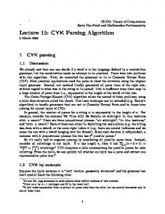
It is also possible to extend the CKY algorithm to handle some grammars which
are not in CNF. ◦ Harder to understand. Based on a “dynamic programming” ...
CKY )Cocke-Kasami-Younger) and
Earley Parsing Algorithms
Dor Altshuler
Context Free Grammar A Context-free Grammar (CFG) is a 4-tuple:
G = (N, Σ , P, S) where: N is a finite set of non-terminal symbols. Σ is a finite set of terminal symbols (tokens). P is a finite set of productions (rules). Production : (α, β) ∈ P will be written α → β where α is in N and β is in (N∪Σ)*
S is the start symbol in N.
Chomsky Normal Form A context-free grammar where the right side of each production rule is restricted to be either two non terminals or one terminal. Production can be one of following formats: ◦ A→α ◦ A → BC Any CFG can be converted to a weakly equivalent grammar in CNF
Parsing Algorithms CFGs are basis for describing (syntactic) structure of NL sentences Thus - Parsing Algorithms are core of NL analysis systems Recognition vs. Parsing:
◦ Recognition - deciding the membership in the language ◦ Parsing – Recognition+ producing a parse tree for it
Parsing is more “difficult” than recognition (time complexity) Ambiguity - an input may have exponentially many parses.
Parsing Algorithms Top-down vs. bottom-up: Top-down: (goal-driven): from the start symbol down. Bottom-up: (data-driven): from the symbols up. Naive vs. dynamic programming: Naive: enumerate everything. Backtracking: try something, discard partial solutions. Dynamic programming: save partial solutions in a table.
Examples: CKY: bottom-up dynamic programming. Earley parsing: top-down dynamic programming.
CKY )Cocke-Kasami-Younger)
One of the earliest recognition and parsing algorithms The standard version of CKY can only recognize languages defined by context-free grammars in Chomsky Normal Form (CNF). It is also possible to extend the CKY algorithm to handle some grammars which are not in CNF ◦ Harder to understand
Based on a “dynamic programming” approach: ◦ Build solutions compositionally from sub-solutions
Uses the grammar directly.
CKY Algorithm
Considers every possible consecutive subsequence of letters and sets K ∈ T[i,j] if the sequence of letters starting from i to j can be generated from the non-terminal K. Once it has considered sequences of length 1, it goes on to sequences of length 2, and so on. For subsequences of length 2 and greater, it considers every possible partition of the subsequence into two halves, and checks to see if there is some production A -> BC such that B matches the first half and C matches the second half. If so, it records A as matching the whole subsequence. Once this process is completed, the sentence is recognized by the grammar if the entire string is matched by the start symbol.
CKY Algorithm
Observation: any portion of the input string spanning i to j can be split at k, and structure can then be built using sub-solutions spanning i to k and sub-solutions spanning k to j . Meaning: Solution to problem [i, j] can constructed from solution to sub problem [i, k] and solution to sub problem [k ,j].
CKY Algorithm for Deciding CFL Consider the grammar G given by: S e | AB | XB T AB | XB X AT Aa Bb
CKY Algorithm for Deciding CFL Consider the grammar G given by: S e | AB | XB T AB | XB X AT Aa Bb 1. 2.
Is w = aaabb in L(G ) ? Is w = aaabbb in L(G ) ?
CKY Algorithm for Deciding CFL The algorithm is “bottom-up” in that we start with bottom of derivation tree. S e | AB | XB T AB | XB X AT Aa Bb
a
a
a
b
b
CKY Algorithm for Deciding CFL 1) Write variables for all length 1 substrings S e | AB | XB T AB | XB X AT Aa Bb
a
a
a
b
b
A
A
A
B
B
CKY Algorithm for Deciding CFL 2) Write variables for all length 2 substrings S e | AB | XB T AB | XB X AT Aa Bb
a
a
a
b
b
A
A
A
B
B
S,T T
CKY Algorithm for Deciding CFL 3) Write variables for all length 3 substrings S e | AB | XB T AB | XB X AT Aa Bb
a
a
a
b
b
A
A
A
B
B
S,T T X
CKY Algorithm for Deciding CFL 4) Write variables for all length 4 substrings S e | AB | XB T AB | XB X AT Aa Bb
a
a
a
b
b
A
A
A
B
B
S,T T X
S,T
CKY Algorithm for Deciding CFL 5( Write variables for all length 5 substrings. S e | AB | XB T AB | XB X AT Aa Bb
a
a
a
b
b
A
A
A
B
B
aaabb REJECTED!
S,T T X
S,T X
CKY Algorithm for Deciding CFL Now look at aaabbb : S e | AB | XB T AB | XB X AT Aa Bb
a
a
a
b
b
b
CKY Algorithm for Deciding CFL 1) Write variables for all length 1 substrings. S e | AB | XB T AB | XB X AT Aa Bb
a A
a A
a A
b B
b B
b B
CKY Algorithm for Deciding CFL 2) Write variables for all length 2 substrings. S e | AB | XB T AB | XB X AT Aa Bb
a A
a A
a b A B S,T
b B
b B
CKY Algorithm for Deciding CFL 3) Write variables for all length 3 substrings. S e | AB | XB T AB | XB X AT Aa Bb
a A
a A
a b A B S,T T X
b B
b B
CKY Algorithm for Deciding CFL 4) Write variables for all length 4 substrings. S e | AB | XB T AB | XB X AT Aa Bb
a A
a A
a b A B S,T T X S,T
b B
b B
CKY Algorithm for Deciding CFL 5) Write variables for all length 5 substrings. S e | AB | XB T AB | XB X AT Aa Bb
a A
a A
a b A B S,T T X S,T
X
b B
b B
CKY Algorithm for Deciding CFL 6) Write variables for all length 6 substrings. S e | AB | XB T AB | XB X AT Aa Bb
a A
S is included so aaabbb accepted!
a A
a b A B S,T T X
S,T
X S,T
b B
b B
The CKY Algorithm function CKY (word w, grammar P) returns table for i from 1 to LENGTH(w) do table[i-1, i] {A | A wi ∈ P } for j from 2 to LENGTH(w) do for i from j-2 down to 0 do for k i + 1 to j – 1 do table[i,j] table[i,j] ∪ {A | A BC ∈ P, B ∈ table[i,k], C ∈ table[k,j] } If the start symbol S ∈ table[0,n] then w ∈ L(G)
CKY Algorithm for Deciding CFL The table chart used by the algorithm: j i 0 1 2 3 4 5
1 a
2 a
3 a
4 b
5 b
6 b
CKY Algorithm for Deciding CFL 1. Variables for length 1 substrings. j i 0 1 2 3 4 5
1 a A
2 a
3 a
4 b
5 b
6 b
A A B B B
CKY Algorithm for Deciding CFL 2. Variables for length 2 substrings. j i 0 1 2 3 4 5
1 a A
2 a A
3 a A
4 b
S,T B
5 b
B
6 b
B
CKY Algorithm for Deciding CFL 3. Variables for length 3 substrings. j i 0 1 2 3 4 5
1 a A
2 a A
3 a A
4 b X S,T B
5 b
B
6 b
B
CKY Algorithm for Deciding CFL 4. Variables for length 4 substrings. j i 0 1 2 3 4 5
1 a A
2 a A
3 a A
4 b X S,T B
5 b S,T B
6 b
B
CKY Algorithm for Deciding CFL 5. Variables for length 5 substrings. j i 0 1 2 3 4 5
1 a A
2 a A
3 a A
4 b X S,T B
5 b X S,T B
6 b B
CKY Algorithm for Deciding CFL 6. Variables for aaabbb. ACCEPTED! j i 0 1 2 3 4 5
1 a A
2 a A
3 a A
4 b X S,T B
5 b X S,T B
6 b S,T B
Parsing results
We keep the results for every wij in a table. Note that we only need to fill in entries up to the diagonal. Every entry in the table T[i,j] can contains up to r=|N| symbols (the size of the non-terminal set). We can use lists or a Boolean n*n*r table. We then want to find T[0,n,S] = true.
CKY recognition vs. parsing Returning the full parse requires storing more in a cell than just a node label. We also require back-pointers to constituents of that node. We could also store whole trees, but less space efficient. For parsing, we must add an extra step to the algorithm: follow pointers and return the parse.
Ambiguity Efficient Representation of Ambiguities Local Ambiguity Packing : ◦ a Local Ambiguity - multiple ways to derive the same substring from a non-terminal ◦ All possible ways to derive each non-terminal are stored together ◦ When creating back-pointers, create a single back-pointer to the “packed” representation
Allows to efficiently represent a very large number of ambiguities (even exponentially many) Unpacking - producing one or more of the packed parse trees by following the back-pointers.
CKY Space and Time Complexity Time complexity: Three nested “for” loop each one of O(n) size. Lookup for r =|N| pair rules at each step. Time complexity – O(r2n3) = O(n3) Space complexity: A three dimensions table at size n*n*r A n*n table with lists up to size of r Space complexity – O(rn2) = O)n2(
or
Another Parsing Algorithm
Parsing General CFLs vs. Limited Forms Efficiency: ◦ Deterministic (LR) languages can be parsed in linear time. ◦ A number of parsing algorithms for general CFLs require O(n3) time. ◦ Asymptotically best parsing algorithm for general CFLs requires O(n2.37), but is not practical. Utility - why parse general grammars and not just CNF? ◦ Grammar intended to reflect actual structure of language. ◦ Conversion to CNF completely destroys the parse structure.
The Earley Algorithm (1970)
Doesn’t require the grammar to be in CNF. Usually moves left-to-right. Makes it faster than O(n3) for many grammars. Earley’s algorithm resembles recursive descent, but solves the left-recursion problem. No recursive function calls. Use a parse table as we did in CKY, so we can look up anything we’ve discovered so far.
The Earley Algorithm
The algorithm is a bottom-up chart parser with top-down prediction: the algorithm builds up parse trees bottom-up, but the incomplete edges (the predictions) are generated top-down, starting with the start symbol. We need a new data structure: A dotted rule stands for a partially constructed constituent, with the dot indicating how much has already been found and how much is still predicted. Dotted rules are generated from ordinary grammar rules. The algorithm maintains sets of “states”, one set for each position in the input string (starting from 0).
The Dotted Rules With dotted rules, an entry in the chart records: Which rule has been used in the analysis Which part of the rule has already been found (left of the dot). Which part is still predicted to be found and will combine into a complete parse (right of the dot). the start and end position of the material left of the dot. Example:
A X1X2…• C … Xm
Operation of the Algorithm Process all hypotheses one at a time in order. This may add new hypotheses to the end of the to-do list, or try to add old hypotheses again. Process a hypothesis according to what follows the dot:
◦ If a symbol, scan input and see if it matches. ◦ If a non-terminal, predict ways to match it. (we’ll predict blindly, but could reduce # of predictions by looking ahead k symbols in the input and only making predictions that are compatible)
◦ If nothing, then we have a complete constituent, so attach it to all its customers.
Parsing Operations The Earley algorithm has three main operations: Predictor: an incomplete entry looks for a symbol to the right of its dot. if there is no matching symbol in the chart, one is predicted by adding all matching rules with an initial dot. Scanner: an incomplete entry looks for a symbol to the right of the dot. this prediction is compared to the input, and a complete entry is added to the chart if it matches. Completer: a complete edge is combined with an incomplete entry that is looking for it to form another complete entry.
Parsing Operations
The Earley Recognition Algorithm The Main Algorithm: parsing input w=w1w2…wn 1. 2.
3. 4.
S0 = {[S → • P (0) ]} For 0 ≤ i ≤ n do: Process each item s ∈ Si in order by applying to it a single applicable operation among: (a) Predictor (adds new items to Si) (b) Completer (adds new items to Si) (c) Scanner (adds new items to Si+1) If Si+1 = Ø Reject the input. If i = n and [S→P• (0)] ∈ Sn then Accept the input.
Earley Algorithm Example Consider the following grammar for arithmetic expressions: S→P (the start rule) P→P+M P→M M→M*T M→T T → number With the input: 2 + 3 * 4
Earley Algorithm Example Sequence(0) • 2 + 3 * 4 (1)
S → • P (0)
# start rule
Earley Algorithm Example Sequence(0) • 2 + 3 * 4 S → • P (0) (2) P → • P + M (0) (3) P → • M (0) (1)
# start rule # predict from (1) # predict from (1)
Earley Algorithm Example Sequence(0) • 2 + 3 * 4 (1) (2) (3) (4) (5)
S → • P (0) P → • P + M (0) P → • M (0) M → • M * T (0) M → • T (0)
# start rule # predict from (1) # predict from (1) # predict from (3) # predict from (3)
Earley Algorithm Example Sequence(0) • 2 + 3 * 4 (1) (2) (3) (4) (5) (6)
S → • P (0) P → • P + M (0) P → • M (0) M → • M * T (0) M → • T (0) T → • number (0)
# start rule # predict from (1) # predict from (1) # predict from (3) # predict from (3) # predict from (5)
Earley Algorithm Example Sequence(1) 2 • + 3 * 4 (1)
T → number • (0)
# scan from S(0)(6)
Earley Algorithm Example Sequence(1) 2 • + 3 * 4 T → number • (0) (2) M → T • (0) (1)
# scan from S(0)(6) # complete from S(0)(5)
Earley Algorithm Example Sequence(1) 2 • + 3 * 4 T → number • (0) (2) M → T • (0) (3) M → M • * T (0) (4) P → M • (0) (1)
# scan from S(0)(6) # complete from S(0)(5) # complete from S(0)(4) # complete from S(0)(3)
Earley Algorithm Example Sequence(1) 2 • + 3 * 4 (1) (2) (3) (4) (5) (6)
T → number • (0) M → T • (0) M → M • * T (0) P → M • (0) P → P • + M (0) S → P • (0)
# scan from S(0)(6) # complete from S(0)(5) # complete from S(0)(4) # complete from S(0)(3) # complete from S(0)(2) # complete from S(0)(1)
Earley Algorithm Example Sequence(2) 2 + • 3 * 4 (1)
P → P + • M (0)
# scan from S(1)(5)
Earley Algorithm Example Sequence(2) 2 + • 3 * 4 P → P + • M (0) (2) M → • M * T (2) (3) M → • T (2) (1)
# scan from S(1)(5) # predict from (1) # predict from (1)
Earley Algorithm Example Sequence(2) 2 + • 3 * 4 P → P + • M (0) (2) M → • M * T (2) (3) M → • T (2) (4) T → • number (2) (1)
# scan from S(1)(5) # predict from (1) # predict from (1) # predict from (3)
Earley Algorithm Example Sequence(3) 2 + 3 • * 4 (1)
T → number • (2)
# scan from S(2)(4)
Earley Algorithm Example Sequence(3) 2 + 3 • * 4 T → number • (2) (2) M → T • (2) (1)
# scan from S(2)(4) # complete from S(2)(3)
Earley Algorithm Example Sequence(3) 2 + 3 • * 4 T → number • (2) (2) M → T • (2) (3) M → M • * T (2) (4) P → P + M • (0) (1)
# scan from S(2)(4) # complete from S(2)(3) # complete from S(2)(2) # complete from S(2)(1)
Earley Algorithm Example Sequence(3) 2 + 3 • * 4 (1) (2) (3) (4) (5) (6)
T → number • (2) M → T • (2) M → M • * T (2) P → P + M • (0) P → P • + M (0) S → P • (0)
# scan from S(2)(4) # complete from S(2)(3) # complete from S(2)(2) # complete from S(2)(1) # complete from S(0)(2) # complete from S(0)(1)
Earley Algorithm Example Sequence(4) 2 + 3 * • 4 (1)
M → M * • T (2)
# scan from S(3)(3)
Earley Algorithm Example Sequence(4) 2 + 3 * • 4 M → M * • T (2) (2) T → • number (4) (1)
# scan from S(3)(3) # predict from (1)
Earley Algorithm Example Sequence(5) 2 + 3 * 4 • (1)
T → number • (4)
# scan from S(4)(2)
Earley Algorithm Example Sequence(5) 2 + 3 * 4 • T → number • (4) (2) M → M * T • (2) (1)
# scan from S(4)(2) # complete from S(4)(1)
Earley Algorithm Example Sequence(5) 2 + 3 * 4 • T → number • (4) (2) M → M * T • (2) (3) M → M • * T (2) (4) P → P + M • (0) (1)
# scan from S(4)(2) # complete from S(4)(1) # complete from S(2)(2) # complete from S(2)(1)
Earley Algorithm Example Sequence(5) 2 + 3 * 4 • (1) (2) (3) (4) (5) (6)
T → number • (4) M → M * T • (2) M → M • * T (2) P → P + M • (0) P → P • + M (0) S → P • (0)
# scan from S(4)(2) # complete from S(4)(1) # complete from S(2)(2) # complete from S(2)(1) # complete from S(0)(2) # complete from S(0)(1)
The state S→P• (0) represents a completed parse.
Finding the parse tree Seq 0
Seq 1
Seq 2
Seq 3
Seq 4
Seq 5
•2+3*4
2•+3*4
2+•3*4
2+3•*4
2+3*•4
2+3*4•
T → ‘3’ • (2)
M→M*•T (2)
T → ‘4’ • (4)
T → • num (4)
M→M*T• (2)
S → • P (0)
T → ‘2’ • (0)
P→P+•M (0)
P→•P+M (0)
M → T • (0)
M → • M * T M → T • (2) (2)
P → • M (0)
M→M•*T (0)
M → • T (2)
M→M•*T (2)
M→M•*T (2)
M→•M*T (0)
P → M • (0)
T → • num (2)
P→P+M• (0)
P→P+M• (0)
M → • T (0)
P→P•+M (0)
P→P•+M (0)
P→P•+M (0)
T → • num (0)
S → P • (0)
S → P • (0)
S → P • (0)
Finding the parse tree Seq 0
Seq 1
Seq 2
Seq 3
Seq 4
Seq 5
•2+3*4
2•+3*4
2+•3*4
2+3•*4
2+3*•4
2+3*4•
S → • P (0)
T → ‘2’ • (0)
P→P+•M (0)
T → ‘3’ • (2)
M→M*•T (2)
T → ‘4’ • (4)
P→•P+M (0)
M → T • (0)
M → • M * T M → T • (2) (2)
T → • num (4)
M→M*T• (2)
P → • M (0)
M→M•*T (0)
M → • T (2)
M→M•*T (2)
M→M•*T (2)
M→•M*T (0)
P → M • (0)
T → • num (2)
P→P+M• (0)
P→P+M• (0)
M → • T (0)
P→P•+M (0)
P→P•+M (0)
P→P•+M (0)
T → • num (0)
S → P • (0)
S → P • (0)
S → P • (0)
Earley Algorithm Time Complexity
Algorithm iterates for each symbol of input (n iterations) How many items can be created and processed in Si ?
Earley Algorithm Time Complexity
Algorithm iterates for each symbol of input (n iterations) How many items can be created and processed in Si ? ◦ Each item in Si has the form [A X1X2…• C … Xm, j] ( 0 ≤ j ≤ i ) ◦ Thus O(r*n) = O(n) items.
Earley Algorithm Time Complexity
Algorithm iterates for each symbol of input (n iterations) How many items can be created and processed in Si ? ◦ Each item in Si has the form [A X1X2…• C … Xm, j] ( 0 ≤ j ≤ i ) ◦ Thus O(r*n) = O(n) items.
The Scanner and Predicator operations on an item each require a constant time.
Earley Algorithm Time Complexity
Algorithm iterates for each symbol of input (n iterations) How many items can be created and processed in Si ? ◦ Each item in Si has the form [A X1X2…• C … Xm, j] ( 0 ≤ j ≤ i ) ◦ Thus O(r*n) = O(n) items.
The Scanner and Predicator operations on an item each require a constant time. The Completer operation on an item adds items of the form [B X1X2…A•…Xm, k] to Si with 0 ≤ k ≤ i , so it may require up to O(r*n) = O(n) time for each processed item.
Earley Algorithm Time Complexity
Algorithm iterates for each symbol of input (n iterations) How many items can be created and processed in Si ? ◦ Each item in Si has the form [A X1X2…• C … Xm, j] ( 0 ≤ j ≤ i ) ◦ Thus O(r*n) = O(n) items.
The Scanner and Predicator operations on an item each require a constant time. The Completer operation on an item adds items of the form [B X1X2…A•…Xm, k] to Si with 0 ≤ k ≤ i , so it may require up to O(r*n) = O(n) time for each processed item. Time require for each iteration is thus O(r2n2) = O(n2) Time bound on the entire algorithm is therefore O(n3)
Earley Algorithm Time Complexity Earley algorithm provide better time complexity in special cases:
Earley Algorithm Time Complexity Earley algorithm provide better time complexity in special cases:
Completer is the operation that may require O(i2) time in iteration i
Earley Algorithm Time Complexity Earley algorithm provide better time complexity in special cases:
Completer is the operation that may require O(i2) time in iteration i For unambiguous grammars, Earley shows that the Completer operation will require at most O(i) time. Thus time complexity for unambiguous grammar is O(n2)
Earley Algorithm Time Complexity Earley algorithm provide better time complexity in special cases:
Completer is the operation that may require O(i2) time in iteration i For unambiguous grammars, Earley shows that the Completer operation will require at most O(i) time. Thus time complexity for unambiguous grammar is O(n2) For some grammars, the number of items in each Si is bounded by a constant (bounded-state grammars) For bounded-state grammars, the time complexity of the algorithm is linear – O(n)
CKY vs. Earley CKY is a bottom-up parser. Earley is a bottom-up parser with a top-down prediction.
CKY algorithm requires the grammar to be in CNF. Earley algorithm works for any grammar.
CKY require O(n3) time for any grammar. Earley algorithm can work in O(n2) or O(n) time for some grammars.
The End.
Thank you