Parsing nucleic acid pseudoknotted secondary structure: algorithm ...

Parsing nucleic acid pseudoknotted secondary structure: algorithm and applications Baharak Rastegari, Anne Condon The Department of Computer Science University of British Columbia Vancouver, B.C., V6T 1Z4, Canada {baharak,condon}@cs.ubc.ca August 2, 2006

Abstract Accurate prediction of pseudoknotted nucleic acid secondary structure is an important computational challenge. Prediction algorithms based on dynamic programming aim to find a structure with minimum free energy according to some thermodynamic (“sum of loop energies”) model that is implicit in the recurrences of the algorithm. However, a clear definition of what exactly are the loops in pseudoknotted structures, and their associated energies, has been lacking. In this work, we present a complete classification of loops in pseudoknotted nucleic secondary structures, and describe the Rivas and Eddy and other energy models as sum-of-loops energy models. We give a linear time algorithm for parsing a pseudoknotted secondary structure into its component loops. We give two applications of our parsing algorithm. The first is a linear time algorithm to calculate the free energy of a pseudoknotted secondary structure. This is useful for heuristic prediction algorithms, which are widely used since (pseudoknotted) RNA secondary structure prediction is NP-hard. The second application is a linear time algorithms to test the generality of the dynamic programming algorithm of Akutsu for secondary structure prediction. Together with previous work, we use this algorithm to compare the generality of state-of-the-art algorithms on real biological structures.

1

Introduction

Nucleic acids - that is, DNA and RNA molecules - play fundamental roles in the cell: in translation and replication of the genetic code, as catalysts in cellular processes, and as mediators in determining the expression level of genes [12]. Additionally, in vitro selection methods have produced nucleic acids not found in the cell, which can function as enzymes [19], or as aptamers with high binding specifity for target proteins [7, 14], with applications in medical diagnosis or as biosensors. Designed DNA and RNA molecules further expand the range of capabilities of nucleic acids. For example, rigid lattices constructed from 1

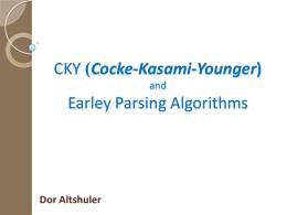
DNA can be used to organize matter with nanoscale precision [31, 32, 39]. DNA has also been used to build molecular devices that have mechanical properties [33]. Structure is key to the function of nucleic acids in their diverse roles. Thus, methods for predicting nucleic acid structure from the base sequence are of great value, in order to understand the principles of nucleic acid function, and also to aid in design of nucleic acids with novel functions. Unfortunately, 3-dimensional nucleic acid structure prediction from the base sequence of a nucleic acid is currently beyond our reach. However, there has been significant success in predicting nucleic acid secondary structure, which already can provide much useful insight as to the function of a molecule. The secondary structure is the set of base pairs that form when the molecule folds (see Figure 1 and Section 2 for details). There has been significant investment in prediction of pseudoknot free secondary structures, that is, structures with no crossing base pairs. A pseudoknot free structure is illustrated in Figure 1 (a). The figure also illustrates that the base pairs of a pseudoknot free structure naturally organize the structure into well-defined loops, and that the structure can be unambiguously represented as a string in dot-parenthesis format - a generalization of a string of balanced parentheses in which matching parentheses denote base pairs and dots denote unpaired bases. The premise underlying secondary structure prediction algorithms is that a molecule folds into that secondary structure with minimum free energy (mfe) [27], where the energy of a structure can be estimated as the sum of loop energies. Nussinov and Jacobson [26] were the first to propose a dynamic programming algorithm for mfe pseudoknot free secondary structure prediction. Since then, prediction accuracy and efficiency has improved, due to better, experimentally determined energy parameters as well as refined algorithms with O(n3 ) running time, where n is the number of bases of the molecule [21, 24]. Moreover, it is straightforward to parse a pseudoknot free secondary structure (represented in dot-parenthesis notation or any other standard notation) in linear time, in order to determine its loops and calculate its free energy. While many biological structures are pseudoknot free, pseudoknots are essential for the function of several RNA molecules in the cell [35, 37], as well as in viral RNA [11]. For example, pseudoknots form the catalytic core of some ribozymes (RNA enzymes) and selfsplicing introns (regions of messenger RNA which do not code for a protein). Pseudoknots also induce ribosomal frameshifting – a process whereby the 3-nucleotide codon reading frame is shifted, typically by ±1, thereby facilitating the synthesis of two proteins from one coding sequence [4]. Figure 1 (b) illustrates one type of pseudoknotted structure, often called a kissing hairpin, and Figure 2 includes another, called an H-type pseudoknot (concatenated with a pseudoknot free structure). In contrast with pseudoknot free structures, there is as yet no widely-agreed-upon standard model for estimating the energy of pseudoknotted structures, and little experimental data on the energy of pseudoknotted structures. Some recent theoretical work has proposed detailed energy models for simple types of pseudoknotted structures, such as H-type pseudoknots [1]. Xayaphoummine et al. [38] have also proposed a general model, in which stems (contiguous base pairs) and unpaired regions are modeled as rods and polymer chains, respectively. Pseudoknotted secondary structure prediction is NP-hard [3, 22, 23] for a simple energy model that depends on base pairs but not on unpaired bases. Lyngsø [22] shows that NP-hardness of the 2

prediction problem is sensitive to the energy model, so it is not clear whether the problem is hard for more realistic energy models. Several polynomial-time dynamic programming algorithms for pseudoknotted structure prediction have been proposed [3, 13, 28, 30, 36]. Underlying each of these algorithms is a sum-of-loops energy model for pseudoknotted structures: given a sequence, each algorithm reports the structure with the minimum free energy for that sequence, from a restricted class of structures, according to a fixed energy model. We say that a structure R can be handled by an algorithm if R is in the class of structures over which the algorithm optimizes (according to the algorithm’s energy model). Algorithms for pseudoknotted secondary structure prediction differ in their run-time complexity and their generality, that is, the class of structures that they handle. For example, kissing hairpin structures are not in the class of structures handled by the algorithms of Akutsu [3] and Dirks and Pierce [13], but are in the class handled by Rivas and Eddy’s algorithm [30]. (We emphasize that, even when the true structure R for a sequence is handled by an algorithm, this does not necessarily mean that the algorithm correctly predicts R, because correctness depends not only on the generality of the algorithm but also on the energy model and parameters being used for the free energy calculation.) The O(n6 ) algorithm of Rivas and Eddy [30] handles (that is, predicts a structure from) the most general class of structures. However, the loop types and thermodynamic model underlying the Rivas and Eddy algorithm are specified only implicitly in the recurrence equations of the algorithms. There is not a one-to-one correspondence between loops and terms in the recurrence equations, making it difficult to infer the loop types directly from the recurrences. Prior to our work, there has been no algorithm that, given a sequence and a pseudoknotted secondary structure for that sequence, calculates its free energy. In this work we present the first comprehensive classification of loops that arise in pseudoknotted secondary structures. Previous classifications apply to a restricted range of structures [18], and do not address the problems of defining and calculating the energy of a structure. Our classification is inspired by the algorithm of Rivas and Eddy, and we use it to describe the energy model of Rivas and Eddy and other algorithms as a sum-ofloops model. Building on an algorithm of Bader et al. [5], we show how to parse a given secondary structure into its component loops in linear time. We present two applications of this parsing algorithm. First, we show how to calculate the free energy of a pseudoknotted secondary structure in linear time. This can be useful in heuristic algorithms, which are commonly used for pseudoknotted secondary structure prediction [2, 17, 29], and which typically repeatedly estimate the energy of a candidate structure. The second application of our parsing algorithm is an assessment of the trade-off between generality and efficiency of dynamic programming algorithms for RNA secondary structure prediction. As noted above, each dynamic programming algorithm only predicts structures from a restricted class. Let A, D&P, L&P and R&E denote the classes of structures handled by the Akutsu [3], Dirks and Pierce [13], Lyngsø and Pedersen, [23], and Rivas and Eddy [30] algorithms, respectively. For example, the algorithm of Rivas and Eddy

3

handles kissing hairpin structures, but the other algorithms do not. In previous work [9], we obtained linear time tests for membership in the L&P, D&P and R&E classes. In this paper, we apply the parsing algorithm to give a linear time test for membership in Akutsu’s class. We provide a comparison of all four algorithms on a set of several hundred biological structures. The results show that the Dirks and Pierce class handles more or less the same structures as does Akutsu’s class, so the extra level of generality provided by Akutsu’s class is not significant, with respect to the structures found in biological organisms. We also add to our comparison another class, called the density 2 structures. This class is interesting because there is an O(n3 ) algorithm to predict stuctures in this class, based on the principle of hierarchical folding [40]. We find that the density 2 structure class contains many more biological structures than does Akutsu’s class, while still being a little less general than the Rivas and Eddy class on our dataset. The rest of paper is organized as follows. In Section 2, we define the components of a pseudoknotted secondary structure. In Section 3 we present our linear-time parsing algorithm. In Section 3.2 we present our algorithm for enumerating the loops of a secondary structure, and describe how to calculate the free energy of a secondary structure in Section 4. Our algorithm for testing membership in Akutsu’s class is in Section 5, followed by conclusions in Section 6.

2

Components of a Pseudoknotted Secondary Structure

We model an RNA molecule as a string, with distinct ends, called the 5′ (left) and 3′ (right) ends, over a finite alphabet. (The alphabet symbols include A, C, G, and U which denote the bases Adenine, Guanine, Cytosine, and Uracil, respectively, but may include other symbols, such as those of the IUPAC code which express ambiguity at certain positions [10].) Throughout, we use n to denote the length of the sequence. We index the bases consecutively from 1 to n, starting from the 5′ end, and refer to a base by its index. An RNA molecule folds into a functional structure by formation of bonds between pairs of bases, where each base may pair with at most one other base. We use i.j to denote the base pair involving bases i and j. A secondary structure is a set of base pairs. Figure 1 (a) and (b) give graphical depictions of RNA secondary structures. We let bp(i) denote the base that is paired with base i, if any; otherwise if i is unpaired, bp(i) = 0. Two base pairs i.j and i′ .j ′ cross if i < i′ < j < j ′ . We say that pair i.j is pseudoknotted if it crosses some base pair. In Section 2.3 we classify loops in a pseudoknotted structure, working from the Rivas and Eddy algorithm [30]. We first introduce some other useful concepts, namely closed regions and bands. In the rest of this section, definitions are with respect to a fixed secondary structure R over a sequence with n bases.

4

2.1

Closed Regions

When 1 ≤ i ≤ j ≤ n, we use [i, j] to denote the set of bases {i, i + 1, . . . , j}, which we call a region. We call i and j the left and right borders of the region [i, j]. We say that a region is empty if no bases in the region are paired. Region [i′ , j ′ ] is nested in [i, j] if i < i′ < j ′ < j and the two regions are disjoint if j < i′ or j ′ < i. A region is weakly closed if no base pair connects a base in the region to a base outside the region. A weakly closed region [i, j] with i < j is closed if [i, j] cannot be partitioned into two smaller weakly closed regions. For example, for the structure of Figure 1 (a), [5,68] is closed region. [6,66] is weakly closed but not closed, since it can be decomposed into two weakly closed regions [6,6] and [7,66], and [10,65] is weakly closed but not closed, since it can be decomposed into two weakly closed regions [10,25] and [26,65]. Let 1 ≤ i, j ≤ n. Formally, [i, j] is weakly closed iff for all base pairs i′ .bp(i′ ) of R, i′ ∈ [i, j] if and only if bp(i′ ) ∈ [i, j]. Also, [i, j] is closed iff i < j, [i, j] is weakly closed, and for all l ∈ [i, j − 1], neither [i, l] nor [l + 1, j] is weakly closed. Note that if [i, j] is closed then both i and j must be paired (although not necessarily with each other): if i were unpaired, for example, then both [i, i] and [i + 1, j] would be weakly closed. To simplify later definitions, we also declare [0, n + 1] to be closed. In what follows, whenever we refer to closed region [i, j], we mean a closed region with 1 ≤ i < j ≤ n. We will always handle the special case [0, n + 1] explicitly. Let [i, j] be a closed region. If bp(i) = j then we say that the region has one closing base pair, namely i.j. Otherwise, we say that i.bp(i) and bp(j).j are the closing base pairs of the region; in this case, we say that the closed region is pseudoknotted. The closed region [0, n + 1] has no closing base pair. Let [i, j] and [i′ , j ′ ] be closed regions. We say that [i′ , j ′ ] is a child of [i, j] if [i′ , j ′ ] is nested in [i, j] and is not nested in any closed region [i′′ , j ′′ ] with i < i′′ . If [i′ , j ′ ] is not a child of any closed region [i, j] with 1 ≤ i < j ≤ n, then we say that [i′ , j ′ ] is a child of [0, n + 1]. Closed regions of a structure are organized hierarchically, as illustrated in Figure 2. That is, two closed regions [i, j] and [i′ , j ′ ] with i < i′ are either nested or disjoint. The closed regions tree of R is denoted by T (R), with the nodes of T (R) being the closed regions of R. The root is [0, n + 1]. The children of node [i, j] or [0, n + 1] are the closed region children of region [i, j] or [0, n + 1], respectively. The children of each node are ordered (from left to right) by their left border. We conclude this section with some simple facts about closed regions that will be useful in a later proof. Claim 2.1 Let R be a structure on n bases. (a) Every base pair of R is in some closed region child of [0, n + 1]. (b) The rightmost paired base of R is the rightmost border of a closed region that is a child of [0, n + 1]. 5

(a) C G P A T U G *C U G *C C *G C *G D C U* C 66

G 68 G 73 C A U G U G G* C C A G* C* C C U G * *C A U G* G* A U G R K * O P G * *C A G C*G C 5 *C 7 C G*C 25 1 G 10 U G*G I U G*U A A D G G D G C

76

(((((.(..( (((....... .)))).(((( (.......)) ))).....(( (((....... )))))).))) )).... (b) 55

43

A C C C U A C U G U G C U 70 62 *G G* G* A* U* G* A* C* * * * * A U G G C A A U A G A C C A A G C C A A G A A G U A A A U U C C U U * U* C* G* G* U* U U U A G A U U G A U C C G C A U * 82 * A* G* * A* A A* G* G* C* * U * A* C* U* U* U* A* A* C* G A A U G A A A 88

40

30

20

95

90 10

110

U

108

97

103

A G A U*A U*A U*A U*A

1

114

Figure 1: (a) Graphical depiction of the secondary structure of a transfer RNA molecule from the Sprinzl database (RA7630) [34], and dot-parenthesis representation of the structure. A grey line links bases in order, and a black mark between two bases indicates a base pair. (b) Graphical depiction of a pseudoknotted structure found in the coxsackie B virus. This structure, called a kissing hairpin [25] or a HH-type pseudoknot [18], is essential for replication of the virus [11, 25]. Figures generated using the Pseudoviewer web service [18].

6

10

A C U

25

A C

15

U C C G*

5

C

U

U

U

29 U C *A C C * G A C *G G A * C C * C * G G *G *U C C G* C *G 40 A G* A 36 C U 17

U A*

C

1

(a)

18

44

32

[0,45] [18,40]

[1,17] [2,16] [3,15] [4,14] [5,13]

(b)

Figure 2: Hierarchical representation of a secondary structure. (a) Secondary structure fragment of turnip yellow mosaic virus (TYMV) [20] (generated using Pseudoviewer [18]. (b) Tree showing hierarchical organization of closed regions of the TYMV structure fragment. Proof (a) The smallest closed region containing a base pair must be a subset of [1, n]. This region is either a child of [0, n + 1] or a descendent of [0, n + 1]. In either case, the base pair is in a child of [0, n + 1]. (b) If j is the rightmost paired base, and is paired with i (< j), then i.j is in some closed region C in [1, n]. It must be that j is the rightmost border of C since there is no base greater than j which could be the right border of C. C must be a child of [0, n + 1] since it cannot be nested in any other closed region in [1, n], again since no base to the right of j is paired.

2.2

Bands

Loosely speaking, a band is a “pseudoknotted stem”. For example, in Figure 1 (b), the union of the paired regions [43,54] and [71,82] is a band. This structure has three bands in total, the other two being [56,61] ∪ [97,102] and [88,95] ∪ [103,110]. Formally, let i.j and i′ .j ′ be pseudoknotted base pairs. We say that i′ .j ′ is directly banded in i.j and write i′ .j ′  i.j if

7

1. i < i′ < j ′ < j, 2. for all a.b ∈ R, a.b crosses i.j if and only if a.b crosses i′ .j ′ , and 3. the regions [i + 1, i′ − 1] and [j ′ + 1, j − 1] are weakly closed. Let i′ .j ′ = i1 .j1  i2 .j2  . . . ik .jk = i.j be a maximal chain of base pairs with respect to the  relation. (Note that k may equal 1, in which case i′ = i and j ′ = j.) We call [i, i′ ] ∪ [j ′ , j] a band. For each l, 1 ≤ l ≤ k − 1, we call [il , il+1 ] ∪ [jl+1 , jl ] a band segment. Base pairs i′ .j ′ , i.j are the band’s inner and outer closing pairs, respectively, and i and j are the left and the right borders of the band, respectively. The base pairs il .jl , 1 ≤ l ≤ k span the band.

2.3

Loops

For pseudoknot free structures, loops are most naturally seen in traditional graphical diagrams - see Figure 1 (a). Every unpaired base is in one loop, and every base pair is in exactly two loops. Here, we extend definitions of loop to pseudoknotted structures. Our primary motivation is to provide a framework for describing the energy models used by dynamic programming algorithms for pseudoknotted secondary structure prediction. Our definitions have the property that every unpaired base is in exactly one loop and every base pair is in at most three loops. Our definitions of hairpin and interior loops are the same as for pseudoknot free structures; we include them here for completeness. We then provide definitions of multiloops and external loops, including cases in which pseudoknotted closed regions are nested in such loops. Finally, we define a new type of loop, namely a pseudoloop, which includes the unpaired bases of a pseudoknotted closed region, as well as the base pairs that are adjacent to these unpaired bases. We expect that our definition of pseudoloop will need to be refined in the future, to further distinguish between the energy contributions of different pseudoloop subtypes, as more understanding of pseudoknotted energies is gained. Currently, however, dynamic programming algorithms use a single rule for estimating the energy of all pseudoloops that are within the range of structures that the algorithms can handle. We use the following notation. We say that band [i, i′ ] ∪ [j ′ , j] is associated with closed region [i′′ , j ′′ ] if [i, i′ ], and thus [j ′ , j], are nested in [i′′ , j ′′ ] but not in any (closed region) child of [i′′ , j ′′ ]. For example, in Figure 1 (b), the three bands [43,54] ∪ [71,82], [56,61] ∪ [97,102] and [88,95] ∪ [103,110] are associated with closed region [43,110]. No bands are ever associated with [0, n + 1]. The unpaired bases associated with closed region [i, j] are the unpaired bases in [i, j] but not in any closed region or band segment which is nested in [i, j]. For example, in the structure of Figure 1 (b), the unpaired bases associated with closed region [43,110] are 55, 62-70, 83-87, and 96. If i′ .j ′  i.j, then the unpaired bases associated with band segment [i + 1, i′ − 1] ∪ [j ′ + 1, j − 1] are the unpaired bases which are in regions [i + 1, i′ − 1] or 8

[j ′ + 1, j − 1] but which are not in any closed region nested in these regions. For example, unpaired bases 90 and 108 are associated with [89,91] ∪ [107,109]. Finally, the unpaired bases associated with [0, n + 1] are the unpaired bases that are not associated with any other closed region or band segment. For example, in the structure of Figure 1 (a), the unpaired bases associated with closed region [0, 77] are 73-76. The following claim follows easily from these definitions. Claim 2.2 Any unpaired base is associated with exactly one band segment or closed region (but not both). The base pairs associated with closed region [i, j] are the closing base pairs of the region, as well as the closing base pairs of any closed region children of [i, j] which are not in any band associated with [i, j]. Similarly, the base pairs associated with closed region [0, n + 1] are the closing base pairs of any closed region children of [0, n + 1]. Let i′ .j ′  i.j, let B be the band spanned by i′ .j ′ and i.j (note that B may possibly also be spanned by other base pairs), and let B be associated with closed region [i′′ , j ′′ ]. Then the base pairs associated with band segment [i, i′ ] ∪ [j ′ , j] are the base pairs i.j, i′ .j ′ , together with the closing base pairs of closed region children of [i′′ , j ′′ ] which are in [i+, i′ − 1] or [j ′ + 1, j − 1]. Note that a base pair may not be associated with any closed region, specifically if it is not the closing base pair of a region. In this case, the base pair spans a band. Also, a base pair that is associated with one closed region must also be associated with a band segment, and a base pair that is associated with two closed regions is not associated with a band segment. The next claim summarizes these facts. Claim 2.3 Any base pair is associated with zero, one, or two closed regions. A base pair which is not associated with any closed region must span a band. A base pair which is associated with one closed region is also associated with a band segment. We are now ready to define loops. Each loop is a collection of base pairs and unpaired bases, called the members of the loop. Hairpin loop: Let i.j be a base pair such that all bases in [i + 1, j − 1] are unpaired. Then i.j is the base pair of a hairpin loop, and the bases in [i + 1, j − 1] are the unpaired bases of the loop. Interior loop: Let i.j, i′ .j ′ be base pairs with i < i′ < j ′ < i, such that regions [i+1, i′ −1] and [j ′ + 1, j − 1] are empty. Then i.j, i′ .j ′ are base pairs of an internal loop, and the bases in [i + 1, i′ − 1] and [j ′ + 1, j − 1] are the unpaired bases of the loop. An internal loop is called a stacked pair if i′ = i + 1 and j ′ = j − 1, and is called a bulge loop if either i′ = i + 1 or j ′ = j − 1, but not both. The pair i.j is the closing base pair of the loop. Note that there are two types of interior loops: those for which i.j is not pseudoknotted (in which case i′ .j ′ is also not pseudoknotted) and those for which i.j is pseudoknotted (in which case i′ .j ′ is also pseudoknotted) . In the latter case, i′ .j ′  i.j and we say that the interior loop spans a band. 9

External loop: The external loop consists of all unpaired bases and base pairs associated with closed region [0, n + 1]. Multiloop: As with interior loops, multiloops are of two types, depending on whether or not they span a band. To define the first type, let [i, j] be a closed region which is not pseudoknotted (that is, i.j ∈ R) and which either has at least two (closed region) children, or one pseudoknotted child. Then the unpaired bases and base pairs associated with [i, j] form a multiloop. For the second type of multiloop, let i.j be a pseudoknotted base pair and let i′ .j ′  i.j, where at least one of the (weakly closed) regions [i+1, i′ −1] and [j ′ +1, j −1] is not empty. Then the unpaired bases and base pairs associated with band region [i, i′ ] ∪ [j ′ , j] comprise a multiloop. We say that the multiloop spans a band. For both types of multiloop, we say that i.j is the closing base pair of the multiloop. Pseudoloop: Let [i, j] be a pseudoknotted closed region. Then the unpaired bases and base pairs associated with [i, j], together with the closing base pairs of the bands associated with [i, j], are members of a pseudoloop. The base pairs i.bp(i) and bp(j).j are the closing base pairs of the pseudoloop. Claim 2.4 There is a 1-1 correspondence between the set of all closed regions and the set of loops that do not span bands. Proof The 1-1 correspondence is as follows. The external loop and the closed region [0, n + 1] correspond to each other. Let [i, j] be a closed region, 1 ≤ i, j ≤ n. If [i, j] is not pseudoknotted, then i.j closes either a hairpin, interior, or multiloop which does not span a band, and i.j closes no other loop. The region [i, j] and the loop closed by i.j are in 1-1 correspondance with each other. If [i.j] is pseudoknotted, then i.bp(i) and bp(j).j close a pseudoloop, and close no other loop that does not span a band. Thus there is a 1-1 correspondence between pseudoknotted closed regions [i, j] and pseudoloops closed by i.bp(i) and bp(j).j. Claim 2.5 Each unpaired base is a member of exactly one loop and each base pair is a member of at least one and at most three loops. Proof First, consider the unpaired bases. By Claim 2.2, each unpaired base is associated with at most one closed region or band. Unpaired bases associated with closed region [i, j] are members of the loop that corresponds to closed region [i, j] (see Claim 2.4), and members no other loop. Finally, the unpaired bases which are associated with a band segment are members of either an interior loop or multiloop that spans the band, and are members of no other loop. Next, consider the base pairs. By Claim 2.3, each base pair is associated with zero, one, or two closed regions. First, suppose that i.j is associated with two closed regions. Then it is a member of the two loops that correspond to these closed regions. Additionally, if 10

i.j spans a band and is not the only base pair spanning the band, then i.j is a member of a single loop that spans the band, since i.j must be an outer closing base pair of the band. Thus, i.j is a member of either two or three loops. Next, suppose that i.j is associated with one closed region. Then it is a member of the loop that corresponds to this closed region. By Claim 2.3, i.j must also be associated with a band segment, in which case it is a member of a multiloop that spans a band. Additionally, if i.j itself spans a band, then as for the previous case, it is a member of at most one loop that spans the band. Overall, i.j is a member of at most three loops. Finally, suppose that i.j is associated with no closed region. Then i.j surely spans a band. If i.j is a closing base pair of the band, then it is a member of a pseudoloop. If additionally i.j is not the only base pair spanning the band, then i.j is a member of one loop that spans the band. Otherwise, i.j is not the closing base pair of a band, in which case it is a member of at most two loops that span the band. In either case, i.j is a member of at most two loops. Claim 2.5 implies that any structure for a strand of length n has O(n) loops.

3

Parsing Algorithm

A structure can be parsed into its component loops in two steps. In the first (Section 3.1), the tree of closed regions is built. In the second (Section 3.2), the tree is traversed and the list of base pairs in each loop is output.

3.1

Building the tree of closed regions

The Build-Closed-Regions-Tree Algorithm (Algorithm 1) takes as input a description of the base pairs of a secondary structure R, and outputs the closed regions tree for the structure. The algorithm runs in linear time. The algorithm is adapted slightly from an algorithm of Bader et al. [5], which constructs a forest of connected components in an overlap graph. Bader et al. applied this algorithm to the problem of computing the inversion distance between signed permutations. Scanning the structure from left to right, and using a stack, the algorithm keeps track of regions that might be closed. We call such regions potentially closed and give a formal definition in the proof of Claim 3.1. When a new base is scanned, there are three possibilities: a new potentially closed region is identified, and added to the stack (line 4); two or more potentially closed regions are merged, when a base pair linking them is identified (lines 6-8); or a potentially closed region is confirmed to indeed be closed, in which case the region is added to the tree of closed regions (line 10). For a pseudoknot free structure, potentially closed regions are never merged, and so nothing happens in lines 6-8.

11

algorithm Build-Closed-Regions-Tree input: the base pair function bp for a secondary structure R (for example, as an array bp[1, . . . , n]) output: tree T of closed regions of R 1 2 3 4

5 6 7 8 9

initialize T to contain one (unlabeled) node; initialize the stack to be empty; for λ := 1 to n { if (λ < bp(λ)) {Push([λ, bp(λ)])} // note: lines 5-9 do nothing when bp(λ).λ is not pseudoknotted elseif (0 < bp(λ) < λ) { E := λ; while (Top.B > bp(λ)) {E := max(E, Pop.E)} Top.E := max(E, Top.E) }

10 if (λ = Top.E) {Add-To-Tree(Pop)} 11 } 12 return T

procedure Add-To-Tree([i, j]) // Adds closed region [i, j] to tree T ; assumes regions are added in postfix order // and that initially the tree consists of a single node, [0, n + 1]. 1 2 3 4 5 6 7

create a new node and label it [i, j]; let [a, b] be the child of [0, n + 1] with largest left border, or [0, 0] if T has no children while (a > i) { make [a, b] a child of [i, j]; update [a, b] to be the child of T with largest left border, or [0, 0] if there are no more children } make [i, j] a child of [0, n + 1]

Algorithm 1: Building the tree of closed regions. In the algorithm, we use the notation [Top.B, Top.E] to denote the contents of the top of the stack, which is always a region.

12

Claim 3.1 The Build-Closed-Regions-Tree Algorithm adds closed regions to the tree in postfix order and runs in linear time. Proof To prove the claim, we explain how potentially closed regions are tracked by the algorithm, as the structure is scanned from left to right. We need to first define what is a potentially closed region. Intuitively, at the λth iteration of the algorithm on input structure R, a potentially closed region from the viewpoint of λ is a region that might possibly be closed (with respect to structure R), based on information gathered while scanning bases up to λ, but it is not possible yet to be sure that the region is closed. For example, in the structure of Figure 2, [1, 17] and [2, 16] are potentially closed from the view point of 10. Informally, this is because when base 1 was scanned, since base 1 is paired with base 17, it’s plausible that [1, 17] is a closed region. Similarly, when base 2 is scanned, it’s plausible that [2, 16] is a closed region. As bases 3 through 10 are scanned, we find no evidence to contradict the possibility that [1, 17] and [2, 16] are closed. Moreover, we still can’t be sure that [1, 17] and [2, 16] are closed, because at the time we scan base 10 we know nothing about the base pairs involving bases 11 through 15, and if one of these were paired with, say, base 18, then neither [1, 17] nor [2, 16] would be closed. However, region [2, 16] is not potentially closed with respect to 16, since when base 16 is scanned, we can be sure that [2, 16] is closed. However, we consider [1, 17] to be potentially closed from the viewpoint of 16. (One could argue that in fact we can conclude that [1, 17] is definitely closed once we scan base 16, since we also know that 1 is paired with 17 and there are no bases between 16 and 17 that could cause [1, 17] not to be closed. However, the algorithm does not make such inferences, and our formal definition of potentially closed regions accounts for this.) Definition 3.1 (Potentially closed regions) Let R be a secondary structure. Let R(λ) be the set of base pairs i.j of R with j ≤ λ. For any i such that 1 ≤ i ≤ λ and i < bp(i), let R(λ, i) = R(λ) ∪ {i.bp(i)}. (a) We say that i is potentially the left border of a closed region, from the viewpoint of λ iff i satisfies the following properties: (i) i is the left border of a closed region, which we denote by Cλ,i , with respect to structure R(λ, i), and (ii) Cλ,i is a child of [0, n + 1] (with respect to R(λ, i)). (b) We say that [i, j] is potentially closed from the viewpoint of λ iff (i) i ≤ λ < j, (ii) i is potentially the left border of a closed region, Cλ,i , from the viewpoint of λ, and 13

(iii) either λ < bp(i) = j or bp(i) ≤ λ and j is the largest base such that bp(j) is in Cλ,i . As another example, [18, 32], [19, 31] and [20, 30] are all of the potentially closed regions from the viewpoint of 24. These three regions, plus [25, 40], [26, 39], [27, 38], [28, 37], and [29, 36] are all of the potentially closed regions from the viewpoint of 29. From the viewpoint of 30, however, the potentially closed regions are [18, 32], [19, 31] and [20, 40]. We first show that the algorithm maintains the following invariant. Every time that line 9 of the algorithm is reached, the stack contains all potentially closed regions from the viewpoint of λ plus the closed region with λ as right border, if any, in increasing order of left border from bottom to top of the stack. Furthermore the stack contains nothing else. This is straightforward to prove by induction on λ. We give the argument for proving the induction step. Note first that if the induction hypothesis holds at line 9 for λ − 1, then if there is a closed region with right border λ − 1, it is removed in line 10. Now, consider when line 9 is reached on λ. There are three cases. The first case is when λ is unpaired. In this case, R(λ−1) = R(λ), and so the regions which are potentially closed from the viewpoint of λ − 1 are exactly those which are potentially closed from the viewpoint of λ. Also, the stack does not change in this case when lines 4-8 are executed on λ, so by induction, the stack must contain all of the potentially closed regions from the viewpoint of λ. The second case is when λ < bp(λ). In this case, [λ, bp(λ)] is a potentially closed region from the viewpoint of λ but not λ − 1, and is added to the stack in line 4 on the λth iteration of the for loop. Moreover, all other regions on the stack, which by induction are potentially closed from the viewpoint of λ − 1, are also potentially closed from the viewpoint of λ, again since R(λ − 1) = R(λ). The third case is when 0 < bp(λ) < λ. In this case, R(λ − 1) ∪ {bp(λ).λ} = R(λ). The base pair bp(λ).λ witnesses the fact that all regions [i, j] on the stack with bp(λ) < i are not potentially closed from the viewpoint of λ. This is because i cannot be a potential left border of a closed region from the viewpoint of λ. To see this, suppose that i satisfies property (i) of Definition 3.1 (a), that is, i is the left border of closed region Cλ,i , with respect to structure R(λ, i). Since bp(λ) < i, Cλ,i must be nested in [bp(λ), λ] – otherwise the base pair bp(λ).λ would connect a base, namely bp(λ), outside region Cλ,i with a base, namely λ, inside Cλ,i ), contradicting the fact that Cλ,i is closed with respect to R(λ, i). Since Cλ,i is nested in [bp(λ), λ], it cannot be the case that Cλ,i is a child of [0, n + 1], and so i fails to satisfy property (ii) of Definition 3.1 (a). Therefore, i is not a potential left border of a closed region from the viewpoint of λ. Regions [i, j] on the stack with bp(λ) < i are removed from the stack in line 7. Suppose that [i′ , j ′ ] is at the top of the stack at the end of line 7. We claim that i′ is potentially the left border of a closed region, namely the region Cλ−1,i′ ∪[bp(λ), λ], from the viewpoint of λ. This claim follows immediately from the following three facts, which we show next: (i) Cλ−1,i′ ∪ [bp(λ), λ] is a region, (ii) region Cλ−1,i′ ∪ [bp(λ), λ] is in fact closed, 14

and (iii) region Cλ−1,i′ ∪ [bp(λ), λ] is a child of [0, n + 1] (with respect to R(λ). Fact (i) follows if we show that bp(λ) ∈ Cλ−1,i′ . If i′ = bp(λ), then (i) is trivially true. So, suppose that i′ < bp(λ). Then, [bp(λ), λ] is not a potentially closed region with respect to R(λ − 1) – otherwise, [bp(λ), λ] would be above [i′ , j ′ ] on the stack. It must then be the case that [bp(λ), λ] does not satisfy property (i) of Definition 3.1 (a) of the definition of potentially closed region (Definition 3.1). (If [bp(λ), λ) satisfied part (i) (a), then it would satisfy the rest of the definition. In particular, the fact that λ is the rightmost paired base of R(λ) would imply that [bp(λ), λ] is a child of [0, n + 1] with respect to R(λ − 1, bp(λ)) = R(λ), by Claim 2.1 (b). But if [bp(λ), λ] fails to satisfy part (i) (a) with respect to λ − 1, then some base pair B in R(λ − 1) must cross bp(λ).λ. Let C be the child of [0, n + 1], with respect to R(λ − 1), containing base pair B (C must exist, by Claim 2.1 (a)). Let i′′ be the left endpoint of C. Then, bp(i′′ ) is also in C (since C is closed), and so bp(i′′ ) ≤ λ − 1. Therefore, C is a closed region with respect to R(λ−1, i′′ )(= R(λ−1)), and so i′′ is the left border of a closed region with respect to R(λ − 1). Furthermore, C must be the rightmost child of [0, n + 1] (with respect to R(λ − 1)) whose left endpoint is at most bp(λ), since it includes bp(λ). Moreover, the maximum base j ′′ > λ − 1 with bp(j ′′ ) in C exists, since in particular λ is such that bp(λ) is in C. Therefore, the top of the stack at the end of line 7 must be [i′′ , j ′′ ], and so i′ = i′′ . Therefore, C = Cλ−1,i , and thus Cλ,i contains bp(λ). Fact (ii), that region Cλ−1,i′ ∪ [bp(λ), λ] is closed with respect to R(λ), follows since Cλ−1,i′ is closed and there can be no base pair between a base less than i′ and a base in the range [bp(λ), λ]. If such a base pair existed, then it would be contained in some closed region, say C ′ , in [1, n] (by Claim 2.1 (a)). Then, Cλ−1,i′ would necessarily be a descendent of C, so Cλ−1,i′ would not be a child of [0, n + 1]. Fact (iii), that closed region Cλ−1,i′ ∪ [bp(λ), λ] must be a child of [0, n + 1] with respect to R(λ) follows from Claim 2.1 since the right border of the region is λ and λ is the rightmost paired base of R(λ. In line 8, j ′ is replaced by jmax , where jmax is the maximum of j ′ and the rightmost borders of all of the removed regions. Thus, by construction, jmax is the largest base such that bp(jmax ) is in Cλ,i′ = [i′ λ]. So, [i, jmax ] is indeed potentially closed with respect to λ or, if jmax = λ, is indeed closed. Finally, all other regions below [i′ , jmax ] on the stack are still potentially closed with respect to λ. To see this, let [i′′ , j ′′ ] be such a region. The right border of Cλ−1,i′′ must be less than bp(λ), since [i′′ , j ′′ ] is not at the top of the stack in line 7. Furthermore, j ′′ must be greater than λ − 1, and thus must be greater than λ, since bp(j ′′ ) is in Cλ−1,i′′ . From this, it follows that [i′′ , j ′′ ] must satisfy all of the conditions of a potentially closed region from the viewpoint of λ. This completes the proof of the invariant. It follows from the invariant that at line 10, if there is a closed region with right border λ, it is added to the tree on the λth iteration of the for loop. Finally, closed regions are added to the tree in postfix order because regions are added in the order of their right border. The total number of steps per iteration of the for loop, excluding the while loop of step 7, is constant. Over all runs of for loop, the while loop is called at most n times. The number of assignment statements over all executions of while loop is also bounded by at

15

most n, since stack is popped at each assignment statement, and at most n tuples are pushed onto the stack. Finally, the Add-To-Tree procedure takes O(n) time over all calls, since the time taken to add a node to the tree is proportional to the number of its children. The linear running time follows.

3.2

Enumerating Loops

Each loop is fully specified by its member base pairs: that is, the unpaired bases that are members of the loop can be inferred from the base pairs. Thus it is sufficient for an enumeration algorithm to list the base pairs of each loop, for example, with the closing base pairs first and the remaining base pairs in ordered by left index. From Claim 2.4, there is a 1-1 correspondence between closed regions and loops which do not span a band. A traversal of the closed regions tree in prefix order suffices to enumerate such loops: when visiting closed region [i, j], its closing base pairs and those of its children (in order) are the needed base pairs. To enumerate loops that span the bands associated with closed region [i, j], the following steps are needed. 1. Create an ordered list, BL(i, j), of the bases k for which either k.bp(k) or bp(k).k spans a band associated with region [i, j]. Let Succ(k) and Pred(k) denote k’s successor and predecessor in the list, respectively (with Nil indicating that k has no successor or predecessor). 2. Let nested(k) be the list of closed region children of [i, j] that are nested in region [k, Succ(k)]. 3. Scanning BL(i, j) from left to right, for each base k in BL(i, j), if k < bp(k) and Succ(k) = bp(Pred(bp(k))), then k.bp(k) is the closing base pair of a loop that spans a band. The loop is an interior loop if both nested(k) and nested(Pred(bp(k))) are Nil. Otherwise, the loop is a multiloop, and the base pairs which are members of the loop are the closing base pairs of the regions in nested(k) and nested(Pred(bp(k))), as well as the base pair Succ(k).Pred(bp(k)). All of the lists BL(i, j) can be constructed in linear time, by starting with a linked list L of all paired bases between 1 to n in order, with pointers from an array to list elements to allow direct access to any element of the list. From L, the lists BL(i, j) can be constructed by traversing the closed regions tree in postfix order, removing from list L the part that is associated with each closed region. Once the lists BL(i, j) are constructed, it is straightforward to then construct the nested(i) lists. Thus, the total running time is again linear.

16

4

Energy Model and Calculation

In the standard thermodynamic model for pseudoknot free secondary structures, the energy of a loop is a function of (i) loop type, (ii) an ordered list of its member base pairs, (iii) the bases forming each member base pair, and (iv) the unpaired bases which are members of the loop and are adjacent to each member base pair (if any). The energy of a secondary structure is then calculated by summing the free energy of its component loops. For pseudoknotted structures, the standard thermodynamic model is extended so that the energy of a loop depends additionally on (v) the location status of the loop, which indicates its position relative to pseudoloops in the structure. The location status can be one of the following. span-band : Interior or multiloops that span a band are called span-band loops. in-band : A loop that corresponds to closed region [i, j] is an in-band loop if i.j is associated with a band segment. out-band : A loop that corresponds to closed region [i, j] is an out-band loop if it is a child of a pseudoknotted closed region and is not an in-band loop. standard : Loops that are not of the three types above are called standard loops. Such loops do not span bands and are do not correspond to children of pseudoknotted loops.

4.1

Energy Calculation

It is straightforward to extend the loop enumeration algorithm so that the loop’s type and location status is output in addition to its list of tuples. For example, the type of a loop corresponding to a closed region can be determined from the number and types of its children (e.g. if the closed region is not pseudoknotted and has no children, it must be a hairpin loop; if it has one child which is not a pseudoknotted closed region then it must be an internal loop). The location status of a loop can be determined using additionally the ordered list of band segments of its parent (if any). Then the free energy of the structure can be calculated by adding up the free energy of all loops.

4.2

Discussion

In the Rivas and Eddy model [30], the energy of a loop is exactly as in the standard model for pseudoknot free structures if the loop does not span a band. The standard model is generalized in the case of multiloops, which may now contain pseudoknotted regions, as follows: the energy is of the form a + bu + ch + dm, where a, b, c, and d are constants independent of the loop, u is the number of unpaired bases of the loop, h is the number of tuples (i, j) of the multiloop with i · j ∈ R, and m is the number of tuples (i, j) of 17

the multiloop with i · j 6∈ R. For multiloops that span a band, the constants a, b, c, d are replaced by distinct constants a′ , b′ , c′ , d′ . In contrast, in the D&P model [13], the energy of a multiloop uses the same constants, regardless of whether or not it spans a band. In both models, the energy of a pseudoloop is the sum of terms, with one term depending on the total number of unpaired bases, one term per tuple of the pseudoloop, and one term that depends on the location status of the pseudoloop; however the dependence on the location status is different for both models. An interesting direction for future work would be to establish which method is most biologically plausible (neither paper provides justification for their choice of model). We note that the notion of what is a multiloop in the Rivas and Eddy algorithm is perhaps unnaturally restrictive. Consider the (artificially small) structure {1·4, 2·9, 3·5, 6·8, 7·10}. Here, the base pairs 2 · 9, 3 · 5, and 6 · 8 could be considered to form a “multiloop”, but it is not recognized as such by the Rivas and Eddy algorithm with its current parameters, and thus also not by our classification. (The Dirks and Pierce model, being less general, does not handle such loops.) We expect that the Rivas and Eddy algorithm could be reformulated to assign multiloop energies to such loops.

5

On the generality of Akutsu’s Structure Class

Akutsu’s dynamic programming algorithm for RNA secondary structure prediction handles a restricted class of pseudoknotted RNA structures, called secondary structures with recursive pseudoknots [3]. In this section, we provide a linear-time algorithm to determine whether a structure can be handled by Akutsu’s algorithm, and compare its generality with other algorithms. Here, we will represent secondary structures as patterns, in which information about unpaired bases and consequently, the base indices, is lost. However, the pattern of nesting or overlaps among base pairs is preserved. We use ǫ to denote the empty string and Nn to denote the natural numbers between 1 and n (inclusive). A string P (of even length) over some alphabet Σ is a pattern if every symbol of Σ occurs either exactly twice, or not at all, in P . Let C be a closed region, and let R be the structure whose bases are in C. We say that C, and R, correspond to pattern P if there exists a mapping m : Nn → Σ ∪ {ǫ} with the following properties: (i) if i.j ∈ R then m(i) ∈ Σ and m(i) = m(j), (ii) if i.j and j.i ∈ / R for all j ∈ Nn , then m(i) = ǫ, and (iii) P = m(1)m(2) . . . m(n). We refer to the index of the first and the second occurrence of any symbol σ in P by Left(P, σ) and Right(P, σ) respectively. When P is understood, we use Left(σ) and Right(σ). For example, pattern P = abcdef ghcbahgf ed corresponds to closed region [18, 40] in Figure 2 (ignoring unpaired bases), with Left(a) = 1 and Right(a) = 11. Finally, if P and P ′ are patterns, P ↓ P ′ denotes P with all symbols in P ′ removed. In what follows, let P be a pattern of size 2n over an alphabet Σ of size n > 0. The following definition of the class of structures that Akutsu’s algorithm can handle is closely adapted from the definition in his paper [3].

18

Definition 5.1 (a) P is called a simple pseudoknot if there exist j0 = j0 (P ) and j0′ = j0′ (P ), 1 ≤ j0′ ≤ j0 ≤ 2n, for which the following conditions are satisfied: A1 For each a ∈ Σ, either (i) 1 ≤ Left(a) < j0′ ≤ Right(a) ≤ j0 or (ii) j0′ ≤ Left(a) ≤ j0 < Right(a) ≤ 2n. A2 For each a, b ∈ Σ, if either Left(a) < Left(b) < j0′ or j0′ ≤ Left(a) ≤ Left(b), then Right(a) > Right(b). We say that j0 and j0′ witness the fact that P is a simple pseudoknot. (b) Pattern P is a recursive pseudoknot if and only if P is a simple pseudoknot or P = P1 P2 P1′ where P2 is a nonempty simple pseudoknot and P1 P1′ is a recursive pseudoknot. (c) An RNA secondary structure R is an Akutsu structure if its corresponding pattern P is a recursive pseudoknot. The following is a straightforward consequence of the definition. Claim 5.1 If P is a simple pseudoknot according to Definition 5.1, |P | > 2, and a is a symbol of P , then P ↓ aa is also a simple pseudoknot. We now give our alternative definition of a simple pseudoknot. We first define what is a simplest pseudoknot. Definition 5.2 A pattern P is a simplest pseudoknot if and only if it admits either of these two cases: B1 P = aa, for some a. B2 Either P = a1 ai P1 ai a1 P2 or P = a1 P1 ai a1 ai P2 , where a1 P1 a1 P2 is a simplest pseudoknot. Definition 5.3 (a) P is a simple pseudoknot if and only if either P is a simplest pseudoknot or it is equal to a1 P1 a1 ai ai+1 . . . ar ar . . . ai+1 ai P2 , for some a1 , ai , . . . , ar ∈ Σ, where a1 P1 a1 P2 is a simplest pseudoknot. (b) P is a recursive pseudoknot if and only if P is a simplest pseudoknot or P = P1 P2 P1′ where P2 is a simplest pseudoknot and P1 P1′ is a recursive pseudoknot. Theorem 5.1 Definitions 5.1 (a) and 5.3 (a) of a simple pseudoknot are equivalent.

19

Proof Let P be a pattern of length 2n that satisfies Definition 5.1 (a). We show, using induction, that P also satisfies Definition 5.3 (a). The other direction is similar. The base case, when n = 1 is easy, since then P = aa for some a. Assume that n > 1, and that the first symbol of P is a1 . Let j0′ (P ) and j0 (P ) be witnesses for P . Let X be the set of symbols a for which Right(a1 ) < Left(a). First, suppose that X is not empty. All of the symbols in X must satisfy property A1 part (ii) of Definition 5.1. In order that A2 is also satisfied, P must be of the form a1 P1 a1 ai ai+1 . . . ar ar . . . ai+1 ai P2 , where X = {ai , ai+1 , . . . , ar } and the symbols in P2 are also in P1 . If we let P ′ = a1 P1 a1 P2 , j0 (P ′ ) = Right(P ′ , a1 ) and j0′ (P ′ ) = j0′ (P ) then both conditions A1 and A2 are still satisfied for P ′ with j0′ (P ′ ) and j0 (P ′ ) as witnesses. By induction, P ′ = a1 P1 a1 P2 satisfies Definition 5.3 and in fact must be a simplest pseudoknot. Therefore P satisfies Definition 5.3. Now consider the case where X is empty. Let ai be the symbol at position Right(a1 )−1. If ai satisfies property A1 (i), it must be that P = a1 ai P1 ai a1 P2 ; similarly if ai satisfies A1 (ii), it must be that P = a1 P1 ai a1 ai P2 , where in both cases the symbols of P2 satisfy A1 (ii) and are also in P1 . In both cases, j0 (P ) = Right(P, a1 ). Also, j0′ (P ) = Right(P, a1 ) − 1 if P1 = ǫ and j0′ (P ) < Right(P, a1 ) − 1 otherwise. Let P ′ = P ↓ ai ai , let j0 (P ′ ) = Right(P ′ , a1 ), and let j0′ (P ′ ) = (1) Right(P ′ , a1 ) if P1 = ǫ, (2) j0′ (P ) if P1 6= ǫ and ai satisfies condition A1 (ii), and (3) j0′ (P ) − 1 if P1 6= ǫ and ai satisfies A1 (i). Let P ′ = P ↓ ai ai , set j0 (P ′ ) to Right(P ′ , a1 ) and set j0′ (P ′ ) to either (1) Right(P ′ , a1 ) if P1 = ǫ, (2) j0′ (P ) if P1 6= ǫ and ai satisfies A1 (ii), or (3) j0′ (P ) − 1 if P1 6= ǫ and ai satisfies A1 (i). Then both conditions A1 and A2 are still satisfied for P ′ with j0′ (P ′ ) and j0 (P ′ ) as witnesses. By induction, P ′ = a1 P1 a1 P2 satisfies Definition 5.3 and in fact must be a simplest pseudoknot. Therefore P satisfies Definition 5.3. Theorem 5.2 Definitions 5.1 (b) and 5.3 (b) of a recursive pseudoknot are equivalent. Proof The proof is a straightforward exercise in induction. The main observation needed is that if P is a recursive pseudoknot according to Definition 5.1 (b), and P contains a substring of the form ar ar , then this substring is a simplest pseudoknot, and P ↓ ar ar is also a recursive pseudoknot according to Definition 5.1 (b). Let C be a closed region and let C1 , . . ., Cm be the closed region children of C. Let P be the pattern corresponding to C, and Pi the pattern corresponding to Ci , 1 ≤ i ≤ m. Then P ↓ P1 P2 . . . Pm is is called the private pattern corresponding to C. Theorem 5.3 R is an Akutsu structure if and only if all of the private patterns corresponding to the closed regions of R are simplest pseudoknots. Proof The proof is a straightforward induction on the number of closed regions of R.

20

5.1

Akutsu Test

We define two simplify operations according to B2: (i) a1 ai S1 ai a1 S2 is converted to a1 S1 a1 S2 , and (ii) a1 S1 ai a1 ai S2 is converted to a1 S1 a1 S2 . We define one more operation, final operation, according to B1: (iii) a1 a1 is converted to ǫ. In these cases we say that a simplify/final operation is applicable to a1 . To test whether the pattern P is a simplest pseudoknot performs the following steps. First, repeatedly apply simplify operations (i) or (ii) on the first symbol, a1 of P , if applicable. Then, apply the final operation (iii) on a1 if applicable. Return true if the resulting pattern is empty and false otherwise. This can be done in linear time. By Theorem 5.3, to test whether a secondary structure R is an Akutsu structure, it is sufficient to check whether the private pattern corresponding to each closed region of R is a simplest pseudoknot. It is straightforward to generate the private pattern for all closed regions of structure R in linear time, by traversing the closed regions tree T (R) and converting the structure represented by each list BL (as defined in Section 3.2) to the corresponding pattern. Thus the overall algorithm runs in linear time.

5.2

Classification of Biological Structures

Condon et al. [9] provide linear time algorithms to test if an input structure is in the class of structures handled by the algorithms of Lyngsø and Pedersen (L&P), [23], Dirks and Pierce (D&P) [13], and Rivas and Eddy (R&E) [30]. To compare the generality of Akutus’s algorithm with those of R&E and D&P, we applied our algorithms for membership in Akutsu’s recursive class along with those of Condon et al.[9] to classify biological structures from several sources: the Pseudobase Database (PBase) [37], Pseudoviewer [18], the Gutell ribosomal RNA database [8], the RCSB database [6], and the tmRNA database [41]. Details of our tests, including all structures tested, test results, and source code, are available at http://www.cs.ubc.ca/labs/beta/Software/RnaParser/. For each structure considered, we tested whether it could be handled by each algorithm both before and after removing isolated base pairs, where an isolated base pair is defined to be a base pair that spans a band and is the only base pair spanning the band. Such base pairs are often considered to represent tertiary interactions, rather than secondary structure, which is why we removed them. Table 1 (a) shows results when isolated base pairs are not removed, and Table 1 (b) shows results when isolated base pairs are removed. We note that, although Akutsu’s algorithm is more general than that of Dirks and Pierce, it can handle only two structures that cannot be handled by the algorithm of Dirks and Pierce (out of a total of hundreds of structures considered). These two are in Table (a), and so involve isolated base pairs. We also compare with the class of so-called density 2 structures, for which Zhao [40] has an efficient O(n3 ) prediction algorithm based on the principle of hierarchical folding. A structure for a sequence of length n is density 2 if, for all closed regions [i, j] and bases k with i ≤ k ≤ j, the number of bands [i′ , j ′ ] ∪ [bp(j ′ ), bp(i′ )] associated with [i, j] 21

with i′ < k < j ′ is at most 2. It is straightforward to test, using the closed regions tree and band lists BL (defined in Section 3.2), that a structure is density 2. Table 1 shows that the density 2 (D2) structures encompass significantly more biological structures in our dataset than the Akutsu structures, primarily kissing hairpin structures, which arise commonly. Pseudobase contains two important structures which are not density 2 structures. One structure, with pattern abcdcadb, is the self-cleaving ribozyme of the hepatitis delta virus (HDV) [15]. The second structure, with pattern abcabc, is found at the first ribosome initiation site in the E. coli mRNA, and mediates regulation of the ribosome [16]. Structures from the Gutell database which were not density 2 structures all involved non-canonical base pairs, that is, base pairs other than CG, GC, AU , U A, and GU , which also are often considered to be tertiary rather than secondary structure. Thus, it appears that the density 2 class is quite general.

6

Conclusions

In this work we present a precise definition of the structural elements in a secondary structure, and a comprehensive way to classify the type of loops that arise in pseudoknotted structure. Based on an algorithm of Bader et al. [5], we also introduced a linear time algorithm to parse a pseudoknotted secondary structure to its component loops, and to calculate its the free energy. Finally, we applied our algorithm to compare the generality of Akutsu’s algorithm with those of Lyngsø and Pedersen, Dirks and Pierce, and Rivas and Eddy, on a large test set of biological structures. Our work can be continued in future in several directions. First, heuristic algorithms commonly use a procedure to calculate the free energy for a given sequence and structure. Incorporating our linear time free energy calculation algorithm into heuristic algorithms may improve their efficiency [29]. Also, it would be useful to refine the thermodynamic model presented in this paper, to obtain mfe predictions of better quality. Acknowledgement: We would like to thank Satoshi Kobayashi for his useful comments on an error in an erlier version of this paper. Thanks also to Mirela Andronescu for her help in obtaining many of the structures used in our tests.

References [1] D. P. Aalberts and N. O. Hodas. Asymmetry in RNA pseudoknots: observation and theory. Nucleic Acids Research, 33(7):2210–2214, 2005. [2] J. P. Abrahams, M. van den Berg, E. van Batenburg, and C. Pleij. Prediction of RNA secondary structure, including pseudoknotting, by computer simulation. Nucleic Acids Res, 18(10):3035–3044, May 1990. [3] T. Akutsu. Dynamic programming algorithms for RNA secondary structure prediction with pseudoknots,. Discrete Applied Mathematics, 104(1-3):45–62, August 2000. 22

PBase # Strs Avg. (a) #PBs L&P D&P A D2 R&E

# Strs Avg. (b) #PBs L&P D&P A D2 R&E

Gutell

RCSB

245

Pseudo Viewer 15

588

279

tm RNA 6

28.32

143.7

936

34

172.33

237 238 238 243 245

3 11 11 13 15

83 510 510 519 526

241 244 246 254 274

0 6 6 6 6

PBase

Gutell

RCSB

245

Pseudo Viewer 15

588

279

tm RNA 6

28.32

143.7

936

34

172.33

237 238 238 243 245

3 12 12 13 15

93 522 522 582 582

263 270 270 278 279

0 6 6 6 6

Table 1: Structure classification. Part (a) is for structures with isolated base pairs not removed and part (b) is for structures with isolated base pairs removed. Columns 2-8 present data for each RNA data set. For each data set (column), the entry in the first row lists the number of structures in the data set. The second row lists the average number of paired bases in the structures. The remaining rows list the number of structures of the data set that are in the L&P, D&P, A, D2, and R&E classes.

[4] S. L. Alam, J. F. Atkins, and R. F. Gesteland. Programmed ribosomal frameshifting: Much ado about knotting! PNAS, 96(25):14177–14179, December 1999. [5] D. A. Bader, B. M. E. Moret, and M. Yan. A linear-time algorithm for computing inversion distance between signed permutations with an experimental study. Journal of Computational Biology, 8(5):483–491, 2001. [6] H. M. Berman, J. Westbrook, Z. Feng, G. Gilliland, T. N. Bhat, H. Weissig, I. N. Shindyalov, and P. E. Bourne. The protein data bank. Nucleic Acids Res, 28(1):235– 242, January 2000. [7] R. R. Breaker. Natural and engineered nucleic acids as tools to explore biology. Nature, 432(7019):838–845, December 2004. [8] J. J. Cannone, S. Subramanian, M. N. Schnare, J. R. Collett, L. M. D’Souza, Y. Du, B. Feng, N. Lin, L. V. Madabusi, K. M. Mller, N. Pande, Z. Shang, N. Yu, and R. R. Gutell. The comparative RNA web (crw) site: an online database of comparative sequence and structure information for ribosomal, intron, and other RNAs. BMC Bioinformatics, 3(1), 2002.

23

[9] A. Condon, B. Davy, B. Rastegari, S. Zhao, and F. Tarrant. Classifying RNA pseudoknotted structures. Theor. Comput. Sci., 320(1):35–50, June 2004. [10] A. Cornish-Bowden. Nomenclature for incompletely specified bases in nucleic acid sequences: recommendations 1984. Nucleic Acids Res, 13(9):3021–3030, May 1985. [11] B. A. Deiman and C. W. Pleij. Pseudoknots: A vital feature in viral RNA. Seminars in Virology, 8(3):166–175, 1997. [12] C. Dennis. The brave new world of RNA. Nature, 418(6894):122–124, July 2002. [13] R. M. Dirks and N. A. Pierce. A partition function algorithm for nucleic acid secondary structure including pseudoknots. J Comput Chem, 24(13):1664–1677, October 2003. [14] G. M. Emilsson and R. R. Breaker. Deoxyribozymes: new activities and new applications. Cell Mol Life Sci, 59(4):596–607, April 2002. [15] A. R. Ferr´e-D’Amar´e, K. Zhou, and J. A. Doudna. Crystal structure of a hepatitis delta virus ribozyme. Nature, 395(6702):567–574, October 1998. [16] T. C. Gluick, R. B. Gerstner, and D. E. Draper. Effects of mg2+, k+, and h+ on an equilibrium between alternative conformations of an RNA pseudoknot. Journal of Molecular Biology, 270(3):451–463, July 1997. [17] A. P. Gultyaev, F. H. van Batenburg, and C. W. Pleij. The computer simulation of RNA folding pathways using a genetic algorithm. J Mol Biol, 250(1):37–51, June 1995. [18] K. Han and Y. Byun. Pseudoviewer2: Visualization of RNA pseudoknots of any type. Nucleic Acids Res, 31(13):3432–3440, July 2003. [19] G. F. Joyce. Directed evolution of nucleic acid enzymes. Annu Rev Biochem, 73:791– 836, 2004. [20] M. H. Kolk, M. van der Graaf, S. S. Wijmenga, C. W. Pleij, H. A. Heus, and C. W. Hilbers. Nmr structure of a classical pseudoknot: interplay of single- and doublestranded RNA. Science, 280(5362):434–438, April 1998. [21] R. Lyngso, M. Zuker, and C. Pedersen. Fast evaluation of internal loops in RNA secondary structure prediction. Bioinformatics, 15(6):440–445, June 1999. [22] R. B. Lyngso. Complexity of pseudoknot prediction in simple models. In J. Diaz, J. Karhumki, A. Lepist, and D. Sannella, editors, Proceedings, Automata, Languages and Programming 31st International Colloquium, ICALP, volume 3142 of Lecture Notes in Computer Science, pages 919–931. Springer Berlin/Heidelberg, January 2004. [23] R. B. Lyngsøand C. N. Pedersen. RNA pseudoknot prediction in energy-based models. J Comput Biol, 7(3-4):409–427, 2000.

24

[24] D. H. Mathews, J. Sabina, M. Zuker, and D. H. Turner. Expanded sequence dependence of thermodynamic parameters improves prediction of RNA secondary structure. J Mol Biol, 288(5):911–940, May 1999. [25] W. J. Melchers, J. G. Hoenderop, , C. W. Pleij, E. V. Pilipenko, V. Agol, and J. M. Galama. Kissing of the two predominant hairpin loops in the coxsackie b virus 3’ untranslated region is the essential structural feature of the origin of replication required for negative-strand RNA synthesis. J. Virol., 71(1):686–696, January 1997. [26] R. Nussinov and A. B. Jacobson. Fast algorithm for predicting the secondary structure of single-stranded RNA. PNAS, 77(11):6309–6313, November 1980. [27] B. Onoa and I. Tinoco. RNA folding and unfolding. Curr Opin Struct Biol, 14(3):374– 379, June 2004. [28] J. Reeder and R. Giegerich. Design, implementation and evaluation of a practical pseudoknot folding algorithm based on thermodynamics. BMC Bioinformatics, 5, August 2004. [29] J. Ren, B. Rastegari, A. Condon, and H. H. Hoos. Hotknots: heuristic prediction of RNA secondary structures including pseudoknots. RNA, 11(10):1494–1504, October 2005. [30] E. Rivas and S. R. Eddy. A dynamic programming algorithm for RNA structure prediction including pseudoknots. J Mol Biol, 285(5):2053–2068, February 1999. [31] P. W. Rothemund, N. P. Papadakis, and E. Winfree. Plos biology: Algorithmic self-assembly of dna sierpinski triangles. PLoS Biology, 2(e424), 2004. [32] N. C. Seeman. Dna nanotechnology: novel dna constructions. Annu Rev Biophys Biomol Struct, 27:225–248, 1998. [33] F. C. Simmel and W. U. Dittmer. Dna nanodevices. Small, 1(3):284–299, 2005. [34] M. Sprinzl and K. S. Vassilenko. Compilation of tRNA sequences and sequences of tRNA genes. Nucleic Acids Res, 33(Database issue), January 2005. [35] D. W. Staple and S. E. Butcher. Pseudoknots: RNA structures with diverse functions. PLoS Biol, 3(6), June 2005. [36] Y. Uemura, A. Hasegawa, S. Kobayashi, and T. Yokomori. Tree adjoining grammars for RNA structure prediction. Theoretical Computer Science, 210(2):277–303, January 1999. [37] F. H. van Batenburg, A. P. Gultyaev, and C. W. Pleij. Pseudobase: structural information on RNA pseudoknots. Nucleic Acids Res, 29(1):194–195, January 2001. [38] A. Xayaphoummine, T. Bucher, F. Thalmann, and H. Isambert. Prediction and statistics of pseudoknots in RNA structures using exactly clustered stochastic simulations. Proc Natl Acad Sci U S A, 100(26):15310–15315, December 2003.

25

[39] H. Yan, S. H. Park, G. Finkelstein, J. H. Reif, and T. H. Labean. Dna-templated selfassembly of protein arrays and highly conductive nanowires. Science, 301(5641):1882– 1884, September 2003. [40] Y. S. Zhao. Efficient algorithm for RNA pseudoknotted secondary structure prediction given a pseudoknot free structure. Technical report, University of British Columbia, http://www.cs.ubc.ca/grads/resources/thesis/Nov05/Yinglei Zhao.pdf, 2005. [41] C. Zwieb, J. Gorodkin, B. Knudsen, J. Burks, and J. Wower. database). Nucleic Acids Res, 31(1):446–447, January 2003.

26

tmrdb (tmRNA