D-ACO: A Multiobjective Evolutionary Algorithm ... - CiteSeerX

IEEE TRANSACTIONS ON CYBERNETICS, VOL. 43, NO. 6, DECEMBER 2013

1845

MOEA/D-ACO: A Multiobjective Evolutionary Algorithm Using Decomposition and Ant Colony Liangjun Ke, Qingfu Zhang, Senior Member, IEEE, and Roberto Battiti, Fellow, IEEE

Abstract—Combining ant colony optimization (ACO) and the multiobjective evolutionary algorithm (EA) based on decomposition (MOEA/D), this paper proposes a multiobjective EA, i.e., MOEA/D-ACO. Following other MOEA/D-like algorithms, MOEA/D-ACO decomposes a multiobjective optimization problem into a number of single-objective optimization problems. Each ant (i.e., agent) is responsible for solving one subproblem. All the ants are divided into a few groups, and each ant has several neighboring ants. An ant group maintains a pheromone matrix, and an individual ant has a heuristic information matrix. During the search, each ant also records the best solution found so far for its subproblem. To construct a new solution, an ant combines information from its group’s pheromone matrix, its own heuristic information matrix, and its current solution. An ant checks the new solutions constructed by itself and its neighbors, and updates its current solution if it has found a better one in terms of its own objective. Extensive experiments have been conducted in this paper to study and compare MOEA/D-ACO with other algorithms on two sets of test problems. On the multiobjective 0–1 knapsack problem, MOEA/D-ACO outperforms the MOEA/D with conventional genetic operators and local search on all the nine test instances. We also demonstrate that the heuristic information matrices in MOEA/D-ACO are crucial to the good performance of MOEA/D-ACO for the knapsack problem. On the biobjective traveling salesman problem, MOEA/D-ACO performs much better than the BicriterionAnt on all the 12 test instances. We also evaluate the effects of grouping, neighborhood, and the location information of current solutions on the performance of MOEA/D-ACO. The work in this paper shows that reactive search optimization scheme, i.e., the “learning while optimizing” principle, is effective in improving multiobjective optimization algorithms. Index Terms—Ant colony optimization (ACO), decomposition, multiobjective optimization, multiobjective traveling salesman problem (MTSP), multiobjective 0–1 knapsack problem (MOKP), reactive search optimization (RSO).

Manuscript received May 8, 2012; accepted November 21, 2012. Date of publication January 30, 2013; date of current version November 18, 2013. The work of L. Ke was supported in part by the National Natural Science Foundation of China under Grant 60905044, by the National Doctoral Foundation of China under Grant 20090201120042, by the Special Foundation of China Postdoctoral Science under Grant 201003675, and by the Research Support Program for New Staff in Xi’an Jiaotong University. This paper was recommended by Associate Editor Y. Tan. L. Ke is with the State Key Laboratory for Manufacturing Systems Engineering, Xi’an Jiaotong University, Xi’an 710049, China (e-mail: keljxjtu@ xjtu.edu.cn). Q. Zhang is with the School of Computer Science and Electronic Engineering, University of Essex, Colchester CO4 3SQ, U.K. (e-mail: qzhang@ essex.ac.uk). R. Battiti is with the Department of Information Engineering and Computer Science, University of Trento, 38123 Trento, Italy (e-mail: battiti@ disi.unitn.it). Digital Object Identifier 10.1109/TSMCB.2012.2231860

I. I NTRODUCTION

I

N MANY real-life applications, a decision maker (DM) has several conflicting objectives to consider and wants to determine an optimal tradeoff among them. These applications can be modeled as multiobjective optimization problems (MOPs). A Pareto-optimal solution to an MOP is a candidate for the optimal tradeoff [1]. An MOP may have many, even an infinite number of Pareto-optimal solutions. The Pareto set (PS)/Pareto front (PF) is the set of all the Pareto-optimal solutions in the decision/objective space. Without the DM’s preference information, all the Pareto-optimal solutions are equally good. The DM often wants to have a good approximation to the PS and/or the PF available to further investigate the problem and to make his final decision [1]. Many evolutionary algorithms (EAs) have been developed for MOPs [2]–[9]. The major advantage of these multiobjective EAs (MOEAs) over other methods is that they work with a population of candidate solutions and thus can produce a set of Pareto-optimal solutions to approximate the PF in a single run. Reactive search optimization (RSO) [10], [11], i.e., the “learning while optimizing” principle, has been widely accepted as a basic design principle in metaheuristics. RSO advocates the integration of machine learning techniques into heuristics and self-tunes algorithm behaviors based on online information collected during the search. Several successful evolutionary computation paradigms, such as estimation of distribution algorithms (EDA) and ant colony optimization (ACO), adopt this principle. ACO was originally proposed for dealing with single-objective combinatorial optimization problems [12]–[17]. ACO represents its knowledge learned about the problem during the search as a pheromone matrix. The pheromone value of each solution component empirically measures how likely this component is present in a promising solution. To allow for the incorporation of problem specific knowledge, ACO also uses a heuristic information matrix, which is predetermined before the search. Typical ACO employs a set of ants (i.e., agents) to search. At each generation, each ant, in a probabilistic way, constructs a solution based on the pheromone matrix and heuristic information matrix; then, the pheromone values are updated by these newly constructed solutions. Encouraged by the successful applications of ACO in single-objective optimization, several multiobjective ACOs (mACOs) have been developed in recent years [18]–[24]. In the design of an mACO, the following two related ingredients must be carefully considered. • Pheromone and heuristic information matrices: Because the goal of mACOs is to approximate the whole PF,

2168-2267 © 2013 IEEE

1846

pheromone and heuristic information matrices should contain information about the possible locations of all the Pareto-optimal solutions instead of a single solution. Only one pheromone matrix and one heuristic information matrix may not serve this purpose very well, particularly when the distribution of the Pareto-optimal solutions is complicated. For this reason, most mACOs use multiple pheromone and heuristic information matrices [19], [20]. Often, each individual objective has one pheromone matrix and one heuristic information matrix, which can reflect the merit of each solution component for this particular objective [19], [20]. However, one pheromone matrix and one heuristic information matrix per objective are not enough for dealing with some hard MOPs. To develop an efficient mACO for approximating the whole PF, it is necessary to develop an effective way to use a reasonable number of pheromone and heuristic information matrices for recording useful information. • Solution construction: mACOs should be able to generate a set of diverse new solutions at each generation so that they can approximate the whole PF [24]. To this end, different ants should use different combinations of pheromone and heuristic information matrices in the solution construction phase, therefore focusing onto different parts of the PF. How to combine pheromone and heuristic information has not been fully explored yet. MOEA based on decomposition (MOEA/D) [25] is a recent MOEA framework. Similar to multiobjective genetic local search (MOGLS) [26]–[28], multiple single-objective Pareto sampling [29], and adapting weighted aggregation [30], it is based on conventional aggregation approaches: an MOP is decomposed into a number of single-objective optimization subproblems. The objective of each subproblem is a (linearly or nonlinearly) weighted aggregation of the individual objectives. Neighborhood relations among these subproblems are defined based on the distances among their aggregation weight vectors. Each subproblem is optimized in MOEA/D by using information mainly from its neighboring subproblems. The MOEA/D framework has been studied and used for dealing with a number of multiobjective problems [31]–[46]. This paper proposes an mACO in the MOEA/D framework, which is called MOEA/D-ACO. In designing this algorithm, special attention has been paid to the two issues aforementioned. In MOEA/D-ACO, each ant is responsible for one single-objective subproblem, and it targets a particular point in the PF. An ant has its own heuristic information matrix for holding its a priori information about its subproblem. Based on the neighborhood structure of the subproblems, the ants are divided into groups. Each group is to approximate a particular part of the PF. The ants in the same group share one pheromone matrix, which contains learned information about the position of their Pareto subregion. During the search, each ant records a current solution to its subproblem. To generate a new solution, an ant first builds one matrix by combining information from its own heuristic information matrix, the pheromone matrix of its group, and its current solution. The matrix built in this way is then used to guide its solution construction. In this manner, the


constructed solution is more likely to be a good solution to the ant’s subproblem. The pheromone matrix of each ant group is updated at each generation by using information extracted from the new solutions constructed by the ants in its group. Based on its own objective, each individual ant updates its current solution if it finds a better one from its neighborhood. This enables collaboration among different ant groups in MOEA/DACO since two neighbors may not be in the same group. The BicriterionAnt with region update (BicriterionAnt) [24] is probably the first mACO in which different ant groups target different subregions of the PF. The major differences between it and our proposal are as follows. First, each ant in MOEA/D-ACO records a solution to its subproblem, and this solution makes direct contribution to its solution construction, which in a sense, combines the location information of an individual solution and global statistical information, whereas BicriterionAnt has no such mechanism. Second, MOEA/DACO relies on neighborhood relations among individual ants for implementing collaboration among different ant groups. In contrast, different ant groups in BicriterionAnt collaborate via sharing a global solution pool. Finally, an ant in MOEA/D-ACO only updates its group’s pheromone matrix, which is very easy to implement and does not involve heavy computational overhead, In BicriterionAnt, ant i updates the pheromone matrix of group k if ant i has found a nondominated solution in the range that group k is responsible for. Therefore, at each generation, BicriterionAnt has to decide which solutions are in the range of a particular ant group, which makes it hard to generalize to the case of more than two objectives [24]. The rest of this paper is organized as follows. Section II introduces multiobjective optimization, two test problems, and basic decomposition approaches used in this paper. Section III presents MOEA/D-ACO. Sections IV and V compare MOEA/D-ACO with other algorithms and study the behavior of MOEA/D-ACO. Section VI concludes the paper and outlines some avenues for future research. II. M ULTIOBJECTIVE O PTIMIZATION This section presents the general MOP definition and two special problems used in our experiments. A. Problem Definition A general MOP can be stated as follows: minimize

F (x) = (f1 (x), . . . , fm (x))

subject to x ∈ Ω

(1)

where Ω is the decision (variable) space, F : Ω → Rm consists of m real-valued objective functions, and Rm is called the objective space. The attainable objective set is defined as set {F (x)|x ∈ Ω}. Let u, v ∈ Rm , u is said to dominate v if and only if ui ≤ vi for every i ∈ {1, . . . , m} and uj < vj for at least one index j ∈ {1, . . . , m}.1 Point x∗ ∈ Ω is Pareto optimal if there is 1 This definition of domination is for minimization. All the inequalities should be reversed if the goal is to maximize the objectives in (1).

KE et al.: MOEA/D-ACO: A MULTIOBJECTIVE EVOLUTIONARY ALGORITHM USING DECOMPOSITION AND ANT COLONY

no point x ∈ Ω so that F (x) dominates F (x∗ ). F (x∗ ) is then called a Pareto-optimal (objective) vector. In other words, any improvement in one objective of a Pareto-optimal point must lead to deterioration to at least another objective. The set of all the Pareto-optimal points is called the PS, and the set of all the Pareto-optimal objective vectors is called the PF [1]. The following two MOPs are used in this paper as benchmarks. 1) MOKP: Given a set of n items and a set of m knapsacks, the multiobjective 0–1 knapsack problem (MOKP) can be stated as maximize

fi (x) =

n

1847

are Pareto optimal to (1) if the PF of (1) is convex, where we use g ws (x|λ) to emphasize that λ is a weight vector in this objective function, whereas x is the variable to be optimized. However, when the PF is not convex, the weighted sum approach may not be able to find some Pareto-optimal solutions. 2) Tchebycheff Approach: The single-objective functions to be minimized are in the following form: g te (x|λ) = max {λi (fi (x) − zi∗ )} 1≤i≤m

(5)

∗ where z ∗ = (z1∗ , . . . , zm ) is the reference point, i.e.,3

zi∗ = min fi (x)

pi,j xj , i = 1, . . . , m

x∈Ω

(6)

j=1

subject to

n

wi,j xj ≤ ci , i = 1, . . . , m

j=1

x = (x1 , . . . , xn ) ∈ {0, 1}n

(2)

where pi,j ≥ 0 is the profit of item j in knapsack i, wi,j ≥ 0 is the weight of item j in knapsack i, and ci is the capacity of knapsack i. xi = 1 means that item i is selected and put into all knapsacks. The MOKP is NP-hard and can model a variety of applications in resource allocation. A set of nine test instances of the given problem have been proposed in [3] and widely used in testing multiobjective heuristics. 2) MTSP: Given a set of n cities and m symmetric matrices (cij,k )n×n , i = 1, . . . , m, where cij,k > 0 can be interpreted as the ith cost of traveling between cities j and k. The problem is as follows: minimize

fi (x) =

n−1

cixj ,xj+1 + cix1 ,xn

j=1

i = 1, . . . , m

(3)

where x is a permutation of n cities, representing a tour that visits each city exactly once. The multiobjective traveling salesman problem (MTSP) is also NP-hard. In real-world applications, the different costs can be length, gasoline consumption, time, risk, etc. B. MOP Decomposition Several approaches have been proposed for decomposing an MOP into a number of single-objective optimization subproblems [1], [47]–[49]. In the following, we introduce two most commonly used approaches. 1) Weighted Sum Approach: Let λ = (λ1 , . . . , λm ) be a m weight vector, i.e., i=1 λi = 1 and λi ≥ 0 for all i = 1, . . . , m. Then, the optimal solutions to the following singleoptimization problems:2 minimize

g ws (x|λ) =

m

λi fi (x)

i=1

subject to x ∈ Ω

(4)

2 In the case of maximization, “minimize” should be replaced by “maximize.”

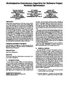
for each i = 1, . . . , m. Under some mild condition [1], for each Pareto-optimal point x∗ , there exists a weight vector λ such that x∗ is the optimal solution of (5), and each optimal solution of (5) is Pareto-optimal to (1). To obtain a set of different Pareto-optimal solutions of (1), one can solve a set of single-objective optimization problems with different weight vectors defined by (4) and (5) or any other decomposition approaches. III. N EW P ROPOSAL : MOEA/D-ACO This section describes the MOEA/D-ACO and its implementations for the MOKP and MTSP. A. Algorithmic Framework MOEA/D-ACO first decomposes the MOP into N singleobjective subproblems by choosing N weight vectors λ1 , . . . , λN . Subproblem i is associated with weight vector λi , and its objective function is denoted as g(x|λi ). MOEA/D-ACO employs N ants for solving these single-objective subproblems. Ant i is responsible for subproblem i. Because g(x|λ) is a continuous function of λ, two subproblems are likely to have similar solutions if their weight vectors are close. Motivated by this observation, MOEA/D-ACO has the following concept. • Neighborhood: The neighborhood B(i) of ant i contains T ants whose subproblem’s weight vectors are the T closest to λi among all the N weight vectors. We always assume that i ∈ B(i); in other words, ant i is its own neighbor. In addition, MOEA/D-ACO introduces the group concept. • Group: The N ants are divided into K groups by clustering their corresponding weight vectors. Each group is intended to approximate a small range of the PF. Fig. 1 illustrates the ideas of decomposition, neighborhoods, and groups in MOEA/D-ACO. To the best of our knowledge, the group concept was first used in BicriterionAnt [24] for biobjective optimization. BicriterionAnt is a Pareto-dominance based method, whereas MOEA/D-ACO adopts a decomposition approach. 3 In

the case of maximization, zi∗ = maxx∈Ω fi (x).

1848


Fig. 1. In this illustrative example, the number of objectives (i.e., m) is 2, the number of ants (i.e., N ) is 14, the number of groups (i.e., K) is 2, and the neighborhood size (i.e., T ) is 5, The MOP is decomposed into 14 single-objective subproblems. Ant i is responsible for finding the optimal solution of subproblem i. Group 1 contains ant 1, 2, . . ., 7, and Group 2 contains ant 8, 9, . . ., 14. Each ant has five neighbors (including itself). As shown in this figure, the neighbors of ant 6 are ants 4, 5, 6, 7, and 8.

At each generation, MOEA/D-ACO with N ants maintains the following: • N solutions x1 , . . . , xN ∈ Ω, where xi is the current solution to subproblem i; • F 1 , . . . , F N , where F i is the F -value of xi , i.e., F i = F (xi ); • τ 1 , . . . , τ K , where τ j is the current pheromone matrix for group j, storing its learned knowledge about the subregion of the PF that it aims at approximating; • η 1 , . . . , η N , where η i is the heuristic information matrix for subproblem i, which is predetermined before the search; • EP , which is the external archive containing all the nondominated solutions found so far. MOEA/D-ACO works as follows: Step 0 Initialization: For i = 1, . . . , N , generate initial solution xi to subproblem i and set F i = F (xi ). For i = 1, . . . , N , initialize η i , the heuristic information matrix to subproblem i. For j = 1, . . . , K, initialize pheromone information matrix τ j for group j. Initialize EP as the set of all the nondominated vectors in {F 1 , . . . , F N }. Step 1 Solution Construction: For each i = 1, . . . , N , ant i constructs a new solution y i by using a probabilistic rule to choose solution components. The rule is a function of xi , η i , and τ j , where ant i is in group j. Compute F (y i ). Step 2 Update of EP : For each i = 1, . . . , N , if no vector in EP dominates F (y i ), add F (y i ) to EP and remove from EP all the vectors dominated by F (y i ). Step 3 Termination: If a problem-specific stopping condition is met, stop and output EP .

Step 4 Update of Pheromone Matrices: For each j = 1, . . . , K, update pheromone matrix τ j by using information extracted from those new solutions that were constructed by ants in group j in Step 1 and have just been added to EP in Step 2. Step 5 Update of xi : For i = 1, . . . , N , ant i finds y, i.e., the solution with the smallest g(·|λi ) value among all the new solutions that were constructed by its neighbors and have not been used to replace any other old solutions; replace xi by y if g(y|λi ) < g(xi |λi ). Go to Step 1. At each generation, each ant constructs a solution in Step 1. These newly constructed solutions update the external archive in Step 2. An ant updates the pheromone matrix of its group in Step 4 if it has found a new nondominated solution. In Step 5, each ant updates its current solution if there is a solution that: 1) is better than its current solution; 2) has not been used for updating other old solutions; and 3) was generated by its neighbors. Step 3 is termination. MOEA/D-ACO is an anytime algorithm; it is always able to return complete and feasible solutions. In the above top-level description, the details of some steps are problem specific. In the following, we take the MOKP and MTSP as examples to show how these steps can be implemented. We would like to point out that our implementation is not unique. There are many possible ways to instantiate the above framework. B. MOEA/D-ACO for the MOKP 1) Basic Setting: • Setting of N and λ1 , . . . , λN : This is controlled by parameter H. More precisely, λ1 , . . . , λN are all the weight


vectors in which each individual weight component takes a value from 0 1 H , ,..., . H H H Therefore, the number of the weight vectors is m−1 . N = CH+m−1

where τkj can be interpreted as a figure of merit, which is learned from the previous search, to measure the benefit of xk = 1 in a solution for the task of group j. The heuristic information matrix for ant i is η i = η1i , . . . , ηni where ηki is to measure the desirability, learned from the domain knowledge before the search, that xk = 1 in a solution for subproblem i. 2) Initialization: • The value of the kth element in η i , the heuristic information matrix for ant i, is set as m i l=1 λl pl,k (8) ηki = m i l=1 γl wl,k where γli is the shadow price of constraint l in the linear programming relaxation of (4) with weight vector λi . ηki is the pseudoutility ratio [50], which has been used as a heuristic information value in [51]. • All the pheromone values are initialized to be the same large value. In our experiments, we have =1

3) Solution Construction: Assume that ant i is in group j and that its current solution is xi = (xi1 , . . . , xin ). In Step 1 of MOEA/D-ACO, ant i constructs a new solution y i = (y1i , . . . , yni ) as follows. 1. For k = 1, . . . , n, set α β ηki φk = τkj + Δ × xik (10)

(7)

• Setting of Group: K representative weight vectors ξ 1 , . . . , ξ K are generated by using the same method as above with a smaller value of H. Then, we cluster λ1 , . . . , λN into K groups so that ξ i is the closest representative vector, in terms of Euclidean distance, to all the weight vectors in group i. • Setting of Neighborhood: The Euclidean distance is used to compute the distance between any two weight vectors. • Decomposition Approach: Both the weighted sum and Tchebycheff approaches are used in this paper. In the Tchebycheff approach, the reference point z ∗ is substituted by z = (z1 , . . . , zm ), where zi is the best value of function fi found so far. • The Data Structure of Pheromone and Heuristic Information Matrices: Because each candidate solution to the MOKP is an n-Dimensional 0–1 vector, we represent pheromone and heuristic information matrices by using n-dimensional real-valued vectors. More precisely, the pheromone matrix for group j is τ j = τ1j , . . . , τnj

τkj

1849

(9)

for all j = 1, . . . , K and k = 1, . . . , n. The motivation is to encourage the search to focus on exploration at its early stage.

where Δ, α, and β > 0 are three control parameters. φk represents the desirability that yki = 1 in y i (i.e., item k is selected) for subproblem i. 2. Initialize y i = (0, . . . , 0) (i.e., the knapsack is empty). Set I = {1, . . . , n}. Do while I = ∅: 2.1 For each s ∈ I, remove s from I if setting ysi = 1 (i.e., adding s to the knapsack) will make y i infeasible. 2.2 If I = ∅, return y i . 2.3 Generate a uniformly random number from (0, 1). If it is smaller than a control parameter r, set s to be the index in I with the largest φ value; otherwise, select one index s randomly from I according to the following probability by the roulette wheel selection:

φs k∈I

φk

.

2.4 Remove s from I and set ysi = 1. In (10), τkj is the pheromone trail of item k shared by all the ants in group j. xik = 1 means that item k is selected in the current solution of subproblem i. xik is private to ant i. Thus, τkj + Δ × xik is a combination of the group and private knowledge. This combination can be regarded as a private pheromone trail of item k for ant i. As in other ACO algorithms, α and β are for balancing the contributions from the pheromone trails and heuristic information values. In Step 2.3, the selection of s follows the so-called pseudorandom proportional rule [13]. The control parameter r is used to balance exploration and exploitation. If the generated random number is smaller than r, the ant does exploitation and selects the item with the largest desirability; otherwise, it conducts random exploration biased toward items with large desirability. 4) Update of Pheromone Matrices: Let Π be the set of all the new solutions: • that were constructed by the ants in group j in Step 1 of the current iteration; • that were just added to EP in Step 2; • in which xk = 1. τkj , i.e., the pheromone trail value of item k for group j, is updated as follows: 1 m n (11) τkj := ρτkj + j i=1 j=1 pij − g(x|λ ) x∈Π

where ρ is the persistence rate of the old pheromone trails. With this update scheme, pheromone matrix τ j stores some statistical information of good solutions found so far for the task of group j. To avoid abnormally large or small pheromone trails, the upper and lower bounds of pheromone values τmax and

1850


τmin are used to limit the range of pheromone trails in our implementation. Following the max–min ant system [14], MOEA/D-ACO, at each generation, updates τmax as follows: τmax =

(1 − ρ)

B+1 n

m i=1

j=1 pij − gmax

(12)

where B is the number of nondominated solutions found at the current iteration, and gmax is the largest value obtained for the objectives functions of all the N subproblems. τmin is always set as τmin = ετmax

(13)

where 0 < ε < 1 is a control parameter. Then, for τkj obtained in (11), reset τkj = τmin if τkj < τmin , and reset τkj = τmax if τkj > τmax . C. MOEA/D-ACO for the MTSP 1) Basic Setting: It is the same as that for the MOKP, except the data structures of pheromone and heuristic information matrices, and solutions are as follows. j • Each group j has pheromone trail τk, l for a link between two different cities k and l. i • Each ant i has a heuristic information value ηk, l for a link between cities k and l. • Each individual solution x is a tour represented by permutation. 2) Initialization: Heuristic information values are initialized as i ηk, l = m

1

j=1

λij cjk, l

.

(14)

k Similar to the implementation for the MOKP, τi,j is initialized to 1. 3) Solution Construction: Assume that ant i is in group j, and its full-scale current solution xi = (xi1 , . . . , xin ). In Step 1 of MOEA/D-ACO, ant i constructs its new solution y i = (y1i , . . . , yni ) as follows. 1. For k, l = 1, . . . , n, set

i i α i β φk, l = τk, ηk, l (15) l + Δ × In x , (k, l)

where Δ, α, and β > 0 are three control parameters. φk, l represents the attractiveness of the link between cities k and l to ant i. The indicator function In(xi , (k, l)) is equal to 1 if link (k, l) is in tour xi or 0 if otherwise. 2. Ant i first randomly selects a city as its starting point and then builds its tour city by city. Suppose that its current position is l and it has not completed its tour. It chooses city k to visit next from C, i.e., the set of the cities not visited so far, as follows: Do while there are unvisited cities: 2.1 Generate a uniformly random number from (0, 1). If it is smaller than a control parameter r, choose k to be the city in C with the largest φ value; otherwise,

select k randomly from C according to the following probability by the roulette wheel selection:

φk, l . s∈C φs, l

2.2 If the ant has visited all the cities, return its tour. 4) Update of Pheromone Matrices: Let Π be the set of all the new solutions that: • were constructed by the ants in group j in Step 1 of the current iteration; • were just added to EP in Step 2; • contain the link between cities k and l. j τk, l , i.e., the pheromone trail value of link (k, l) for group j, is updated as follows: j j τk, l := ρτk, l +

x∈Π

1 g(x|λj )

(16)

where ρ is the persistence rate of the old pheromone trails. As in the implementation for the MOKP, τmax and τmin are used to limit the range of pheromone trails in our implementation. At each generation, τmax is set: τmax =

B+1 (1 − ρ)gmin

(17)

where B is the number of nondominated solutions found at the current iteration, and gmin is the smallest value obtained for the objectives functions of all the N subproblems. τmin is τmin = ετmax

(18)

j where 0 < ε < 1 is a control parameter. Then, for τk, l obtained j j j in (16), reset τk, l = τmin if τk, l < τmin , and τk, l = τmax if j τk, l > τmax .

IV. C OMPARISON W ITH MOEA/D-GA ON THE MOKP In [25], an implementation of MOEA/D with conventional genetic operators and local search (denoted by MOEA/D-GA in the following) is proposed for the MOKP. The crossover operator used is the one-point crossover and the mutation operator mutates each position of a solution with a very low probability. The local search used in MOEA/D-GA was developed by Jaszkiewicz [28]. The major reasons for this comparison are twofold: First, MOEA/D-GA outperforms some other popular and efficient EAs, such as MOGLS on the MOKP [28], and second, both MOEA/D-GA and MOEA/D-ACO use the MOEA/D framework. This comparison is necessary for studying the effect of using ACO in MOEA/D. A. Experimental Setup The nine instances from [3] are used in our experiments. The parameter setting in MOEA/D-GA is the same as in [25], which demonstrated that the weighted sum approach performs


TABLE I T HE S ETTINGS OF THE N UMBER OF A NTS , N (H), AND THE N UMBER OF G ROUPS , K(H), IN MOEA/D-ACO FOR THE MOKP

much better than the Tchebycheff approach in MOEA/D-GA for the MOKP. In our comparison, MOEA/D-GA uses the weighted sum approach as its decomposition approach. To make a fair comparison, the parameters with respect to the MOEA/D framework in MOEA/D-ACO are the same as those in MOEA/D-GA. Both the weighted sum and Tchebycheff approaches are tested in MOEA/D-ACO. The settings of the number of ants and the number of groups for all instances are given in Table I. The other parameters are set as follows. • T = 10. • α = 1. • β = 10. • ρ = 0.95. • r = 0.9. • ε = (1/2n). • Δ = 0.05 × τmax . Both algorithms stop after 300 generations. All the experiments have been carried out on the same computer (a Pentium IV 3-GHz CPU and 2 GB RAM). The programming language is C++. All the statistics are based on 30 independent runs. B. Performance Metric The inverted generational distance (IGD) [25] is used in assessing the performance of the algorithms in our experimental studies. Let P ∗ be a set of uniformly distributed points in the objective space along the PF. Let P be an approximation to the PF, the IGD from P ∗ to P is defined as ∗ d(v, P ) ∗ D(P , P ) = v∈P ∗ |P | where d(v, P ) is the minimum Euclidean distance between v and the points in P . If P ∗ is large enough to represent the PF very well, D(P ∗ , P ) measures both the diversity and convergence of P . To have a low value of D(P ∗ , P ), P must be very close to the PF and cannot miss any part of the whole PF. We chose the upper approximations obtained by Jaszkiewicz [28] as P ∗ in our experiments on the MOKP. C. Comparison Results Table II presents the mean and standard deviation of the IGD values of the final approximations obtained by each algorithm

1851

TABLE II T HE IGD S TATISTICS OF THE F INAL A PPROXIMATIONS O BTAINED BY MOEA/D-ACOW , MOEA/D-ACOT , AND MOEA/D-GA

TABLE III AVERAGE CPU T IME ( IN S ECONDS ) U SED BY MOEA/D-ACOW , MOEA/D-ACOT , AND MOEA/D-GA

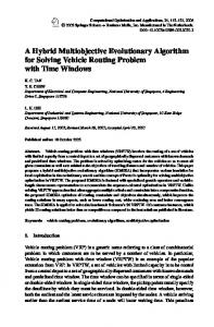
among 30 runs for each test instance. Table III shows the average CPU time used by each algorithm. Fig. 2 plots the distribution of the final approximation with the lowest IGD value among 30 runs of each algorithm for each biobjective test instance. MOEA/D-ACOW and MOEA/D-ACOT represent MOEA/D-ACO with the weighted sum approach and the Tchebycheff approach, respectively. Figs. 3–5 show the evolution of the mean of the IGD value with the number of generations. It is clear from Table II that the final approximations obtained by both variants of MOEA/D-ACO are much better than those obtained by MOEA/D-GA in terms of the IGD metric value on all the test instances. For example, the average IGD values in both MOEA/D-ACO variants are about 23%, 22%, and 25% of those obtained by MOEA/D-GA on instances 250-2, 500-3, 750-4, respectively. From these figures, it is also clear that the differences in the final approximations between two MOEA/D-ACO variants are very small and therefore difficult to distinguish visually. It is evident in Fig. 2 that almost all the final solutions with the lowest IGD values obtained by MOEA/D-GA are dominated by those obtained by MOEA/D-ACO variants on instances 250-2, 500-2, and 750-2. Clearly, the larger the number of decision variables is, the larger the difference between MOEA/D-ACO and MOEA/D-GA is. Table III suggests that both MOEA/D-ACO variants consume more CPU time than MOEA/D-GA. This should be because the ACO component involves more computational overhead than crossover and mutation operators. When concentrating the attention on function evaluations, i.e., the number of candidate solutions visited, Figs. 3–5 indicate that both MOEA/D-ACO variants are always more efficient in terms of the number of function evaluations than MOEA/D-GA in minimizing the IGD values on all the

1852


Fig. 2. Final approximations with the lowest IGD value among 30 runs obtained by MOEA/D-ACOW , MOEA/D-ACOT , and MOEA/D-GA on instance 250-2, 500-2, and 750-2. In each subplot, the horizontal and longitudinal axes correspond to the first and second objective functions, respectively.

three biobjective test instances. The final IGD values obtained by MOEA/D-GA are larger than the final IGD values obtained by MOEA/D-ACO variants. D. More Discussions Both MOEA/D-ACO and MOEA/D-GA adopt the same MOEA/D framework. Therefore, the success of MOEA/DACO should therefore be credited to its ACO part. A distinct feature of ACO is that it makes good use of the heuristic information matrices and uses them to guide its solution construction. From (10), β = 0 in MOEA/D-ACO means that the

heuristic information will make no contribution to solution construction. To investigate the effect of the heuristic information matrices on the performance of MOEA/D-ACO, we have set β = 0 and kept all the other parameters the same as in Section IV-A, and tested MOEA/D-ACO on all the MOKP instances. The IGD statistics of 30 independent runs obtained by MOEA-ACO variants without heuristic information are presented and compared in Table IV. Clearly, MOEA/D-ACO variants without heuristic information performs much poorer than those with heuristic information on all the instances. For example, on instance 250-2, the average IGD-value obtained by MOEA/D-ACOW without heuristic information is about


1853

Fig. 3. Evolution of average IGD values with the number of generations in instance 250-2. In each subplot, the horizontal and longitudinal axes correspond to the number of generations and the average IGD value, respectively.



79 times as large as that obtained with heuristic information. Comparing the results in Tables II and IV, one can find that MOEA/D-ACO variants without heuristic information are also poorer than MOEA/D-GA on all the instances. Thus, one can claim that the use of heuristic information significantly improves the performance of MOEA/D-ACO. As it is the case for most heuristic approaches, ACO is not a black-box method, it requires intuition and intelligence of designers to be embodied into the heuristic information matrix for achieving good performance.

V. C OMPARISON W ITH B ICRITERIONA NT ON THE MTSP BicriterionAnt [24] is one of the best existing mACOs on the biobjective TSP [19], [22]. As pointed out in the introduction, BicriterionAnt also uses the group concept. It relies on Pareto dominance for guiding its search, whereas MOEA/D-ACO employs decomposition for dealing with MOPs. Both of them use ACO approaches for constructing new solutions. Therefore, this comparison should be useful for understanding the benefit of the decomposition approach.

1854


TABLE IV IGD S TATISTICS O BTAINED BY MOEA/D-ACO FOR S TUDYING THE I NFLUENCE OF H EURISTIC I NFORMATION

TABLE V T HE IGD S TATISTICS OF THE F INAL A PPROXIMATIONS O BTAINED BY MOEA/D-ACOW , MOEA/D-ACOT , AND B ICRITERIONA NT

A. Experimental Setup

B. Experimental Results

The 12 instances from [52] are used in the comparison. The parameter setting of BicriterionAnt is the same as in [22]. Specifically, we have the following.

Table V shows that the IGD values of the final approximations obtained by both MOEA/D-ACO variants are nearly one order of magnitude lower than those by BicriterionAnt on all test instances. However, there is no substantial difference between two MOEA/D-ACO variants in terms of the IGD value. In Fig. 6, the quality differences between each MOEA/D-ACO variant and BicriterionAnt can be visually detected. Clearly, the final solutions obtained by MOEA/D-ACO variants dominate almost all the final solutions found by BicriterionAnt. Figs. 7–9 suggest that both MOEA/D-ACO are more efficient in reducing the IGD values than BicriterionAnt. These experimental results indicate that the MOEA/D framework does indeed help to improve the algorithm performance. The major reason could be that the decomposition strategy makes cooperation among different ants more efficient than Pareto dominance. It is also clear in Figs. 7–9 that MOEA/D-ACOT performs better than MOEA/D-ACOW . Table VI shows that both MOEA/D-ACO variants require much less CPU time than BicriterionAnt. This is because BicriterionAnt needs to compare all the solutions to each other at each generation, which is very time-consuming.

• • • • • •

number of groups = 3. number of ant in each group = 8. ρ = 0.95. α = 1. β = 2. r = 0.9.

The parameter settings of MOEA/D-ACO are as follows. • • • • • • • • •

Total number of ants N = 24. Number of groups K = 3. Neighborhood size T = 10. ρ = 0.95. α = 1. β = 2. r = 0.9. = (1/2n). Δ = 0.05 × τmax .

In computing the IGD values, P ∗ for each instance is the set of all the nondominated solutions found by all the runs of all the algorithms. Both algorithms stop after 3000 generations. Therefore, they construct the same number of candidate solutions for each instance. All statistics are based on 30 independent runs.

C. More Discussions Both MOEA/D-ACO and BicriterionAnt use ACO for solution construction. Unlike BicriterionAnt, each ant in MOEA/DACO records its current solution and uses it to compute φk in


1855

Fig. 6. Final approximations with the lowest IGD value among 30 runs obtained by two MOEA/D-ACO variants and BicriterionAnt on instance krode100, kroab200, and kroab300. In each subplot, the horizontal and longitudinal axes correspond to the first and second objective functions, respectively.

(15) for solution construction. MOEA/D-ACO also uses groups and neighborhoods to allow ants to exchange information. Thus, three issues arise naturally. • What if grouping is not used in MOEA/D-ACO? • What if the current solution makes no contribution to φk in (15) in MOEA/D-ACO? • What if individual ants do not change information with their neighbors as described in Step 5 in MOEA/D-ACO? Noting that K = 1 implies that no grouping is used, Δ = 0 means that the current solution makes no contribution, and

T = 1 means that an ant has no neighbor except itself, we tested MOEA/D-ACO variants in which K = 1, Δ = 0, or T = 1, whereas the other parameters are the same as in Section V-A. The experimental results are listed in Tables VII and VIII, from which we can observe the following. • Both MOEA/D-ACO variants with grouping (i.e., the default parameter setting) significantly outperform their counterparts without grouping. For example, in kroab200, the IGD value of MOEA/D-ACOW with grouping is about 80% of that obtained without grouping.

1856


Fig. 7. Evolution of average IGD values with the number of generations in instance krode100. In each subplot, the horizontal and longitudinal axes correspond to the number of generations and the average IGD value, respectively.

Fig. 8. Evolution of average IGD values with the number of generations in kroab200. In each subplot, the horizontal and longitudinal axes correspond to the number of generations and the average IGD value, respectively.

Fig. 9. Evolution of average IGD values with the number of generations in kroab300. In each subplot, the horizontal and longitudinal axes correspond to the number of generations and the average IGD value, respectively.

• Both MOEA/D-ACO variants with the default parameter setting are significantly better than those with Δ = 0 on all the 12 test instances. Taking kroab100 as an example, the IGD value of MOEA/D-ACOT with the default parameter setting is about 78% of that obtained without using location information of the current solutions. • Both MOEA/D-ACO variants with the default parameter setting significantly outperform their counterparts with T = 1 on all test instances.

Therefore, one can claim that grouping, the location information of the current solutions, and the neighborhood significantly improve the algorithm performance. In our experiments, there is no instance in which these techniques cause any deterioration. VI. C ONCLUSION AND F UTURE R ESEARCH I SSUES Reactive search optimization principle, i.e., “learning while optimizing,” has been widely used for designing and improving metaheuristics [11]. ACO is a successful heuristic using this


1857

TABLE VI AVERAGE RUNNING T IME ( IN S ECONDS ) C ONSUMED BY MOEA/D-ACO AND B ICRITERIONA NT

TABLE VII T HE IGD S TATISTICS OF THE F INAL A PPROXIMATIONS O BTAINED BY MOEA/D-ACOW W HEN K = 1, Δ = 0, AND T = 1

TABLE VIII T HE IGD S TATISTICS OF THE F INAL A PPROXIMATIONS O BTAINED BY MOEA/D-ACO T W HEN K = 1, Δ = 0, AND T = 1

principle. ACO for single-objective optimization represents its problem specific knowledge as a heuristic information matrix and its knowledge learned from the previous search as a pheromone matrix. Because the goal of multiobjective optimization is to approximate the PF, instead of a single optimal solution, generalizing ACO to multiobjective optimization is not a trivial task. MOEA/D decomposes an MOP into a number of singleobjective subproblems and optimizes them simultaneously. Neighborhood relations among these subproblems are defined and used to make the search efficient and effective. With the MOEA/D framework, this paper designed an mACO, i.e.,

MOEA/D-ACO. In this proposed algorithm, each ant is responsible for one subproblem. The ants are divided into groups, and each ant has several neighboring ants. An ant group maintains a pheromone matrix, and an individual ant has a heuristic information matrix. During the search, each ant also records the best solution found so far for its subproblem. To construct a new solution, an ant combines information from its group’s pheromone matrix, its own heuristic information matrix and its current solution. We conducted extensive experimental results on two paradigmatic MOPs. The experimental results on the MOKP show that MOEA/D-ACO outperforms MOEA/D-GA on all the nine

1858


test instances. Furthermore, the heuristic information matrices in MOEA/D-ACO make a very significant contribution to its performance. In other words, MOEA/D-ACO successfully inherits the learning and adaptation ability of single-objective ACO. The comparison of MOEA/D-ACO with BicriterionAnt, which is a very efficient mACO proposed in the previous literature, on the biobjective TSP has shown that MOEA/DACO performs much better on all the 12 test instances. We also studied the effects of grouping, the neighborhood, and the use of location information of current solutions on the performance of MOEA/D-ACO. We believe that our proposed hybrid approach can be extended in several ways. The future research avenues include the following. • The studies of MOEA/D-ACO on other hard or real-world multiobjective problems. Specific attention should be paid for how to decompose these MOPs and how to define their heuristic information and pheromone matrices. • The investigation of online parameter-tuning and configuration techniques in MOEA/D-ACO. Although the manual tuning in this paper provided excellent results, it is worthwhile studying automatic tuning techniques based on machine learning for extending MOEA/D-ACO to different problems [11], [53]. • The combinations of MOEA/D-ACO with single objective search techniques. Although MOEA/D framework provides a very natural framework for using single-objective search techniques, it is worthwhile studying when and how single-objective search techniques can be used in MOEA/D-ACO. • The use of MOEA/D-ACO in two-phase Pareto search. A two-phase strategy first generates a set of high-quality solutions by a search method and then applies Pareto local search on them to generate approximate Pareto-optimal solutions [54]. It is very interesting to study how to use MOEA/D-ACO in the first phase. • The use of the ideas in MOEA/D-ACO for generating EDAs to multiobjective optimization. Hybrids of EDAs with other techniques have been widely studied and used for single-objective optimization (e.g., in [55] and [56]). These experiences should be very useful for combining MOEA/D with EDA. • The studies of combination of MOEA/D-ACO with the DM’s preference information. The brain–computer evolutionary multiobjective optimization scheme approximates a utility function in an interactive manner [57] for reducing the cognitive burden on the DM. It is very interesting to study how the DM’s preference can be integrated into MOEA/D-ACO in such a way. The C++ source code of MOEA/D-ACO can be downloaded from Qingfu Zhang’s homepage: http://dces.essex.ac.uk/staff/ qzhang/. ACKNOWLEDGMENT The authors would like to thank the anonymous reviewers and the associate editor.

R EFERENCES [1] K. Miettinen, Nonlinear Multiobjective Optimization. Boston, MA: Kluwer, 1999. [2] K. Deb, S. Agrawal, A. Pratap, and T. Meyarivan, “A fast and elitist multiobjective genetic algorithm: NSGA-II,” IEEE Trans. Evol. Comput., vol. 6, no. 2, pp. 182–197, Apr. 2002. [3] E. Zitzler and L. Thiele, “Multiobjective evolutionary algorithms: A comparative case study and the strength Pareto approach,” IEEE Trans. Evol. Comput., vol. 3, no. 4, pp. 257–271, Nov. 1999. [4] K. Deb, Multi-Objective Optimization Using Evolutionary Algorithms. New York: Wiley, 2001. [5] C. A. C. Coello, D. A. V. Veldhuizen, and G. B. Lamont, Evolutionary Algorithms for Solving Multi-Objective Problems. Norwell, MA: Kluwer, May 2002. [6] K. Tan, E. Khor, and T. Lee, Multiobjective Evolutionary Algorithms and Applications. Berlin, Germany: Springer-Verlag, 2005, ser. Advanced Information and Knowledge Processing. [7] J. Knowles and D. Corne, “Memetic algorithms for multiobjective optimization: Issues, methods and prospects,” in Recent Advances in Memetic Algorithms. Heidelberg, Germany: Springer-Verlag, 2004, pp. 313–352. [8] Q. Zhang, A. Zhou, and Y. Jin, “RM-MEDA: A regularity model based multiobjective estimation of distribution algorithm,” IEEE Trans. Evol. Comput., vol. 12, no. 1, pp. 41–63, Feb. 2008. [9] P.-C. Chang and S.-H. Chen, “The development of a sub-population genetic algorithm II (SPGA II) for multi-objective combinatorial problems,” Appl. Soft Comput., vol. 9, no. 1, pp. 173–181, Jan. 2009. [10] R. Battiti and G. Tecchiolli, “The reactive tabu search,” ORSA J. Comput., vol. 6, no. 2, pp. 126–140, Spring 1994. [11] R. Battiti, M. Brunato, and F. Mascia, Reactive Search and Intelligent Optimization. Berlin, Germany: Springer-Verlag, 2008, ser. Operations Research/Computer Science Interfaces. [12] M. Dorigo, V. Maniezzo, and A. Colorni, “Ant system: Optimization by a colony of cooperating agents,” IEEE Trans. Syst., Man, Cybern. B, Cybern., vol. 26, no. 1, pp. 29–41, Feb. 1996. [13] M. Dorigo and L. Gambardella, “Ant colony system: A cooperative learning approach to the travelling salesman problem,” IEEE Trans. Evol. Comput., vol. 1, no. 1, pp. 53–66, Apr. 1997. [14] T. Stützle and H. Hoos, “Max-min ant system,” Future Gener. Comput. Syst., vol. 16, no. 9, pp. 889–914, Jun. 2000. [15] B. Bullnheimer, G. Kotsis, and C. Strauss, “A new rank-based version of the ant system: A computational study,” Central Eur. J. Oper. Res., vol. 7, no. 1, pp. 25–38, Jan. 1999. [16] O. Cordon, I. F. de Viana, and F. Herrera, “Analysis of the best-worst ant system and its variants on the TSP,” Math. Soft Comput., vol. 9, no. 2/3, pp. 177–192, 2002. [17] M. Dorigo and T. Stützle, Ant Colony Optimization. Cambridge, MA: MIT Press, 2004. [18] K. Doerner, W. J. Gutjahr, R. F. Hartl, C. Strauss, and C. Stummer, “Pareto ant colony optimization: A metaheuristic approach to multiobjective portfolio selection,” Ann. Oper. Res., vol. 131, no. 1–4, pp. 79–99, Oct. 2004. [19] C. Garcia-Martinez, O. Cordon, and F. Herrera, “A taxonomy and an empirical analysis of multiple objective ant colony optimization algorithms for the bi-criteria TSP,” Eur. J. Oper. Res., vol. 180, no. 1, pp. 116–148, Jul. 2007. [20] D. Angus and C. Woodward, “Multiple objective ant colony optimization,” Swarm Intell., vol. 3, no. 1, pp. 69–85, 2009. [21] I. Alaya, C. Solnon, and K. Ghedira, “Ant colony optimization for multiobjective optimization problems,” in Proc. 19th IEEE Int. Conf. Tools Artif. Intell., 2007, pp. 450–457. [22] M. López-Ibáñez and T. Stützle, “The impact of design choices of multiobjective ant colony optimization algorithms on performance: An experimental study on the biobjective TSP,” in Proc. GECCO, 2010, pp. 71–78. [23] M. Guntsch and M. Middendorf, “A population based approach for aco applications of evolutionary computing,” in Proc. Appl. Evol. Comput. EvoWorkshops––EvoCOP, EvoIASP, EvoSTIM/EvoPLAN, 2002, pp. 72–81. [24] S. Iredi, D. Merkle, and M. Middendorf, “Bi-criterion optimization with multi colony ant algorithms,” in Proc. 1st Int. Conf. EMO, 2001, pp. 359–372. [25] Q. Zhang and H. Li, “MOEA/D: A multiobjective evolutionary algorithm based on decomposition,” IEEE Trans. Evol. Comput., vol. 11, no. 6, pp. 712–731, Dec. 2007. [26] H. Ishibuchi and T. Murata, “Multi-objective genetic local search algorithm and its application to flowshop scheduling,” IEEE Trans. Syst., Man, Cybern. C, Appl. Rev., vol. 28, no. 3, pp. 392–403, Aug. 1998.


[27] H. Ishibuchi and Y. Shibata, “An empirical study on the effect of mating restriction on the search ability of EMO algorithms,” in Proc. EMO, 2003, pp. 433–447. [28] A. Jaszkiewicz, “On the performance of multiple-objective genetic local search on the 0/1 knapsack problem—A comparative experiment,” IEEE Trans. Evol. Comput., vol. 6, no. 4, pp. 402–412, Aug. 2002. [29] E. J. Hughes, “Multiple single objective Pareto sampling,” in Proc. IEEE CEC, 2003, pp. 2678–2684. [30] Y. Jin, T. Okabe, and B. Sendhoff, “Adapting weighted aggregation for multiobjective evolution strategies,” in Proc. 1st Int. Conf. EMO, Zurich, Switzerland, 2001, vol. 1993, pp. 96–110, ser. LNCS. [31] H. Ishibuchi, Y. Sakane, N. Tsukamoto, and Y. Nojima, “Adaptation of scalarizing functions in MOEA/D: An adaptive scalarizing function-based multiobjective evolutionary algorithm,” in Proc. EMO, Berlin, Germany, 2009, vol. 5467, pp. 438–452, Lecture Notes in Computer Science. [32] H. Ishibuchi, Y. Sakane, N. Tsukamoto, and Y. Nojima, “Evolutionary many-objective optimization by NSGA-II and MOEA/D with large populations,” in Proc. IEEE Int. Conf. Syst., Man, Cybern., San Antonio, TX, 2009, pp. 1758–1763. [33] H. Ishibuchi, Y. Sakane, N. Tsukamoto, and Y. Nojima, “Simultaneous use of different scalarizing functions in MOEA/D,” in Proc. GECCO, Portland, OR, 2010, pp. 519–526. [34] S. Pal, S. Das, A. Basak, and P. N. Suganthan, “Synthesis of difference patterns for monopulse antennas with optimal combination of array-size and number of subarrays—A multi-objective optimization approach,” Progr. Electromagn. Res. B, vol. 21, pp. 257–280, 2010. [35] A. Nebro and J. Durillo, “A study of the parallelization of the multiobjective metaheuristic MOEA/D,” in Proc. LION, Trento, Italy, 2010, pp. 303–317. [36] I. Guerra-Gomez, E. Tlelo-Cuautle, T. McConaghy, and G. Gielen, “Decomposition-based multi-objective optimization of second-generation current conveyors,” in Proc. 52nd IEEE Int. Midwest Symp. Circuits Syst., Cancun, Mexico, 2009, pp. 220–223. [37] Y.-H. Chan, T.-C. Chiang, and L.-C. Fu, “A two-phase evolutionary algorithm for multiobjective mining of classification rules,” in Proc. IEEE CEC, Barcelona, Spain, 2010, pp. 1–7. [38] C.-M. Chen, Y. p. Chen, T.-C. Shen, and J. Zhao, “Optimizing degree distributions in LT codes by using the multiobjective evolutionary algorithm based on decomposition,” in Proc. IEEE CEC, Barcelona, Spain, 2010, pp. 1–8. [39] Y. Mei, K. Tang, and X. Yao, “Decomposition-based memetic algorithm for multi-objective capacitated arc routing problem,” IEEE Trans. Evol. Comput., vol. 15, no. 2, pp. 151–165, Apr. 2011. [40] N. A. Moubayed, A. Petrovski, and J. McCall, “A novel smart multiobjective particle swarm optimisation using decomposition,” in Proc. 11th PPSN, Berlin, Germany, 2010, vol. 6239, pp. 1–10, Lecture Notes in Computer Science. [41] B. D. Daz, P. Bouvry, J. A. Canero, A. A. Maciejewski, and H. J. Siegel, “Multi-objective robust static mapping of independent tasks on grids,” in Proc. IEEE CEC, Barcelona, Spain, 2010, pp. 1–8. [42] A. Konstantinidis, C. Charalambous, A. Zhou, and Q. Zhang, “Multiobjective mobile agent-based sensor network routing using MOEA/D,” in Proc. IEEE Congr. Evol. Comput., 2010, pp. 1–8. [43] I. Giagkiozis, R. Purshouse, and P. Fleming, “Generalized decomposition,” in Proc. Evol. Multi-Criterion Optim., Berlin, Germany, 2013, ser. Lecture Notes in Computer Science. [44] V. Shim, K. Tan, and C. Cheong, “A hybrid estimation of distribution algorithm with decomposition for solving the multiobjective multiple traveling salesman problem,” IEEE Trans. Syst., Man, Cybern. C, Appl. Rev., vol. 42, no. 5, pp. 682–691, Sep. 2012. [45] K. Sindhya, K. Miettinen, and K. Deb, “A hybrid framework for evolutionary multi-objective optimization,” IEEE Trans. Evol. Comput., vol. 17, no. 4, pp. 495–511, Aug. 2013. [46] S. Martinez and C. Coello, “A direct local search mechanism for decomposition-based multi-objective evolutionary algorithms,” in Proc. IEEE Congr. Evol. Comput., 2012, pp. 1–8. [47] P. Adriano and S. Paolo, “Scalarizing vector optimization problems,” J. Optim. Theory Appl., vol. 42, no. 4, pp. 499–524, Apr. 1984. [48] M. Ehrgott, Multicriteria Optimization. Berlin, Germany: SpringerVerlag, 2005. [49] G. Eichfelder, Adaptive Scalarization Methods in Multiobjective Optimization. New York: Springer-Verlag, 2008. [50] P. C. Chu and J. E. Beasley, “A genetic algorithm for the multidimensional knapsack problem,” J. Heurist., vol. 4, no. 1, pp. 63–86, Jun. 1998. [51] L. Ke, Z. Feng, Z. Ren, and X. Wei, “An ant colony optimization approach for the multidimensional knapsack problem,” J. Heurist., vol. 16, no. 1, pp. 65–83, Feb. 2010. [52] [Online]. Available: http://eden.dei.uc.pt/~paquete/tsp/

1859

[53] F. Hutter, H. Hoos, and T. Stutzle, “Automatic algorithm configuration based on local search,” in Proc. Nat. Conf. Artif. Intell., 2007, vol. 2, pp. 1152–1157. [54] T. Lust and J. Teghem, “Two-phase Pareto local search for the biobjective traveling salesman problem,” J. Heurist., vol. 16, no. 3, pp. 475–510, Jun. 2010. [55] R. Battiti and M. Brunato, “R-EVO: A reactive evolutionary algorithm for the maximum clique problem,” IEEE Trans. Evol. Comput., vol. 15, no. 6, pp. 770–782, Dec. 2011. [56] Q. Zhang, J. Sun, and E. Tsang, “Evolutionary algorithm with guided mutation for the maximum clique problem,” IEEE Trans. Evol. Comput., vol. 9, no. 2, pp. 192–200, Apr. 2005. [57] R. Battiti and A. Passerini, “Brain-computer evolutionary multi-objective optimization (BC-EMO): A genetic algorithm adapting to the decision maker,” IEEE Trans. Evol. Comput., vol. 14, no. 5, pp. 671–687, Oct. 2010. Liangjun Ke received the B.Sc. and M.Sc. degrees in mathematics from Wuhan University, Wuhan, China, in 1998 and 2001, respectively, and the Ph.D. degree in systems engineering from Xi’an Jiaotong University, Xi’an, China, in 2008. From 2011 to 2012, he visited the School of Computer Science and Electronic Engineering, University of Essex, Colchester, U.K. He is currently an Associate Professor with Xi’an Jiaotong University. His main research interests include optimization theory and applications, particularly multiobjective optimization, evolutionary computation, and robust optimization.

Qingfu Zhang (M’01–SM’06) received the B.Sc. degree in mathematics from Shanxi University, Taiyuan, China, in 1984 and the M.Sc. degree in applied mathematics and the Ph.D. degree in information engineering from Xidian University, Xi’an, China, in 1991 and 1994, respectively. From 1994 to 2000, he was with the National Laboratory of Parallel Processing and Computing, National University of Defence Science and Technology, Changsha, China; Hong Kong Polytechnic University, Kowloon, Hong Kong; German National Research Centre for Information Technology (now FraunhoferGesellschaft, Germany); and the University of Manchester Institute of Science and Technology, Manchester, U.K. He is currently a Professor with the School of Computer Science and Electronic Engineering, University of Essex, Colchester, U.K. He is the holder of two patents and is the author of many research publications. His main research interests include evolutionary computation, optimization, neural networks, data analysis, and their applications. Dr. Zhang is an Associate Editor for the IEEE T RANSACTIONS ON E VO LUTIONARY C OMPUTATION and the IEEE T RANSACTIONS ON S YSTEMS , M AN , AND C YBERNETICS -PART B. He is also an Editorial Board Member of three other international journals. The multiobjective evolutionary algorithm based on decomposition, a multiobjective optimization algorithm developed in his group, won the Unconstrained Multiobjective Optimization Algorithm Competition at the Congress of Evolutionary Computation 2009. He was a recipient of the 2010 IEEE T RANSACTIONS ON E VOLUTIONARY C OMPU TATION Outstanding Paper Award.

Roberto Battiti (F’09) received the B.S. and M.S. degrees in physics from the University of Trento, Trento, Italy, in 1985 and the Ph.D. degree in computation and neural systems from the California Institute of Technology, Pasadena, in 1990. He is currently a Professor of computer science with the Department of Information Engineering and Computer Science, University of Trento, where he is currently the Director of the Machine Learning and Intelligent Optimization Laboratory. He is involved in the LIONsolver.com startup. His research interests include parallel computing to algorithms, machine learning and neural networks, and optimization. His current research aims at combining machine learning and optimization, which has led to two research areas: reactive search optimization, and learning and intelligent optimization.