Hindawi Mathematical Problems in Engineering Volume 2018, Article ID 2571380, 21 pages https://doi.org/10.1155/2018/2571380
Research Article A Bee Evolutionary Algorithm for Multiobjective Vehicle Routing Problem with Simultaneous Pickup and Delivery Guiliang Gong and He Xie2 1
,1 Qianwang Deng
,1 Xuran Gong,1 Like Zhang,1 Haibin Wang,2
State Key Laboratory of Advanced Design and Manufacturing for Vehicle Body, Hunan University, Changsha 410082, China CRRC Zhuzhou Institute Co., Ltd., Zhuzhou 412200, China
2
Correspondence should be addressed to Qianwang Deng; deng
[email protected] Received 15 September 2017; Accepted 19 March 2018; Published 19 June 2018 Academic Editor: Nunzio Salerno Copyright © 2018 Guiliang Gong et al. This is an open access article distributed under the Creative Commons Attribution License, which permits unrestricted use, distribution, and reproduction in any medium, provided the original work is properly cited. A new closed-loop supply chain logistics network of vehicle routing problem with simultaneous pickups and deliveries (VRPSPD) dominated by remanufacturer is constructed, in which the customers are originally divided into three types: distributors, recyclers, and suppliers. Furthermore, the fuel consumption is originally added to the optimization objectives of the proposed VRPSPD. In addition, a bee evolutionary algorithm guiding nondominated sorting genetic algorithm II (BEG-NSGA-II) with a two-stage optimization mechanism is originally designed to solve the proposed VRPSPD model with three optimization objectives: minimum fuel consumption, minimum waiting time, and the shortest delivery distance. The proposed BEG-NSGA-II could conquer the disadvantages of traditional nondominated sorting genetic algorithm II (NSGA-II) and algorithms with a two-stage optimization mechanism. Finally, the validity and feasibility of the proposed model and algorithm are verified by simulating an engineering machinery remanufacturing company’s reverse logistics and another three test examples.
1. Introduction Recycling and remanufacturing is an integral system by which the old or discarded products are recycled and then processed, recovered, and sold as like-new ones in the markets [1], and the environmental impacts are also reduced by maintaining the geometrical form of the products, thus preserving its environmental and economic values [2, 3]. It is one of the important ways to realize the green sustainable development [4, 5]. For example, in recent years, China offers subsidies on a range of vehicles such as small- and mediumsized old vehicles, the rural bus, and yellow-sticker vehicles subsidy in its “automotive replacement” policy, to encourage vehicle owners to submit vehicles to officially recognized endof-life vehicle (ELV) dismantlers [6]. Reverse logistics is a central problem of recycling and remanufacturing of waste products [7–9]. Its path planning has a great influence on distribution efficiency and environmental protection efficiency, which usually includes three main models: vehicle routing problem that delivers the goods before pickups, vehicle routing problem that delivers and pickups the goods in a
mixed way, and vehicle routing problem with simultaneous pickups and deliveries (VRPSPD) of the goods, etc. [10]. The model of VRPSPD is better than other ones in environmental protection and saving cost, for it can make full use of the vehicle load space [11]. Therefore, the VRPSPD problem attracts more and more researchers in recent years. The VRPSPD problem was first introduced by Min [12], who developed a solution procedure to solve a public library distribution with two vehicles. Based on a set of covering formulations, Klose et al. [13] implemented a Branch and Price approach for the VRPSPD. Li and Lim [14] proposed a tabu-embedded simulated annealing algorithm which restarted a search procedure from the current best solution after several nonimproving search iterations. Crispim and Brand˜ao [15] proposed a hybrid heuristic algorithm which combined the tabu search with the falling variable field method for solving the vehicle routing problem with backhauls. Ropke and Pisinger [16] designed an adaptive large neighborhood search heuristic composed of a number of competing subheuristics, which improved many of the best known solutions. Montan´e and Galvao [17]
2 used tabu search algorithm and local optimization method for the VRPSPD problem with maximum travel constraint. Based on GLNPSO, a PSO algorithm with multiple social structures, Ai and Kachitvichyanukul [18] developed a new PSO algorithm for VRPSPD. C ¸ atay [19] proposed an ant colony algorithm by employing a new saving-based visibility function and pheromone updating procedure. Mingyong and Erbao [20] solved the VRPSPD problem with time windows and travel constraints by improving the differential evolution algorithm. Wu et al. [21] proposed a hybrid chaotic quantum evolutionary algorithm which successfully reduced the number of vehicles and the distance of the distribution according to the data in the literature [15]. Subramanian et al. [22] proposed a branch-cut-and-price approach for the VRPSPD problem. By combining a local search named variable neighborhood descent algorithm into PSO, Goksal et al. [23] presented a heuristic approach for VRPSPD and improved several best known solutions. By analysing the vehicle load fluctuation characteristics, Zhang et al. [24] designed a heuristic factor and solved the VRPSPD problem with vehicle travel constraints based on an improved ant colony algorithm. Then Zhang et al. [25] studied the VRPSPD with time dependent vehicle routing problems and developed a hybrid algorithm that integrated both ant colony system and tabu search algorithms for solving it. Polat et al. [26] proposed a perturbation based variable neighborhood search heuristic for solving the VRPSPD problem with time limit. Avci and Topaloglu [27] developed a hybrid local search algorithm in which a nonmonotone threshold adjusting strategy is integrated with tabu search and effectively solved the VRPSPD problem with different types of vehicles. With the deterioration of the environment and the enhancement of environmental protection consciousness, the scholars have begun to take the vehicle fuel consumption as one of the optimization objectives in the past two years. Jin and PeiHua [28] used multistarting tabu search algorithm to study the heterogeneous vehicle low-carbon routing problem based on energy consumption and carbon emissions, then proposed a variable domain random search method, and solved the low energy vehicle routing problem about time windows [29]. By analysing the solution space and complexity of fuelconsumption-minimizing capacitated vehicle routing problem (FCM-CVRP) and capacitated vehicle routing problem (CVRP), Wu et al. [30] found that the FCM-CVRP was more difficult to solve, and they proposed a two-phase algorithm to solve it. Considering the factors of road grade, Rao et al. [31] proposed a low-carbon vehicle routing problem model which has capacity constraints and objective of minimum fuel consumption. Ombuki et al. [32] used a multiobjective evolutionary genetic algorithm based on the Pareto sort for the Vehicle Routing Problem with Time Windows (VRPTW), and its two optimization objectives are minimum number of vehicles and shortest delivery distance. Lau et al. [33] took the shortest delivery distance and the shortest travel time as the optimization objectives and used NSGA-II algorithm guided by fuzzy logic for the routing problem with multiple warehouses, multiple customers, and a variety of products. Ba˜nos et al. [34] put forward a model with two objectives of shortest distance and minimum unbalance load, which
Mathematical Problems in Engineering considered the workload of the vehicle, and proposed a hybrid heuristic algorithm composed of genetic algorithm and simulated annealing algorithm for it. Hsueh [35] studied the vehicle routing problem with the objectives of minimizing the sum of the fixed costs and the expected fuel consumption costs. Jemai, Zekri, and Mellouli [36] studied the Multiobjective GA for green vehicle routing problem with different metrics: computation time, traveled distance, emissions volume, generational distance, spacing, entropy, and contribution. Soleiman Chaharlang and Ghaderi [37] proposed a multiobjective nonlinear programming model for the green vehicle routing problem (GVRP), including original and remanufactured products distribution (both delivery and pickup) of end-of-life (EOL) products. Although there is a stream of research on the VRPSPD problem and related algorithms, we find that there are still some important problems which have been overlooked and needed to be solved. It is indicated that the traditional VRPSPD model only considers a single type of customer. However, in a real recycling and remanufacturing system, customers consist of various types, such as distributors, recyclers, and suppliers. In addition, although the optimization objective of fuel consumption has been studied in some models such as FCM-CVRP and CVRP, it has not been considered in the existing literatures with the traditional VRPSPD. However, the fuel consumption is actually a key factor affecting the resource consumption and environmental destruction in VRPSPD. With regard to the overlooked problems mentioned above, in this paper the customers are originally divided into three types which are distributors, recyclers, and suppliers, and a new closed-loop supply chain logistics network of VRPSPD dominated by remanufacturer is constructed, which is more consistent with the actual situation of recycling and remanufacturing. Furthermore, for the purpose of resource saving and environment protection, the fuel consumption is originally added to the optimization objectives of VRPSPD. Besides, inspired by the literature [38], a bee evolutionary algorithm guiding nondominated sorting genetic algorithm II (BEG-NSGA-II) with a two-stage optimization mechanism is originally designed to solve the proposed VRPSPD model with three optimization objectives: minimum fuel consumption, minimum waiting time, and the shortest delivery distance. The optimal solution should meet the travel constraints as well as load constraints. The proposed BEG-NSGA-II could conquer the disadvantages (premature convergence to local solution and low searching efficiency) of the traditional NSGA-II and the disadvantage (inability to gain stable and high quality initial population in the first stage) of the existing algorithms with two-stage optimization mechanism when it is used to solve the problems with rigor constraints. Finally, the validity and feasibility of the proposed model and algorithm are verified by simulating an engineering machinery remanufacturing company’s reverse logistics and another three test examples. The rest of this paper is organized as follows. The proposed VRPSPD model is constructed in the next section. In Section 2, the multiobjective optimization model of the proposed VRPSPD is proposed. In Section 3, the implementation details of the proposed BEG-NSGA-II are presented.
Mathematical Problems in Engineering
3
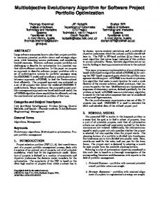
Supplier 1
Distributor 1
Recycling/Remanufacturing company
Supplier 2 .. .
Distributor 2
Recycling center
Distributor 3 .. .
Test
Waste treatment plant
Classify
Disassemble
Supplier n
Distributor n
Recycler 1
Recycler 2
Forward logistics
···
Recycler n
Reverse logistics
Figure 1: The proposed logistics structure.
Afterwards, experimental studies and discussions are made in Section 4. Finally, the conclusions are described in Section 5.
2. The Multiobjective Optimization Model of the Proposed VRPSPD 2.1. The Proposed VRPSPD Model. The proposed VRPSPD model in the paper is shown in Figure 1. This model is described as follows: a group of vehicles start from the recycling and remanufacturing plant with new products; then the vehicles distribute the new products to each distributor, take waste products back from each recycling business, or take new components from supply business during the set time. Some requirements must be met: the load of vehicles with waste products backed from the service points must meet the needs of all distributor points; the load of every service point cannot exceed the allowable values; each service point is serviced only once in a logistics delivery cycle. The following assumptions are made for the network structure: (i) Due to the uncertainty of quantity and quality of recycled products, each service point (except waste treatment plan) in the model should establish an information-sharing platform at the beginning of each logistics cycle; then, according to the information, recycling and remanufacturing factory arranges distribution vehicles. (ii) Distributor points are sale points of remanufacturing products as well as recycling points of waste products. (iii) Recycling process center and recycling and remanufacturing plant are located in the same location. 2.2. Fundamental Assumptions and Parameter Description. The VRPSPD model proposed in this paper is based on the following assumptions: (i) Every vehicle moves at a constant speed between any two customers; namely, the acceleration speed is zero. (ii) Other energy consumption of distribution vehicles (such as air conditioning) is zero, which means Pacc = 0 in (2).
(iii) Every vehicle departs from the recycling company and returns to it in the end. (iv) All vehicles’ maximum payload is identical and they have the same weight as well. (v) The fuel consumption for each vehicle is only affected by three factors, namely, travel distance, payload, and travel speed. (vi) The road slope (𝜃) between any two customers is set to zero, i.e., without considering the road slope of any two customers. By analysing the operating process of recycling and remanufacturing reverse logistics network, recycling points and suppliers can be regarded as special distribution points. So the vehicle routing problem of the proposed model can be changed into VRPSPD. V = {v0 , v1 , v2 , . . ., vn , r1 , r2 , . . .,rm , p1 ,p2 , . . ., ps } is used to express the set of all service points, in which v0 is the recycling and remanufacturing plant, {v1 , v2 , ... vn }is the set of distributors, {r1 , r2 , ..., rm } is the set of recycling points, and {p1 , p2 , ..., ps } is the set of suppliers. Use the corresponding sequence number of each element of V to form a new set 𝑉 ; i.e., 𝑉 = {0, 1, . . ., n, n +1,. . .n + m,. . ., n + m + s}. The parameters used in the definition of multiobjective VRPSPD are as follows: (i) Gm : the vehicle capacity (ii) G0 : the weight of an empty vehicle (iii) L: the maximum travel distance of a vehicle (iv) dij : the distance between any two service points i and j (v) vij : the speed between any two service points i and j (vi) di : the demand quantity of service point i (vii) pi : the pickup quantity that service point i has (viii) K: the set of vehicles (ix) k: the vehicle of k, k∈K (x) nk : the number of vehicles
4
Mathematical Problems in Engineering Table 1: The meanings of letter symbols in (2).
Letter symbols 𝜑 𝑁 𝑘 𝑉𝑠 𝑔 𝜂𝑡𝑓 𝜂 𝐴 𝐶𝑑 𝜌 𝑑 𝑃𝑎𝑐𝑐 𝐶𝑟 a 𝑀 V 𝜃
Meanings Ratio of fuel to air weight Engine speed Engine friction factor Engine exhaust volume Acceleration of gravity Transmission efficiency Engine efficiency Truck windward area Air resistance coefficient Air density Travel distance Other energy needs Rolling resistance coefficient Vehicle acceleration Mass of vehicle and products Vehicle travel speed The road slope
According to the assumption, we can get the vehicle fuel consumption from service point i to point j by e𝑖𝑗 = 𝐹𝑅𝑖𝑗 ×
(xii) qijk : the load of vehicle k after it accessed i before it accesses j (xiii) e0 : the start time of vehicle from V 0
𝐾
𝐷 = ∑ ∑ ∑ 𝑥𝑖𝑗𝑘 𝑑𝑖𝑗 , 𝑘 ∈ 𝐾
2.5. Objective Functions. The optimization objectives and constraints in our multiobjective optimization model are defined as follows: 𝑛+𝑚+𝑠
min 𝑊𝑡 = ∑ max (S𝑖 − 𝐿 𝑖 , 0) 𝐾 𝑛+𝑚+𝑠 𝑛+𝑚+𝑠
𝑘=1
∑ (𝑥𝑖𝑗𝑘 ⋅ 𝑒𝑖𝑗 )
𝑘=1
Subject to:
𝑖=0
∑ (𝑥𝑖𝑗𝑘 𝑑𝑖𝑗 )
(7)
𝑗=0
∑ ∑ 𝑥𝑖𝑗𝑘 = 1, ∀𝑗 ∈ 𝑉
(8)
∑ 𝑥𝑖𝑗𝑘 − ∑ 𝑥𝑗𝑖𝑘 = 0,
(9)
∀𝑗 ∈ 𝑉, ∀𝑘 ∈ 𝐾
𝑖∈𝑉
∑ 𝑥𝑖𝑘 ≤ 1, 𝑘 ∈ 𝐾
(10)
∑ 𝑞𝑖𝑗𝑘 = ∑ ∑ 𝑥𝑖𝑗𝑘 𝑑𝑖 , ∀𝑘 ∈ 𝐾
(11)
𝑊i = max (Si − 𝐿 i , 0)
𝑗∈𝑉
2.3. The Model of Fuel Consumption. Many scholars have carried out a lot of researches on the model of vehicle energy consumption and have made a series of research achievements. One of the classic models for the energy consumption of vehicle engine was based on the research of Barth and Boriboonsomsin [39]. It is shown in (2) and the meanings of the letter symbols in (2) are shown in Table 1.
(6)
𝑗=0
𝐾 𝑛+𝑚+𝑠 𝑛+𝑚+𝑠
𝑖∈𝑉
𝑖∈𝑉 𝑗∈𝑉
∑ ∑ 𝑞𝑖𝑗𝑘 − 𝑑𝑗 = ∑ ∑ 𝑞𝑗𝑖𝑘 − 𝑝𝑗 , ∀𝑗 ∈ 𝑉
𝑘∈𝐾 𝑖∈𝑉
𝑘∈𝐾 𝑖∈𝑉
(12) ∑ 𝑞𝑖𝑗𝑘 = ∑ ∑ 𝑥𝑖𝑗𝑘 𝑝𝑗 , ∀𝑘 ∈ 𝐾
𝑖∈𝑉
𝑖∈𝑉 𝑗∈𝑉
(13)
𝑞𝑖𝑗𝑘 + 𝑝𝑗𝑘 − 𝑑𝑗𝑘 ≤ 𝐺𝑚 , ∀𝑘 ∈ 𝐾, ∀𝑖 ∈ 𝑉, ∀𝑗 ∈ 𝑉 (14)
𝑃 𝐹𝑅 = 𝜑 (kN𝑉𝑠 + ) 𝜂
𝑃𝑡𝑟𝑎𝑐𝑡
𝑖=0
min 𝐷 = ∑ ∑
If the real delivery time for point i is later than Li , then there exists waiting time which can be formulated as follows: (1)
(5)
𝑖=1
𝑖∈𝑉
(xv) Li : the start time of point i required for delivery.
(4)
𝑘=1 𝑖∈𝑉 𝑗∈𝑉
𝑘∈𝐾 𝑖∈𝑉
(xiv) Si : the serve time of point i
𝑃 𝑃 = 𝑡𝑟𝑎𝑐𝑡 + 𝑃𝑎𝑐𝑐 𝜂𝑡𝑓
(3)
V𝑖𝑗
2.4. The Model of Travel Distance. According to the assumption above, all vehicles’ travel distance can be calculated by
min 𝑄 = ∑ ∑ (xi) pik : the pickup quantity taken by k vehicle from service point i, where pik = pi
𝑑𝑖𝑗
∑ ∑ 𝑥𝑖𝑗𝑘 ⋅ 𝑑𝑖𝑗 ≤ 𝐿,
(2)
0.5𝐶𝑑 𝜌𝐴V3 𝑀V = (a + 𝑔 sin 𝜃 + 𝑔𝐶𝑟 ) + 1000 1000
In (2), FR denotes fuel consumption rate, which means energy consumption for a vehicle per unit time.
𝑖∈𝑉 𝑗∈𝑉
∀𝑘 ∈ 𝐾
(15)
𝑥𝑖𝑗𝑘 {1, Vehicle access to 𝑗 after access 𝑖 ={ 0, Othervise { (16)
Mathematical Problems in Engineering Equations (5), (6), and (7) indicate the three optimization objectives which are minimum waiting time, fuel consumption, and delivery distance. Equation (8) ensures that each service point must be served once and only once. Equation (9) ensures that each service point must be served by one and only one vehicle. Equation (10) ensures that each vehicle can only be used at most once. Equation (11) ensures that the vehicle’s load starting from V 0 is equal to the demand of all the customers that it serves. Equation (12) is the vehicle’s load change equation that indicates the load after vehicle k severed i before accessing j. Equation (13) ensures that the load of vehicle k equals the pickup quantity of all customers which are severed by vehicle k. Equation (14) ensures that each vehicle’s load cannot exceed its maximum load, and (15) ensures that each vehicle’s travel distance is not more than the maximum distance.
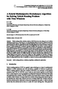
3. The Proposed Algorithm BEG-NSGA-II 3.1. Framework. In this paper, a two-stage optimization mechanism is used to solve the proposed VRPSPD with strict constraints. In the first stage, we use an improved bee evolutionary genetic algorithm to optimize the initial population. The optimization efficiency of the first stage is improved by optimizing the selection operators, selecting the different crossover operators according to the similarity of individuals’ parent chromosomes, and selecting the different mutation operators according to the performance of individual’s parent chromosome. In the second stage, an improved NSGA-II is used to optimize the proposed VRPSPD model. Based on the improved crossover and mutation operators, we construct the methods of deleting duplicate individuals, introducing new individuals, and using elite population instead of the parent population to improve the population diversity. To deal with the strict constraints, we introduce an external auxiliary population. During the optimizing process, if the constraint violation degree of the infeasible solutions is smaller than a given value, these infeasible solutions are copied to the external auxiliary population and used to evolve in the next generation. By using this external auxiliary population, the infeasible solutions gradually evolve to the boundary of feasible solutions, and the convergence speed is accelerated. The framework of the proposed algorithm is shown in Figure 2. More details of steps are described as follows. The first stage includes the following. Step 1. Randomly generate N different chromosomes to generate the initial population, and set t = 1, where N is the number of chromosomes and t is the current generation. Step 2. Calculate the constraint violation value of each chromosome with (17). If the number of individuals that meets the constraint conditions is greater than the specified value or t > T (T is the maximal iteration time in the first stage), jump over the first phase; otherwise go to step 3.
5 𝐼
𝐶𝑜𝑛𝑠𝑡 (𝑝) = ∑ max [0, 𝐷𝑟𝑖𝑓𝑡𝑝𝑖 − 𝐶𝑎𝑝𝑖 ] 𝑖=1
(17)
(𝑖 = 1, 2, . . . , 𝐼)
where Drift pi denotes the ith constraint condition value of chromosome P after decoding; Capi denotes the upper bound of the ith constraint condition. Step 3. Calculate each chromosome’s fitness based on the degree of constraint violation using (18); then select the best fitness individual as the queen; if t > 1, compare the fitness value of the queen with the parent queen, and select the better one as the new queen; if the number of feasible solutions is more than one, use nondominated sorting and congestion degree computing to deal with the feasible solutions to ensure that the queen selected from the parent population is the best one, then compare it with the parent queen, and select the better one as the new queen. 𝑓𝑖𝑡𝑛𝑒𝑠𝑠 (𝑝) =
1 (𝐶𝑜𝑛𝑠𝑡 (𝑝) + 1)
(18)
Step 4. Select 𝛾 individuals from the population using roulette wheel method. The number of 𝛾 is calculated by (19), where round [ ] means the operation of round; for example, round [2.3] equals 2. 𝛾 = round [
𝑡 𝑁 × ] 𝑇 2
(19)
Step 5. Randomly generate 𝛽 individuals different from each other, and combine them with the individuals generated from step 4. The number of 𝛽 is calculated by 𝛽=
𝑁 −𝛾 2
(20)
Step 6. The new queen takes crossover and mutation with other individuals generated from step 5 to produce the offspring population. Step 7. Delete the redundant repeating individuals and randomly generate M individuals different from each other into the population, where M equals the number of redundant repeating individuals that were deleted. Step 8. Return to step 2, and set t = t + 1. The second stage includes the following. Step 9. Take fast nondominated sorting and crowding degree calculation on population. Step 10. Carry out the following three kinds of operation for the population generated by step 9: select the top S (S=0.3N) individuals as the elite population; copy the individuals whose constraint violation values are less than a given value to the external auxiliary population 𝑆∗ ; use a binary tournament selection method to select crossover individuals and they were taken crossover according to the corresponding selected crossover methods to generate offspring.
6
Mathematical Problems in Engineering
Initial Randomly generated M individuals
Randomly generate N individuals that differ from each other
Y
Population number specified value or T>specified number of iterations
Select individuals by roulette wheel method
Scheduling and calculating fitness based on constraint violation degree
N
Y
If the number of feasible solutions is greater than 1, use non-dominated sorting and crowding degree calculating to deal with the feasible solutions; otherwise, the individual with largest fitness is the queen
Output result
t=t+1
Fast non-dominated sorting and crowding degree calculating, fitness assignment
Queen bee
Parent queen
Crossover and mutation
Transition population t=t+1
Y
N
t > max iteration number
Randomly generated individuals different from each other
Second stage
Select the best one as the new queen
Offspring population
t=1 Calculate the degree of violation of each chromosome
First stage
Delete duplicate individuals
Select crossover individuals by binary tournament selection
N
External auxiliary population M?N S∗
Offspring population
S (i,j) >
Y
Single-point crossover
Two-point crossover
Offspring rank=1 Elite population S
Select the best N individuals Fast non-dominated sorting and Crowding degree calculating
N
Y Transition population
TBM or Reverse mutation
Conventional mutation Offspring population
United population
N Y Population number GEN, output the result; otherwise, t = t + 1, and return step 10.
Step 1. A random parameter k that meets the inequality 0 𝜀,
Two-point crossover
(22)
(23)
The procedure of single-point crossover is described as follows (P1 and P2 are used to denote two parents; O1 and O2 are used to denote two offspring).
Step 3. The elements in P2 but not in O1 are duplicated to the remaining empty positions in O1 from left to right. Step 4. The elements in P1 but not in O2 are duplicated to the remaining empty positions in O2 from left to right. The procedure of two-point crossover is described as follows (P1 and P2 are used to denote two parents; O1 and O2 are used to denote two offspring). Step 1. Two random parameters k1 and k2 that meet the inequality 0 < k1 < k2 < L as well as k1 ≠ k2 are generated to determine the positions of crossover. Step 2. The elements from k1 to k2 in P1 are appended to the leftmost positions of O1 ; and the elements from k1 to k2 in P2 are appended to the leftmost positions of O2 . Step 3. The elements in P2 but not in O1 are duplicated to the remaining empty positions in O1 from left to right. Step 4. The elements in P1 but not in O2 are duplicated to the remaining empty positions in O2 from left to right. The examples of singe-point crossover and two-point crossover are, respectively, shown in Figures 3 and 4. 3.4. Mutation Operators. In this paper, we have adopted three different mutation operators for the purpose of expending the solution space as well as maintaining the good solutions, which are conventional mutation operator, reverse mutation operator, and TBM operator. The examples of these mutation operators are shown in Figures 5, 6, and 7. At this stage, every offspring inherits the excellent traits of the queen for it is generated by the mutation of individuals and queen. So we
8
Mathematical Problems in Engineering P1
2
1
9
10
0
3
4
6
0
5
7
8
O1
10
0
3
4
6
2
7
9
0
5
1
8
P2
2
7
9
10
0
3
4
6
0
5
1
8
O2
10
0
3
4
6
2
1
9
0
5
7
8
P1
2
1
9
10
0
3
4
6
0
5
7
8
Figure 4: Two-point crossover. P1
2
1
9
10
0
3
4
6
0
5
7
8
O1
2
1
9
4
0
3
10
6
0
5
7
8
Figure 5: Conventional mutation.
randomly chose a mutation operator with Pm probability at this stage. At the second stage, if the rank of offspring equals 1, we select the conventional mutation; otherwise we randomly select reverse or TBM mutation. The main procedure of conventional mutation operator is described as follows (P1 and O1 are used to denote a parent and offspring, respectively). Step 1. Randomly select two positions in P1 . Step 2. Swap the elements in the selected positions to generate O1 . The main procedure of reverse mutation operator is described as follows (P1 and O1 are used to denote a parent and offspring, respectively). Step 1. Randomly select two positions in P1 . Step 2. Reverse the numbers between the two selected positions to generate O1 . The main procedure of TBM operator is described as follows (P1 and O1 are used to denote a parent and offspring, respectively). Step 1. A random parameter m (m