DA3D: FAST AND DATA ADAPTIVE DUAL DOMAIN DENOISING. N. Pierazzo*, M.E. ..... For DA3D a Python implementation was used. Fig. 2: Test images used ...
DA3D: FAST AND DATA ADAPTIVE DUAL DOMAIN DENOISING N. Pierazzo? , M.E. Rais?† , J.M. Morel? , and G. Facciolo?‡ ´ CMLA, Ecole Normale Sup´erieure de Cachan, France † Dpt. Matem`atiques i Inform`atica, UIB, Spain ‡ ´ IMAGINE/LIGM, Ecole Nationale des Ponts et Chauss´ees, France ?
ABSTRACT This paper presents DA3D (Data Adaptive Dual Domain Denoising), a “last step denoising” method that takes as input a noisy image and as a guide the result of any state-of-the-art denoising algorithm. The method performs frequency domain shrinkage on shape and data-adaptive patches. Unlike other dual denoising methods, DA3D doesn’t process all the image samples, which allows it to use large patches (64 × 64 pixels). The shape and data-adaptive patches are dynamically selected, effectively concentrating the computations on areas with more details, thus accelerating the process considerably. DA3D also reduces the staircasing artifacts sometimes present in smooth parts of the guide images.The effectiveness of DA3D is confirmed by extensive experimentation. DA3D improves the result of almost all state-of-the-art methods, and this improvement requires little additional computation time. Index Terms— Image denoising, Patch-Based methods, Fourier shrinkage, Dual Denoising, Data Adaptive 1. INTRODUCTION Image denoising is one of the fundamental image restoration challenges [1]. It consists in estimating an unknown noiseless image y from a noisy observation x. We consider the classic image degradation model y = x + n, (1) where the observation x is contaminated by an additive white Gaussian noise n of variance σ 2 . All denoising methods assume some underlying image regularity. Depending on this assumption they can be divided, among others, into transform-domain and spatial-domain methods. Transform domain methods work by shrinking (or thresholding) the coefficients of some transform domain [2, 3, 4]. The Wiener filter [5] is one of the first such methods operating on the Fourier transform. Donoho et al. [6] extended it to the wavelet domain. Space-domain methods traditionally use a local notion of regularity with edge-preserving algorithms such as total variation [7], anisotropic diffusion [8], or the bilateral filter [9]. Nowadays however spatial-domain methods achieve remarkable results by exploiting the self-similarities of the image [10]. These patch-based methods are non-local as they denoise by averaging similar patches in the image. Patch-based denoising has developed into Aknowledgements: work partly founded by Centre National d’Etudes Spatiales (CNES, MISS Project), European Research Council (advanced grant Twelve Labours), Office of Naval research (ONR grant N00014-14-10023), DGA St´er´eo project, ANR-DGA (project ANR-12-ASTR-0035), FUI (project Plein Phare) and Institut Universitaire de France.
attempts to model the patch space of an image, or of a set of images. These techniques model the patch as sparse representations on dictionaries [11, 12, 13, 14, 15], using Gaussian Scale Mixtures models [16, 17], or with non-parametric approaches by sampling from a huge database of patches [18, 19, 20, 21]. Current state-of-the-art denoising methods such as BM3D [22] and NL-Bayes [23] take advantage of both space- and transformdomain approaches. They group similar image patches and jointly denoise them by collaborative filtering on a transformed domain. In addition, they proceed by applying two slightly different denoising stages, the second stage using the output of the first one as its guide. Some recently proposed methods use the result of a different algorithm as their guide for a new denoising step. Combining for instance, nonlocal principles with spectral decomposition [24], or BM3D with neural networks [25]. This allows one to mix different denoising principles, thus yielding high quality results [24, 25]. DDID [26] is an iterative algorithm that uses a guide image (from a previous iteration) to determine spatially uniform regions to which Fourier shrinkage could be applied without introducing ringing artifacts. Several methods [27, 28, 29] use a single step of DDID with a guide image produced by a different algorithm. This yields much better results than the original DDID. The reason for their success is the use of large (31 × 31) and shape-adaptive patches. Indeed, the Fourier shrinkage works better on large stationary blocks. Unfortunately, DDID has a prohibitive computational cost, as it paradoxically denoises a large patch to recover a single pixel. Moreover, contrary to other methods, aggregation of these patches doesn’t improve the results since it introduces blur. We show in this paper that these two problems can be solved by introducing a new patch selection, accompanied by a weighted aggregation strategy. Contribution. This paper presents DA3D (Data Adaptive Dual Domain Denoising), a new “last step” denoising method that performs frequency domain shrinkage on shape-adaptive and dataadaptive patches. DA3D consistently improves the results of stateof-the-art methods such as BM3D or NL-Bayes with little additional computation time. Similarly to DDID [26], DA3D uses a guide image to extract the shape-adaptive patches. But unlike it, DA3D processes only a fraction of the patches, which are aggregated instead of just taking their central pixel. The patches are dynamically selected, saving computations on uniform areas of the image to use them on areas with more details. This accelerates considerably the process, allowing to use even larger (64 × 64) patches, which in turn yields improved results. Some shape adaptive methods [30, 31] collectively denoise groups of similar small patches (8 × 8 blocks for BM3D-SAPCA [30]). DA3D does not consider groups, instead it uses much larger patches to extract more information from the underlying structure.
20.17 dB
37.00 dB
37.17 dB
37.99 dB
1.76%
38.07 dB
1.52%
20.17 dB
26.03 dB
26.05 dB
26.20 dB
16.9%
26.21 dB
16.5%
(a) Noisy
(b) Guide: NL-Bayes
(c) NL-Bayes + DDID step
(d) NL-Bayes + Sparse DDID
(e) Sparse DDID samples
(f) NL-Bayes + DA3D
(g) DA3D samples
Fig. 1: Results of applying different post-processing steps on the same image (with noise σ = 25). The guide was produced with Non-Local Bayes. Figs. (e) and (g) show the centers of the blocks used for denoising (d) and (f) respectively (with τ = 2). Image (c) was generated with 31 × 31 blocks, while for (d) and (f) 64 × 64 blocks were used. Notice in (d) and (f) the difference on che cheek and the forehead of the girl. Our second contribution in DA3D further improves the quality of the results by adapting the processing to the underlying data. The apparition of the staircasing is well known for non-local methods [32]. To mitigate the influence of such artifacts present in the guide image, we use a first order non-linear local kernel regression [33, 34] to estimate, for each patch, an affine approximation coherent with the data within the patch. The denoising is then performed with respect to this approximation. This data-adaptive approach is another innovation enabled by the use of large patches, and it noticeably improves the quality of the results on smooth regions of the image. Section 2 recalls the DDID postprocess. Sections 3 and 4 present the DA3D algorithm, first describing the proposed sparse aggregation, then the data-adaptive patches. The performance of DA3D is extensively validated in the experiments of section 5. 2. DUAL DOMAIN IMAGE DENOISING STEP A DDID step is a single iteration of the DDID algorithm [26], but it can also be used as a last denoising step for other methods [29, 27]. This section, along with the pseudocode in Table 1, summarizes it. To denoise a pixel p from the noisy image y the DDID step extracts a 31 × 31 pixel block around it (denoted y) and the corresponding block g from the guide image g. The blocks are processed to eliminate discontinuities that may cause artifacts in the subsequent frequency-domain denoising. To that end, the weight function k is derived from g. The weights identify the pixels of the block belonging to the same object as the center p. This weight function has the form of the bilateral filter [35, 9] � � � � |g(q) − g(p)|2 |q − p|2 exp − . (2) k(q) = exp − γr σ 2 2σs2 The first term identifies the pixels belonging to the same structure as p, by selecting the ones with a similar color in the guide, while the second term removes the periodization discontinuities associated with the Fourier transform. The parameters σs and γr are specific of the algorithm, and σ is the standard deviation of the noise. The weights k are then used to modify y and g in order to remove their discontinuities yielding ym and gm (see lines 13-14 of Table 1). In this way the “relevant” part of the blocks (similar to the central pixel) is retained by k, and its average value is assigned to the rest. The modified block ym is denoised by shrinkage of its Fourier coefficients using gm as an oracle (lines 15-18 of Table 1). Since
discontinuities have been removed from the blocks, filtering in the Fourier domain doesn’t introduce ringing, which is a major advance made by DDID in transform thresholding methods. The value of γf is a parameter of the algorithm. This shrinkage assumes that the image y contains additive white Gaussian noise. Finally, the denoised value of the central pixel is recovered by reversing the Fourier transform. This process is repeated for every pixel of the image. For more details about DDID refer to [26, 29]. For color images, k is computed by using the Euclidean distance, while the shrinkage is done independently on each channel of the YUV color space. An example of the result is shown in Fig. 1c. 3. SPARSE DDID STEP The DDID step explained in section 2 is slow because it has to process a block for every pixel. In fact, each pixel is denoised several times, but the result is discarded every time that it is not in the center of the current block. Since that the denoising remains valid for all pixels in the “relevant” part of the block, we propose to aggregate the processed blocks to form the final result. As a result, not every block needs to be processed, thus accelerating the algorithm considerably. Note that since the processing is done with the modified block, line 13 of Table 1 must be reverted to obtain the denoised block (line 20). In our selection-aggregation process, the image is treated by color-coherent blocks and the results are aggregated with weights deduced from the guide image. This weighted average can also be seen as the interpolation of the denoised image from a subset of processed blocks [36, 37, 38]. We found that the best aggregation weights are the squares of the weights (2). We now describe the greedy approach used for selecting the image blocks to be processed. At each iteration a weight map w with the sum of the aggregation weights is updated. This weight map permits to identify the pixel in the image with the lowest aggregation weight, which will be selected as the center of the next block to process (line 5 of Table 1). This process iterates until the total weight for each pixel becomes larger than a threshold τ . The weight function k is always equal to 1 in the center, so the algorithm always terminates. The procedure is detailed in Table 1. This variant is faster to execute than a single DDID step, since only a small number of blocks are actually processed. This allows bigger patches to be used, that in turn gives better results in terms of denoising quality. Experimentally, good results are achieved with patches as large
DDID Sparse DA3D • • • •
• • • • • •
• • • • • •
- - • • •
• •
• • • • •
• • • •
• • • •
• • • •
• • •
Input: y (noisy image), g (guide) Output: denoised image 1 w←0 2 out ← 0 3 for all pixels p ∈ y do 4 while min(w) < τ do 5 p ← arg min(w) 6 y ← E XTRACT PATCH(y, p) 7 g ← E XTRACT PATCH(g, p) // regression weight, eq. 4 8 Kreg ← C OMPUTE K REG(g) // regression plane, P eq. 3 9 P ← arg minP [y(q) − P (q)]2 · Kreg (q) 10 y ← y − P // subtract plane from the block 11 g ← g − P // and from guide 12 k ← C OMPUTE K(g) � // eq. 2 � P k(l)y(l) P 13 ym ← k · y + (1 − k) � P k(l) � k(l)g(l) P 14 gm ← k · g + (1 − k) k(l) 15 Y ← DFT(ym ) 16 G ← DFT(g P m) 17 σf2 ← σ 2 k(q)2 // shrinkage 1 � � if f = 0 2 18 K← γf σf exp − |G(f )|2 otherwise
• • • 19 •
• • -
• • • -
20
• -
• • •
• • •
24 25 26 27
21 22 23
xm ← IDFT(K · Y ) // revert �i h line 13 �P k(l)y(l) P /k x ← xm − (1 − k) k(l) x ← x + P // add plane back to the block aggw ← k · k // aggregation weight out(p) ← E XTRACT C ENTRAL P IXEL(xm ) // accumulate patch in the correct position w ← A DD PATCH AT(p, w, aggw) out ← A DD PATCH AT(p, out, aggw · x) return out return out/w
Table 1: Pseudo-code for DDID step, Sparse DDID and DA3D. The lines used only in the DDID step are highlighted in blue. Bullets show the operations of each algorithm. Variables in bold denote whole images, while italics denote single blocks. Multiplication and division are pixel-wise.
Method BM3D SAPCA [30] BM3D [22]
DDID [26]
G-NLM [24]
LSSC [13]
σ =5 38.43 38.39 -0.04 38.24 38.24 +0.00 37.95 37.90 -0.04 37.91 35.67 +0.60 38.29 38.34 +0.05
MLP + BM3D [25] NLB [23]
NLDD [29]
NLM [10]
PID [28]
SAIST [15] Average
38.19 38.20 +0.02 38.12 38.09 -0.04 37.31 37.49 +0.18 37.97 37.90 -0.07 38.31 38.31 -0.01 +0.06
σ = 10 34.94 34.95 +0.01 34.70 34.78 +0.08 34.55 34.52 -0.03 34.29 33.97 +0.43 34.75 34.88 +0.13 34.63 34.78 +0.15 34.62 34.72 +0.10 34.62 34.60 -0.02 33.58 33.98 +0.40 34.56 34.48 -0.08 34.78 34.82 +0.04 +0.11
σ = 25 30.58 30.67 +0.10 30.37 30.54 +0.16 30.34 30.39 +0.05 29.90 29.77 +0.58 30.35 30.61 +0.27 30.44 30.61 +0.17 30.13 30.38 +0.25 30.30 30.29 -0.01 28.97 29.66 +0.69 30.38 30.28 -0.10 30.39 30.53 +0.14 +0.22
σ = 40 28.27 28.41 +0.14 27.99 28.23 +0.24 28.05 28.16 +0.11 27.64 27.49 +0.63 28.07 28.32 +0.25
σ = 80 24.69 25.09 +0.39 24.94 25.03 +0.09 24.68 24.84 +0.16 24.46 24.10 +0.65 24.78 24.97 +0.19
27.86 28.14 +0.28 28.11 28.09 -0.02 26.50 27.45 +0.95 28.18 28.08 -0.11 28.16 28.27 +0.11 +0.27
24.45 24.78 +0.33 24.83 24.77 -0.05 22.72 24.17 +1.44 24.99 24.81 -0.18 25.00 25.07 +0.07 +0.31
Table 2: Average PSNR comparison between state-of-the-art methods on grayscale images. The first line of each row shows the average PSNR. The second line shows the average PSNR of DA3D using the corresponding algorithm to generate the guide. The third line shows the average improvement due to DA3D. The best result for each noise level is shown in bold, and the ones within a range of 0.2 dB are shown in gray. MLP+BM3D only works with some specific levels of noise, the other levels are left blank.
as 64 × 64, which is to be contrasted to patch based methods using mostly 8 × 8 patches. An example of the result is shown in Fig. 1d. The total number of processed blocks depends on the image complexity. The centers of the effectively processed blocks are shown in Fig. 1e. They concentrate on edges and details.
method can be extended to “normalize” each patch by subtracting an estimation of the gradient around the patch center. In practice, this means estimating an affine model of the block, as proposed in [33], which can be computed using a weighted least squares regression X min [y(q) − P (q)]2 · Kreg (q), (3)
4. DATA ADAPTIVE DUAL DOMAIN DENOISING
where the sum is computed over the domain of y and Kreg is a bilateral weight function � � |q − p|2 |g(q) − g(p)|2 − , (4) Kreg (q) = exp − 2 γrr σ 2 2σsr
P
We now address a main drawback of the weight function (2), used for the bilateral filter and for many bilateral-inspired filters, including patch based methods. This weight function selects pixels of the block with a similar value. As a result, Sparse DDID works by processing parts of the image that are piecewise constant, considering the image as composed by many “flat” layers. This model is not well adapted for images that contain gradients or shadings, as the same smooth region may be split in many thin regions. The previous
which selects the parts of the block that gets approximated by P . To ensure that the central pixel gets denoised, the constraint P (p) = g(p) is also added. Since the weights Kreg should capture the overall shape of the block, they are computed using a larger range parameter than the bilateral weight function in (2). It is worth noting
Image Size 256×256 512×512
G-NLM 357 s 3359 s
SAPCA 639 s 2490 s
NLB 0.48 s 0.80 s
PID 188 s 725 s
BM3D 1.26 s 4.94 s
SAIST 37.8 s 140 s
MLP 16.5 s 60.7 s
EPLL 71.7 s 272 s
NLDD 1.97 s 7.25 s
DDID 5.26 s 20.4 s
BM3D+DA3D 2.92 s 9.62 s
Table 3: Average running time depending on image size between grayscale denoising methods. The experiments were performed on a 8-core 2.67GHz Xeon CPU. Every algorithm was tested using its official implementation. For DA3D a Python implementation was used.
32.764 dB
(a) Original Fig. 2: Test images used in the experiments. No parameter learning or fitting was performed on this database. that although Kreg uses the guide to select the parts of the block in which to perform the estimation, the regression is performed directly on the noisy data y, thus allowing to correct any staircasing effect already present in the guide. The parameters σsr and γrr are specific of the algorithm. The case of color images is identical, since (3) is separable and can be computed independently on every channel. Once estimated, the local plane P is subtracted from the patch, effectively removing shades and gradients. Then the standard DDID step is used to denoise the block and at the end the plane is added back. The whole procedure is detailed in Table 1 (lines 8-11, 21). An example of the result is shown in Fig. 1f. Observe that the result present less staircasing effect and is better in terms of PSNR. In addition, less blocks are treated to denoise the gradients (Fig. 1g). 5. EXPERIMENTS Our implementation of the DA3D algorithm (available in the support website [39]) has been tested against the set of images shown in Fig. 2. For γr and γf , the parameters of DDID [26] were kept (γr = 0.7, γf = 0.8), but since DA3D does not need to process all patches, the size of the patches themselves was chosen as 64 × 64, with σs = 14. The parameters τ = 2, σsr = 20 and γrr = 7 were chosen experimentally on images outside the test database. The DA3D method was applied to the results of several stateof-the-art algorithms. Each method was tested with noises of σ = 5, 10, 25, 40, 80. The results are summarized in Table 2. DA3D improves the PSNR of every algorithm except NLDD and PID (which is to be expected, since they are based on a similar shrinkage strategy). This improvement is more marked with higher noises, which makes sense since the parameters of DDID were optimized for medium to high noise. It is worth mentioning that DA3D is even able to improve over BM3D-SAPCA, which is considered the best denoising algorithm up to date for grayscale images. Similar results are obtained using SSIM [40] as metric. In general BM3D+DA3D (DA3D using BM3D as guide) offers one of the best performances with a reasonable computational cost. As an example the results of the best two performing methods for the image “Montage” are shown in Fig. 3, along with the result of BM3D+DA3D. The latter outperforms the other algorithms in terms of PSNR and image quality. Despite having a high PSNR value, the result of the other two algorithms present artifacts close to the edges and some staircasing (BM3D-SAPCA in particular). The results for color images are similar to the grayscale case.
(b) BM3D-SAPCA
32.724 dB
(c) PID
32.998 dB
(d) BM3D+DA3D
Fig. 3: Denoising results for Montage, σ = 25. A zoom-in is advised to see the staircasing effects in (b) and (c) and their removal in (d).
39.452 dB
(a) Original
(b) BM3D
38.999 dB
(c) NL-Bayes
40.303 dB
(d) BM3D+DA3D
Fig. 4: Denoising results for Dice, σ = 25. As before, NLDD and PID are not improved (or just marginally improved) by DA3D. The detailed tables with PSNR and SSIM are available in the support website [39]. Fig. 4 shows the two best denoising results for the image “Dice”, along with the result of BM3D+DA3D. Most of the artifacts generated by BM3D disappear with the post-processing, and at the same time the edges becomes sharper and the gradients smoother. Running time. The time needed to run the analyzed algorithms is summarized in Table 3. Using DA3D as a post-processing method demands little additional time, while the gain is substantial (in PSNR and in visual quality). Therefore, while BM3D+DA3D is comparable to BM3D-SAPCA in terms of performance, its computation is more than 200 time faster.
6. CONCLUSIONS AND FUTURE WORK This paper presented DA3D, a fast Data Adaptive Dual Domain Denoising algorithm for “last step” processing. It performs frequency domain shrinkage on shape and data-adaptive patches. The key innovations of this method are a sparse processing that allows bigger blocks to be used and a plane regression that greatly improves the results on gradients and smooth parts. The experiments show that DA3D can improve the results of most denoising algorithms with reasonable computational cost, achieving a performance superior to the state-of-the-art. Future work will include optimizing the parameters of the algorithm, especially for low levels of noise, and adapting the shrinkage function to the algorithm used as guide.
7. REFERENCES [1] M. C. Motwani, M. C. Gadiya, R. C. Motwani, and F. C. Harris Jr., “Survey of image denoising techniques,” GSPX, 2004.
[21] I. Mosseri, M. Zontak, and M. Irani, “Combining the power of internal and external denoising,” IEEE ICCP, pp. 1–9, April 2013.
[2] J. L. Starck, E. J. Cand`es, and D. L. Donoho, “The curvelet transform for image denoising,” IEEE TIP, vol. 11, no. 6, 2002.
[22] K. Dabov, A. Foi, V. Katkovnik, and K. Egiazarian, “Image denoising by sparse 3d transform-domain collaborative filtering,” IEEE TIP, vol. 16, no. 82, 2007.
[3] H. Q. Li, S. Q. Wang, and C. Z. Deng, “New image denoising method based wavelet and curvelet transform,” WASE ICIE, vol. 1, 2009.
[23] M. Lebrun, A. Buades, and J. M. Morel, “Implementation of the ”non-local bayes” (NL-bayes) image denoising algorithm,” Image Processing On Line, 2013.
[4] D. Gnanadurai and V. Sadasivam, “Image denoising using double density wavelet transform based adaptive thresholding technique,” IJWMIP, vol. 03, no. 01, 2005.
[24] H. Talebi and P. Milanfar, “Global image denoising,” IEEE TIP, vol. 23, no. 2, pp. 755–768, Feb 2014.
[5] N. Wiener, Extrapolation, Interpolation, and Smoothing of Stationary Time Series, The MIT Press, 1964. [6] D. L. Donoho and J. M. Johnstone, “Ideal spatial adaptation by wavelet shrinkage,” Biometrika, 1994. [7] L. I. Rudin, S. Osher, and E. Fatemi, “Nonlinear total variation based noise removal algorithms,” Phys. D, vol. 60, 1992. [8] P. Perona and J. Malik, “Scale-space and edge detection using anisotropic diffusion,” IEEE TPAMI, vol. 12, no. 7, pp. 629– 639, Jul 1990. [9] C. Tomasi and R. Manduchi, “Bilateral filtering for gray and color images,” IEEE ICCV, 1998. [10] A. Buades, B. Coll, and J. M. Morel, “A review of image denoising algorithms, with a new one,” SIAM Mult. Model. Simul., vol. 4, no. 2, 2006. [11] M. Elad and M. Aharon, “Image denoising via sparse and redundant representations over learned dictionaries,” IEEE TIP, vol. 15, no. 12, 2006. [12] J. Mairal, G. Sapiro, and M. Elad, “Learning multiscale sparse representations for image and video restoration,” SIAM Mult. Model. Simul., vol. 7, no. 1, 2008. [13] J. Mairal, F. Bach, J. Ponce, G. Sapiro, and A. Zisserman, “Non-local sparse models for image restoration,” IEEE ICCV, pp. 2272–2279, Sept 2009. [14] G. Yu, G. Sapiro, and S. Mallat, “Image modeling and enhancement via structured sparse model selection,” IEEE ICIP, 2010. [15] W. Dong, G. Shi, and X. Li, “Nonlocal image restoration with bilateral variance estimation: A low-rank approach,” IEEE TIP, vol. 22, no. 2, pp. 700–711, 2013. [16] D. Zoran and Y. Weiss, “From learning models of natural image patches to whole image restoration,” IEEE ICCV, pp. 479– 486, Nov 2011. [17] J. Portilla, V. Strela, M. J. Wainwright, and E. P. Simoncelli, “Image denoising using scale mixtures of gaussians in the wavelet domain,” IEEE TIP, 2003. [18] A. Levin and B. Nadler, “Natural image denoising: Optimality and inherent bounds,” IEEE CVPR, 2011. [19] A. Levin, B. Nadler, F. Durand, and W. T. Freeman, “Patch complexity, finite pixel correlations and optimal denoising,” IEEE ECCV, pp. 73–86, 2012. [20] N. Pierazzo and M. Rais, “Boosting shotgun denoising by patch normalization,” IEEE ICIP, 2013.
[25] H. C. Burger, C. Schuler, and S. Harmeling, “Learning how to combine internal and external denoising methods,” in Pattern Recognition, vol. 8142 of Lecture Notes in Computer Science, pp. 121–130. Springer Berlin Heidelberg, 2013. [26] C. Knaus and M. Zwicker, “Dual-domain image denoising,” IEEE ICIP, 2013. [27] C. Knaus, Dual-domain image denoising, Ph.D. thesis, Diss. Univ. Bern, 2013, Bern, 2013. [28] C. Knaus and M. Zwicker, “Progressive image denoising,” IEEE TIP, vol. 23, no. 7, pp. 3114–3125, July 2014. [29] N. Pierazzo, M. Lebrun, M. Rais, J. M. Morel, and G. Facciolo, “Non-local dual image denoising,” IEEE ICIP, 2014. [30] K. Dabov, A. Foi, V. Katkovnik, and K. Egiazarian, “BM3D Image Denoising with Shape-Adaptive Principal Component Analysis,” SPARS, 2009. [31] C. A. Deledalle, V. Duval, and J. Salmon, “Non-local methods with Shape-Adaptive patches (NLM-SAP),” JMIV, vol. 43, no. 2, pp. 103–120, May 2012. [32] A. Buades, B. Coll, and J. M. Morel, “The staircasing effect in neighborhood filters and its solution,” IEEE TIP, vol. 15, no. 6, pp. 1499–1505, June 2006. [33] H. Takeda, S. Farsiu, and P. Milanfar, “Kernel regression for image processing and reconstruction,” IEEE TIP, vol. 16, no. 2, pp. 349–366, February 2007. [34] H. Takeda, S. Farsiu, and P. Milanfar, “Higher order bilateral filters and their properties,” Electronic Imaging, p. 64980S, 2007. [35] L. P. Yaroslavsky, “Local adaptive image restoration and enhancement with the use of DFT and DCT in a running window,” Proceedings of SPIE, 1996. [36] F. Durand and J. Dorsey, “Fast bilateral filtering for the display of high-dynamic-range images,” ACM SIGGRAPH, pp. 257– 266, 2002. [37] A. B. Adams, High-dimensional gaussian filtering for computational photography, Stanford University, 2011. [38] E. Gastal and M. M. Oliveira, “Adaptive manifolds for realtime high-dimensional filtering,” ACM Trans. Graph., vol. 31, no. 4, July 2012. [39] Authors, “DA3D support website and supplementary material,” http://dev.ipol.im/˜pierazzo/da3d, 2015. [40] Z. Wang, A. C. Bovik, H. R. Sheikh, and E. P. Simoncelli, “Image quality assessment: From error visibility to structural similarity,” IEEE TIP, vol. 13, no. 4, 2004.