Data-Driven Decision Tree Classification for ... - Semantic Scholar

Data-Driven Decision Tree Classification for Product Portfolio Design Optimization Conrad S. Tucker e-mail: [email protected]

Harrison M. Kim1 Assistant Professor Mem. ASME e-mail: [email protected] Department of Industrial and Enterprise Systems Engineering, University of Illinois at Urbana-Champaign, 104 S. Mathews Avenue, Urbana, IL 61801

1

The formulation of a product portfolio requires extensive knowledge about the product market space and also the technical limitations of a company’s engineering design and manufacturing processes. A design methodology is presented that significantly enhances the product portfolio design process by eliminating the need for an exhaustive search of all possible product concepts. This is achieved through a decision tree data mining technique that generates a set of product concepts that are subsequently validated in the engineering design using multilevel optimization techniques. The final optimal product portfolio evaluates products based on the following three criteria: (1) it must satisfy customer price and performance expectations (based on the predictive model) defined here as the feasibility criterion; (2) the feasible set of products/variants validated at the engineering level must generate positive profit that we define as the optimality criterion; (3) the optimal set of products/variants should be a manageable size as defined by the enterprise decision makers and should therefore not exceed the product portfolio limit. The strength of our work is to reveal the tremendous savings in time and resources that exist when decision tree data mining techniques are incorporated into the product portfolio design and selection process. Using data mining tree generation techniques, a customer data set of 40,000 responses with 576 unique attribute combinations (entire set of possible product concepts) is narrowed down to 46 product concepts and then validated through the multilevel engineering design response of feasible products. A cell phone example is presented and an optimal product portfolio solution is achieved that maximizes company profit, without violating customer product performance expectations. 关DOI: 10.1115/1.3243634兴

Introduction

The emergence of highly competitive markets in the global marketspace has forced companies to reevaluate strategies in ensuring sustainable business endeavors. Attempts to satisfy a wide array of customers quickly and efficiently have led to the concept of product customization, wherein enterprise decision makers strive to better cater to the needs of their customers through a wider array of products to choose from 关1兴. While this approach is beneficial to the consumer, such design and manufacturing decisions can lead to adverse effects from a manufacturing, distribution, and marketing cost standpoint. Companies continue to place a high premium on the methodologies needed to ensure that mass customization decisions lead to increased or, at the very least, consistent profit margins. Attempts to mitigate the added costs of mass customization are in part achieved through the product family paradigm 关2兴, wherein products that satisfy the individual product functionality requirements dictated by customer preference are designed around a shared and efficient product architecture. The term product architecture is frequently defined as the set of modules/components wherein product variants evolve 关3–6兴. Commonality among product variants can translate into lower manufacturing costs associated with highly differentiated products through economies of scale 关7,8兴. The challenges facing enterprise decision makers in the product portfolio development process are multifaceted and include identifying candidate product concepts that have the greatest probability of market success. Attempts to search every pos1

Corresponding author. Contributed by the Engineering Informatics Division of ASME for publication in the JOURNAL OF COMPUTING AND INFORMATION SCIENCE IN ENGINEERING. Manuscript received December 20, 2007; manuscript received February 16, 2009; published online November 2, 2009. Paper presented at the 2007 IDETC, Las Vegas, NV. Assoc. Editor: K. Law.

sible product concept may be impractical in real life design processes, especially when first to market may create tremendous competitive advantages in the market space. Our approach to product portfolio formulation takes large data sets of customer preference data and extracts meaningful product attribute information to help guide the actual product design and development process. The overall objective of maximizing company profit is realized when a feasible set of product variants is presented in the final solution process. The reduction in resources in this limited and highly efficient narrowing of product concepts will be demonstrated through a cell phone example, where an entire product concept generation space of 576 共exhaustive combination of product attributes兲 product concepts is narrowed to only 46 through a decision tree data mining approach. The generated product designs are then subsequently tested for engineering feasibility. This is formulated as a multilevel optimization problem, where the generated predictive product concepts are first translated into functional specifications and set as targets at the engineering level for design validation. A feasible product design is therefore defined as one in which all customer preferences are satisfied, without violating engineering design constraints. This paper is organized as follows. This section provides a brief motivation and background. Section 2 describes previous works closely related to the current research. Section 3 describes the methodology. The methodology is demonstrated in Sec. 4 through a cellular phone portfolio design example. Section 5 presents the results and discussion. Section 6 concludes the paper.

2

Related Work

2.1 Customer Knowledge Acquisition Approaches. There are several well established methods for translating customer requirements into tangible engineering design targets in the product development process. We will briefly review several well known

Journal of Computing and Information Science in Engineering Copyright © 2009 by ASME

DECEMBER 2009, Vol. 9 / 041004-1

Downloaded 04 Jun 2010 to 128.174.193.86. Redistribution subject to ASME license or copyright; see http://www.asme.org/terms/Terms_Use.cfm

approaches in Secs. 2.1.1–2.1.3, and in Sec. 2.1.4, we highlight the strengths of data mining as an alternative approach for acquiring customer product requirements. 2.1.1 Quality function deployment. The quality function deployment 共QFD兲 is a design and development methodology that attempts to acquire customer requirements 共CRs兲 otherwise known as the voice of the customer 共VOC兲 and translate them into functional engineering targets 关9兴. A conventional approach to customer requirement acquisition is through focus group interviews or conducting surveys of a sample of current or future customers 关10兴. Corresponding weights are assigned to each customer requirement based on an importance rating indicated by a customer 关11,12兴. A QFD matrix is often used to depict the interdependence between customer requirements and the engineering metrics 共EMs兲 and to aid in brainstorming and designing the optimal product to address customer needs. QFD driven product development methodologies suggest that QFD is well suited for out of the box solutions to customer needs due to the fact that engineering design features are evaluated based on their positive and negative contributions to solving the product design problem 关9兴. The design of the QFD matrix also makes it easier to benchmark a particular design solution against competing brands. 2.1.2 Conjoint analysis. Conjoint analysis 共CA兲 has been used successfully in marketing to determine how customers value combinations of different product attributes/features 关9兴. In this approach, a target customer group is identified for the study and presented with a set of attributes 共survey format or prop cards 关13兴兲, each with different levels 共attribute ranges兲关14兴. Part-worth utilities are estimated based on customer importance ranking of individual product attributes. The resulting utility function is used to evaluate customer preferences for different attribute combinations. Although conjoint analysis application areas can range from human psychology to advertising, attempts to directly incorporate it into engineering design optimization and product development have been investigated 关15–18兴. These conjoint analysis based product development methodologies highlight the ability of the approach to quantify specific product attribute levels in new product development. However, this approach is primarily survey driven and therefore as the attribute space becomes large, preserving the quality of the model becomes a challenge. 2.1.3 Discrete choice analysis. Discrete choice analysis 共DCA兲 is the modeling methodology of consumer choice behavior from a set of mutually exclusive collective exhaustive alternatives 关19兴. DCA incorporates probabilistic choice theory in determining which product a customer is most likely to choose based on expected utility 关20兴. In engineering design and development, modeling product demand can therefore be based on a customer utility function model that incorporates unknown parameter estimates and unobservable customer utility components 关21–23兴. Instances of discrete choice analysis include the probit model and logit models 共multinomial, mixed, nested, etc.兲 to name but a few. In product development, applications are focused on creating consumer choice models either through stated or revealed data 关23–26兴. Many of these studies reveal the strengths of DCA in quantifying the market share of different brands of products given a set of attributes. The DCA model presents enterprise decision makers and design engineers with relevant probability measures of choosing one product over another based on product characteristics. A challenge of using DCA that is reported in the literature is that of multicollinearity, where it becomes difficult to generate a DCA model due to the presence of highly correlated attributes. 2.1.4 Data mining and knowledge extraction in product development. A few fundamental differences between data mining techniques and those discussed in Secs. 2.1.1–2.1.3 are that unlike the QFD and CA techniques that are highly dependent on stated preference data acquired through close customer interaction, data mining applications can also deal with revealed preference data 041004-2 / Vol. 9, DECEMBER 2009

共real customer purchase behavior that is captured through purchase transactions 共in-store, online, etc.兲关26兴. The absence of the direct customer interaction constraints allows larger data sets to be analyzed through data mining techniques that, in turn, may more accurately reflect the individual preferences of a wider array of customers. In relation to attribute importance, both the QFD and CA extract attribute importance 共or relevance兲 by either requiring customers to rank individual product attributes or rank product concepts as a whole. This added requirement to rank product alternatives or attributes may also limit the size of the data set that can be analyzed or the speed and efficiency by which new products can be designed. In the predictive data mining technique presented in this work, customers are not required to rank product alternatives or attributes. Instead they are only required to select the combination of attributes and price that most closely meet their needs. Product attribute importance is therefore identified during the decision tree model generation by employing the gain ratio attribute evaluation metric discussed later in Sec. 3.1.3. Therefore no prior attribute ranking is assumed or required. The incorporation of data mining techniques in product portfolio development is emerging as a well-founded approach to extracting and analyzing relevant customer information. Kusiak and Smith highlighted several key areas in industrial and manufacturing design processes, where data mining techniques could potentially have great benefits 关27兴. In the context of product portfolio development, the application of data mining clustering techniques in the design of modular products has also been investigated. Moon et al. used data mining to represent the functional requirements of customers and used fuzzy clustering techniques to determine the module composition of a product architecture 关1兴. Nanda et al. proposed a product family ontology development methodology 共PFODM兲 that utilizes a formal concept analysis approach in the design of product families 关28兴. This approach incorporates existing knowledge of the product family in generating a hierarchical conceptual clustering of design components. Data mining predictive techniques are investigated by Tucker and Kim to extract knowledge from large customer product preference data sets. This approach incorporates customer input at the early stages of the design process by directly integrating customer predictive preferences with engineering design through a data mining Naive Bayes predictive technique 关29兴. The decision tree generation approach that we adopt in this work presents an enterprise decision maker with product concepts that are determined to be the best indicators for market success 关20兴. This prediction is based on the C4.5 machine learning algorithm that predicts a certain class variable by selecting a particular customer attribute combination that are the best predictors 共based on the C4.5 algorithm discussed in Sec. 3.1.3 of this particular class variable兲 of a particular class value 关30,31兴. The speed and efficiency of the C4.5 algorithm, together with the ease of interpreting the decision tree structure make this data mining approach suitable for the product design scenario that we present in this work. 2.2 The Concept of Novel Previously Unknown Customer Information. The term product concept that we define in this work relates to the notion of novel previously unknown customer information that data mining is well known for 关32–34兴. To illustrate this concept, we present a simple test data set represented in Table 1. The data set contains six customer attributes 共columns 1–6兲 with one predictor variable 共Class variable in column 7兲. Based on the attribute values in Table 1 of Feature, Priority, Type, Connectivity, Battery Life, and Display, there are a total of 3 · 2 · 2 · 3 · 3 · 2 = 216 possible unique combinations 共although only 10 out of the 216 combinations exist in the sample data in Table 1兲. Two fundamental questions arise from our observation. •

How can we determine novel attribute combinations without performing additional data acquisition procedures 共customer surveys, focus groups, etc.兲? Transactions of the ASME


Table 1 Example data set of customer attributes

•

Feature

Priority

Type

Connectivity

Battery life

Display

MaxPrice

MP3 MP3 MP3 MP3 Camera Camera Games Games Games Games

Cost Weight Weight Cost Weight Weight Cost Cost Weight Cost

Flip Flip Flip Shell Shell Flip Flip Shell Flip Flip

Bluetooth Wifi Bluetooth Infrared Wifi Wifi Bluetooth Wifi Infrared Bluetooth

5 3 3 5 3 3 5 7 5 3

Screen size Screen size Resolution Screen size Screen size Resolution Resolution Resolution Screen size Screen size

200 160 160 80 120 120 200 200 160 160

How efficiently can we extract these new attribute combinations?

The term novel in our work relates to information that is not readily observable or not explicitly defined within the data set but can be quantified through the proposed decision tree induction technique. The following product design question aims to illustrate how novel information can be extracted from a raw data set. •

Given a specific attribute combination not existing within the data set 共for example, referring to Table 1 in the paper, we observe that the combination of 兵Games, Weight, Flip, Bluetooth, 5 h battery, ScreenSize其 does not exist within the data set兲.

1. What price category 共MaxPrice兲 would the above attribute combination fall under? 2. Are all of these attributes needed to predict the price category? That is, if we include only a subset of the attribute space 兵Games, Weight, and Flip其 instead of the entire attribute space 兵Games, Weight, Flip, Bluetooth, 5 h battery, and ScreenSize其, would it still result in the same price category 共MaxPrice兲 prediction? The case study example in Sec. 4.1.1 helps address these questions. For example, the decision tree structure in Fig. 2 reveals that for the Games phone, as long as the product also includes bluetooth connectivity and a 5 h battery life, we would result in a predicted price of $120. Therefore if design engineers were aiming to design the next generation of Games phones to a customer market segment willing to pay $120, then these product attributes would make up the primary product architecture. Another example of attribute knowledge discovery can be observed in Table 1. If we were to design a camera phone product, we see from rows 5 and 6 that both Camera phones, each with

slightly different attribute combinations yield a purchase price of $120. However, based on the C4.5 algorithm 共explained in Sec. 3.1.3兲, we observe that no additional attributes are needed to yield a Camera phone price of $120 共see the initial partitioning in Table 2兲, therefore from a product design perspective, no additional resources should be invested in improving additional design features that do not significantly influence the purchase decisions of a customer. This type of information is not readily observed in the raw data set and will enable design engineers to design the next generation of Games and Camera phones by including only the relevant attributes along with their predicted attribute levels. Such insights have the potential to save on manufacturing and materials costs, as well as on the time and efficiency of the product design process. The term product concepts used in this work therefore represents attribute combinations within the data set 共some of which may not appear in the raw data set兲 that are generated by the C4.5 predictive model 关31,35兴. Herein lies one of the fundamental strengths of data mining as opposed to the other customer data collection techniques presented in Sec. 2.1 in that inferences can be made on attribute combinations not readily available in the raw data set without additional customer interactions. The underlying structure of the C4.5 decision tree algorithm allows us to quantify such hidden patterns within the raw data set. We discuss the theoretical aspects of the C4.5 decision tree algorithm in Sec. 3.1.3 and demonstrate how the classification procedure employed by the algorithm has the potential of classifying novel, previously unknown attribute combinations 关31,36兴. Note: the data set of 40,000 customer responses used in the case study in Sec. 4 has the same attributes as those found in Table 1; however, since it is the complete data set, all of the attribute values are present in the data set. For example, the Feature at-

Table 2 Test data for decision tree generation Feature

Priority

Type

MP3 MP3 MP3 MP3

Cost Weight Weight Cost

Flip Flip Flip Shell

Camera Camera

Weight Weight

Games Games Games Games

Cost Cost Weight Cost

Connectivity

Battery life

Display

MaxPrice

Branch 1 Bluetooth Wifi Bluetooth Infrared

5 3 3 5

Screen size Screen size Resolution Screen size

200 160 160 80

Shell Flip

Branch 2 Wifi Wifi

3 3

Screen size Resolution

120 120

Flip Shell Flip Flip

Branch 3 Bluetooth Wifi Infrared Bluetooth

5 7 5 3

Resolution Resolution Screen size Screen size

200 200 160 160

Journal of Computing and Information Science in Engineering

DECEMBER 2009, Vol. 9 / 041004-3


Fig. 1 Overall flow of product portfolio optimization process.

tribute has 6 levels in the data set of 40,000, but since we used a sample in Table 1 for illustrative purposes, all 6 values of the Feature attribute do not show up.

3

Methodology

The entire product portfolio generation process is divided into two phases. Phase 1 is the customer knowledge discovery process, which entails customer data acquisition, processing, and data mining for feasible set generation. Phase 2 involves the product concept validation through multilevel optimization and finishes with a product portfolio selection. Figure 1 shows the overall flow of this process 共the general flow on the left and the detailed flow on the right of Fig. 1兲 starting with customer data acquisition and ending with enterprise portfolio selection. The details of the methodology are presented as follows.

3.1 Phase 1: Customer Knowledge Discovery. Knowledge discovery in databases 共KDDs兲 has become known as the nontrivial means of extracting information in large scale databases that were previously too complex for human analysis 关37兴. Data mining techniques utilize classification algorithms to extract meaningful previously unknown information from large data sets 关33兴. The concept of data mining can be applied to product portfolio formulation, wherein the exact product specifications and manufacturing quantity 共predicted demand information for each individual product concept兲 can be determined directly from data mining predictions. The process from data extraction to predictive model is as follows. 3.1.1 Data acquisition. The acquisition and storage of data are paramount in the product portfolio formulation process. We first begin by acquiring the raw data set to be used in the data mining

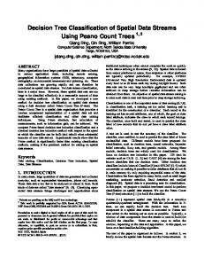
Fig. 2 C4.5 decision tree solution for 40,000 customer data set

041004-4 / Vol. 9, DECEMBER 2009

Transactions of the ASME


sequence. This data can be acquired in several ways. One approach is by conducting a realistic customer survey to capture what customers want and then translating these wants into meaningful engineering design targets 关38兴. Another approach would be for this data to already exist in a data warehouse, i.e., stored data from past customer purchasing behavior 共e.g., Structured Query Language server 共SQL兲兲关39兴. To increase the predictive capabilities of a classifier, it is often encouraged that the data set be large enough to accurately test the generated model with a portion of the data set. 3.1.2 Data preprocessing: data selection, cleaning, and transformation. The data preprocessing stage is where irrelevant or noisy data are identified and removed, and relevant data are extracted from the raw data 关39兴. There are many well established approaches that deal with missing attributes or ambiguous responses ranging from the most common attribute, event covering method, or ignoring the value altogether 关40–42兴. When dealing with electronic transactional data 共online and in-store兲, it is then possible to collect, clean, and store these data in a data warehouse. A data warehouse is a preprocessing stage that integrates all data into one source 共this includes raw data, historical data, summarized data, etc.兲关43兴. The accuracy of the data mining model will be highly dependent on the data selection and cleaning step, and it is therefore important that considerable time be allocated to preparing high quality data for the pattern discovery step that follows. There are many algorithms that exist in today’s data mining analysis tools that are now capable of incorporating this data selection and cleaning process directly with the overall knowledge discovery process 关44,45兴. The final data preprocessing step involves transforming the data into acceptable forms for the appropriate mining algorithm. Data transformations can include binning, normalizing, missing value imputation, etc. 关46兴. This can either be done manually by the user or automatically by the analysis tool 关45兴. 3.1.3 Pattern discovery. First a particular algorithm is selected and for the predictive analysis for our cell phone architecture design, we have opted to incorporate the C4.5 machine learning algorithm to generate a set of attribute combinations suitable for engineering design evaluation. Each unique attribute combination that predicts a class variable will be considered a candidate product concept. Typically, data mining techniques utilize 2/3 of the raw data to train the machine and the remaining 1/3 to test the model developed. The N-fold cross validation technique selects and compares several test models with one another and selects the appropriate model that best predicts the class variable 关45兴. The C4.5 machine learning algorithm for generating these product concepts is described more in detail below. 3.1.3.1 Product concept generation using C4.5 machine learning algorithm. Our approach to product concept generation adopts the C4.5 data mining tree generation technique first proposed by Quinlan 关30兴. The algorithm is based on the divide and conquer 关31,30兴 technique that decomposes a set of training cases T with class variables 兵C1 , C2 , . . . , CN其 until the partitioning yields a collection of cases that predicts a single class variable Ci. Each subsequent decomposition of the tree tests a single attribute that has outcomes 兵O1 , . . . , O P其 that are mutually exclusive to one another 关31兴. When applied to product portfolio optimization, the class variable can be thought of as the overall performance criteria 共determined by the enterprise decision maker兲 influencing product launch decisions. The class variable selected by the enterprise decision maker can range from a Price metric 共later to be demonstrated in our cell phone example兲 to a Weight or Dimensionality metric, etc. The manner in which attributes are selected during each stage of tree decomposition is the fundamental strength of the C4.5 algorithm and the primary reason why this data mining technique

is so successful when applied to the product portfolio paradigm. The term attribute can be thought of as the quantifiable product requirements of a customer. Examples of attributes may be minimum fuel economy expectations 共miles per gallon兲 in the context of automotive design or the battery life expectations of a hand held device. The tree termination criterion eliminates the need for an exhaustive search of all possible attribute combinations, and when applied to multilevel optimization formulation in product development, significantly improves on the time and efficiency of developing a portfolio of products 共Demonstrated later in our cell phone example兲. 3.1.3.2 C4.5 gain ratio criterion. To avoid an exhaustive search of all possible attribute combinations, a systematic approach is used to partition the data and to identify what attribute to split in the most efficient manner so as to gain the most information about the class variable. For a given training set T, let us assume that we want to test a particular attribute that has P possible outcomes 兵O1 , . . . , O P其关31兴. If we define S to be any set of cases 共which can either be the entire training set T or a subset of T兲, then the occurrence of a particular class variable Ci can be denoted by 共1兲

freq共Ci,S兲

This is simply the number of times a particular class occurs in a given data set. The information gained by splitting a particular attribute i gets its foundation from classical information theory that states: “The information conveyed by a message depends on its probability and can be measured in bits as minus the logarithm to base 2 of that probability” 关30兴. If freq共Ci , S兲 determines the number of occurrences of a particular class, then the probability of randomly selecting this class over the entire set of S cases would simply be freq共Ci,S兲兩S兩

共2兲

where 兩S兩 represents the total number of cases in the data set S. Following the definition of information conveyed, the information that this particular example conveys can be represented as 关31兴 − log2

冉

freq共Ci,S兲兩S兩

冊

共3兲

bits

It is interesting to note that the range of the class variable C can be set by the enterprise decision maker depending on the desired objective of the company. If customer willingness to pay is the performance metric 共Class兲 to be predicted, then this can be partitioned into 兵C1 , C2 , . . . , CN其, that is if the data is obtained through a direct customer survey approach. Later in our cell phone example, the primary criterion for selecting one device over the other is the maximum price a customer is willing to pay for that particular design: MaxPrice, as it is abbreviated in the example, is therefore the class variable to be predicted. To measure the average amount of information needed to identify the class 共for example, all values of MaxPrice ranging from 关$40 $80 $120 $160 $200兴兲 of a case in a training set, we sum the classes relative to their frequencies in the data set 关30兴 N

info共S兲 = −

兺 i=1

冉

冊冉

freq共Ci,S兲 freq共Ci,S兲 · log2 兩S兩兩S兩

冊

bits

共4兲

Note: T represents the entire set of training cases while S represents any set of cases within T. Therefore, the above formula can be used to calculate the information of subsets of T or the entire data set T. info共T兲 therefore measures the average amount of information required to identify the class of a case in T by summing over the product of all the class probabilities and their information, as defined by Eq. 共4兲关31兴. To test the amount of information gain of a particular attribute, we partition this attribute into its


DECEMBER 2009, Vol. 9 / 041004-5


respective mutually exclusive outcomes. After partitioning T into P possible outcomes for a specified test X 共attribute selection兲, the expected information requirement is the summation of all subsets, as given by 关47兴 P

infox共T兲 =

兩T p兩

兺兩T兩 · info共T 兲 p

共5兲

p=1

The gain can therefore be defined as the difference in the total average information required to identify a class in the training set minus the information achieved by testing a particular attribute 关35兴 gain共X兲 = info共T兲 − infox共T兲

共6兲

The above equation itself is an optimization problem, where the objective is to maximize the information gain, subject to the constraints of the algorithm sequence. Due to the fact that certain attributes may have significantly greater outcomes, this metric alone may not be sufficient as it may skew the predictive capabilities of the algorithm in favor of attributes with greater outcomes. A more accurate predictor of the information that is gained by partitioning T is the gain ratio criterion that is defined as 关31兴 gain ratio共X兲 =

gain共X兲 split info共X兲

共7兲

where P

split info共X兲 = −

兩T p兩

兺兩T兩 · log

2

p=1

兩T p兩兩T兩

共8兲

The gain ratio represents the proportion of information 共i.e., scaled information兲 generated by the split that is useful in predicting the class variable 关31兴. The partitioning of a problem into subproblems 共i.e., generating concepts兲 will be terminated when there is only one class in that particular branch 关31兴. Pruning of subsequent branches can occur if replacing a branch with a leaf will reduce the % error of that node and ultimately the entire branch 关36兴. 3.1.3.3 C4.5 discretization of continuous attributes. The C4.5 algorithm performs discretization and tree induction concurrently and is therefore a function of the information gain metric, rather than a user defined input 关47,48兴. For the case of a continuous attribute within a given data set 共for example, a price or weight variable兲, a binary split is determined for each attribute based on minimal entropy criteria 关30,49兴. More recent contributions to the C4.5 discretization of continuous attributes employ the minimum description length 共MDL兲 to help minimize the bias that may be inherent in the underlying gain ratio criterion explained above. Since discretization of continuous attributes is handled during the C4.5 tree generation approach 关30,50兴, the resulting attribute combination represents the most appropriate discretization to predict the class variable. Since C4.5 discretization is limited to the attribute space and does not include the class variable, enterprise decision makers may opt to choose a discrete variable to serve as the class variable. In our cell phone example presented later in the work, the class variable represents pricing information gathered through an online interactive customer survey and therefore is discrete based on the design of the survey. On the other hand if the data set comprises of revealed preference data, such as electronic store purchases or online transactions, the pricing information may be inherently continuous and can therefore either be discretized during the data mining preprocessing step explained in Sec. 3.1.2 or serve as an attribute in the C4.5 formulation 共another class variable, such as “purchase phone: Yes or No,” may serve as the class variable in this scenario兲. One also has the option to employ other data mining techniques that can handle continuous class variables such as M5 Prime 关50兴 or classification and regression trees 共CART兲关51兴, which could then be applied to other product design scenarios containing continuous class variables. 041004-6 / Vol. 9, DECEMBER 2009

3.1.4 Interpretation and evaluation. Phase 1 of the product portfolio formulation process provides us with three critical pieces of information vital to the product concept validation process 共Phase 2兲. •

Set of candidate product concepts: represented as a unique combination of customer attributes. • Class variable prediction: the predicted performance evaluation for product concept 共j兲. In our example, this is denoted by MaxPrice. • Aggregated demand for a particular product concept: represented by the total supported cases for a particular predicted class variable 共represented as a leaf in the C4.5 decision tree兲. 3.2 Phase 2: Product Concept Validation Through Multilevel Optimization. The product concepts generated by the C4.5 decision tree data mining technique in Phase 1 need to be validated to ensure that such performance expectations can be realistically designed. In mathematical terms, we model this as a multilevel optimization problem and adopt the analytical target cascading 共ATC兲关52兴 multilevel optimization approach 共although the methodology is not limited to the ATC only兲. Phase 2 ends with a portfolio selection decision after feasible product concepts have been validated by the interactions between the enterprise level and engineering level. 3.2.1 Enterprise system level. This is where the profit of each individual architecture is calculated. This level includes the set of generated product concepts that are directly incorporated into the engineering product design process. Also included in the enterprise system level is the market demand information predicted for a particular product variant 共j兲. Mathematically, this is represented as follows. Given L

L TC,MaxPrice兵 j其,d j,Reng ,costarchitecture 兵 j其

min − ␲architecture j + 储TC − Reng储22 + ␧R + ␧C

共9兲

with respect to Reng,␧R,costarchitecture兵 j其,␧C subject to h1:

␲architecture j

− d j · 共MaxPrice兵 j其 − costarchitecture兵 j其兲 = 0 储Reng − Reng 储22 − ␧R ⱕ 0

L

共11兲

L 2 储costarchitecture兵 j其 − costarchitecture 兵 j 其储 2 − ␧ C ⱕ 0

共12兲

g1: g2:

共10兲

Enterprise level: variable notation definitions. TC represents architecture targets 共set of attribute combinations兲 predicted by C4.5 decision tree model. d j represents the customer demand for product concept j predicted by the C4.5 data mining tree generation. 共Conceptually, this represents the number of cases supporting the final attribute partitioning, yielding a single leaf, i.e., class prediction.兲 MaxPrice j is the single class variable predicted by the continual partitioning of the set of training data until a single class L is achieved. Reng is the engineering performance response target from the engineering subsystem level, cascaded up to the enterprise level. Reng: at iteration 1 of the ATC formulation 关53,54兴 Reng represents the enterprise estimation of engineering design capabilities. This will be updated with each iteration to reflect the L true design values achievable by the engineering level, i.e., Reng . L costarchitecture兵j其 represents the product cost based on the engineering capabilities of meeting predicted customer attributes. At iteration 1, this is estimated by enterprise decision makers and updated Transactions of the ASME


Fig. 3 Set of linear design equations „in matrix form… guiding the product architecture formulation

to reflect the true cost based on engineering response thereafter. ␲architecture j is the profit of architecture j, which is a function of price and cost of the product variant j. ␧R is the deviation tolerance between customer performance and targets and engineering response. ␧C is the deviation tolerance between enterprise product cost estimation and targets and engineering response. 3.2.2 Engineering level. This is where the individual architecture costs are calculated, along with the physical product architecture design. The engineering design level is modeled as a mixed integer nonlinear programming problem 关55兴, with discrete selection variables that govern component choice selections 共manufacturer specifications, component design, etc.兲 and continuous variables that regulate the product dimensions and aesthetic design. The iteration between the enterprise level and the engineering level determines the feasibility criteria for each product as customer targets are set at the enterprise level and subsequently validated with an engineering subsystem response within a specified tolerance for ␧. Mathematically, this is represented as follows. Given Reng

user. An interactive Game capable 共noted as Games in our cell phone example兲 cell phone would have a product architecture that allows the user to seamlessly switch from game playing mode to phone operation mode. These differences are addressed in the engineering design level, where customer attributes are translated into engineering design functionality through a set of linear constraints 共see Figs. 3 and 4兲. 3.2.3 Enterprise portfolio selection. This is where the overall enterprise portfolio profit is determined by searching through the feasible product space and selecting/deselecting architectures in an attempt to maximize profit by generating an optimal product portfolio. Here, the optimal portfolio is defined as the selected products that maximize the enterprise profit within the product portfolio limit K. The termination of this selection process is determined when either 共1兲 the product portfolio limit is reached in case there exist more profitable product concepts than the limit, or 共2兲 all the profitable product concepts are identified in case the number of profitable product concepts is less than the limit. Mathematically, this is represented as

U

k

U

min costarchitecture j + 储Reng − Reng储22

共13兲

min −

兺x ·␲ j

architecture共 j 兲

共16兲

j 苸兵1, . . . ,k其

共17兲

j=1

subject to

with respect to

h1:

xeng

x j = 兵0,1其,

subject to engineering product design equality constraints, production capacity, materials, and supplier constraints heng共xeng兲 = 0

共14兲

geng共xeng兲 ⱕ 0

共15兲

Engineering level: variable notation definitions. costarchitecture j: the engineering design objective, cost, is the primary performance criterion influencing the product design, while the objective is not limited to the cost. The objective can be any individual product performance objective, such as cost, weight, etc. In our cell phone example problem, the engineering objective is to minimize the U U cost, as well as to match the attributes targets Reng . Reng represents the engineering performance response target from the enterprise system level, cascaded down to the engineering level. Reng represents the performance response from the engineering design, i.e., Reng = Reng共xeng兲. 共The engineering response Reng will become L Reng at the enterprise system level.兲 The product architecture is defined in this work as the engineering design foundation, from which product variants can evolve. The functionality of each product architecture is unique and addresses the fundamental requirements of the product. For example, an MP3 product architecture would be designed such that the MP3 functionality can be easily accessed and controlled by the

k

g1:

兺x −Kⱕ0 j

共18兲

j=1

Enterprise portfolio selection: variable notation definitions. ␲architecture共j兲 represents profit of architecture j. x j represents the binary variable selecting or deselecting particular architecture 共␲architecture兲, where 兺kj=1x j ⱕ K. k is the total feasible product/ variants that can be designed. This numeric value is attained through the engineering design validation process. The value k therefore represents the total number of product/variants that satisfy customer performance and price expectations. K is the product portfolio limit. To avoid impractical manufacturing expectations and an oversaturation of products in the market space, the number of products existing in the product portfolio must be constrained. The value set as the maximum portfolio limit may be a function of many externalities including competition, distribution, marketing constraints, etc. In our approach, we have left the product portfolio limit up to the enterprise decision maker. 共Note: depending on the number of existing feasible products, this limit may/may not be reached.兲 The flow diagram in Fig. 1 represents the overall process from customer preference acquisition via database extraction to the generation of product concepts. The validated product concepts


DECEMBER 2009, Vol. 9 / 041004-7


Fig. 4 A matrix forming the linear equation set. The matrix is sparse, with active elements signified by a value of 1.

with the highest profit margins will form the product portfolio 共subject to the product portfolio limit as determined by enterprise decision makers兲.

4

Application: Cell Phone Design

4.1 Phase 1: Cell Phone Customer Knowledge Discovery. To validate the proposed decision tree approach in generating a product portfolio, we present a cell phone product portfolio case study. A cell phone survey was designed using the University of Illinois at Urbana-Champaign 共UIUC兲 webtools platform where respondents had the option of selecting a combination of attribute values and the price category that most closely represented their selection 关56兴. To emphasize the strength of data mining in handling large data sets, additional data were simulated 共based on the generated survey questionnaire兲 using Excel Visual Basic to achieve a total of 40,000 customer responses. The data preprocessing steps explained in Sec. 3.1.2 are handled by the data mining analysis tool 关44兴. In machine learning techniques, the raw data are partitioned; typically 2/3 is used to train the algorithm, and the remaining 1/3 is used to test the model for predictive accuracy 关45兴. For demonstration purposes, we have taken a small fraction of the train data T to illustrate the decision tree generation algorithm discussed earlier. A set of ten cases will demonstrate the gain ratio criteria in decision tree decomposition 共see Table 2兲. Our class variable in Table 2 is MaxPrice and is defined as the maximum price a customer is willing to pay for a particular product. The class variable can be altered, depending on the focus of the enterprise decision makers to reflect the strategic objectives of the company. In our methodology, the primary information we are concerned with in the data mining process is the price sensitivity information predicted by the decision tree with varying attribute combinations. Each row in Table 2 will be defined as an independent case. 共The term case refers to a unique customer response containing certain attribute values along with the associated class value兲. There are six attributes in our example table represented as 兵Feature, Priority, Type, Connectivity, Battery Life, and Display其. The class variable MaxPrice is partitioned into five separate mutually 041004-8 / Vol. 9, DECEMBER 2009

exclusive classes 关$40, $80, $120, $160, $200兴. Since the ten cases in our example do not all belong to the same class, we can implement the C4.5 divide and conquer algorithm in an attempt to split the cases into subsets. There are four classes in our cell phone sample train T file 共the $40 class of MaxPrice did not occur in this illustration but occurs in larger training sets兲. T contains three cases belonging to the $200 class, four cases belonging to the $160 class, two cases belonging to the $120 class, and one case belonging to the $80 class for a total of ten cases for our training data in Table 2. 4.1.1 Product concept generation through C4.5 decision tree classification. Step 1: class identification. Following the C4.5 algorithm, the first step is to determine the average information needed to identify a value of MaxPrice in our training data. info共T兲共bit兲 will be defined as info共T兲 = − −

冉冊冉冊

冉冊

冉冊

3 4 2 3 4 2 · log2 · log2 · log2 − − 10 10 10 10 10 10 1 1 · log2 = 1.846 bits 10 10

共19兲

The above info共T兲 calculation is determined directly from Table 2, where the information needed to identify the three cases of our $200 class out of the total ten cases is represented in Eq. 共19兲 as −3 / 10· log2共3 / 10兲 and similarly for each subsequent class identification. Step 2: attribute selection. The information gained by selecting a particular attribute will determine the sequence of attribute selection and consequently the structure and length of the decision tree or, in product development terms, the number of candidate product concepts that are generated and deemed to be the best predictors of each class of MaxPrice. The tree decomposition process is an iterative approach, substituting one attribute over another if a higher information gain can be realized by selecting this attribute as a node in the tree. Let us now arbitrarily select an attribute to be used as our initial node 共root兲 and calculate the information gained by this selection. Transactions of the ASME


共Attribute test= feature兲 We then partition the attribute selected into its individual mutually exclusive outcomes 共represented by branches in the actual decision tree兲. We have four cases that are MP3, two cases that are Camera, and four cases that are Games to comprise the ten Feature cases, as illustrated in Fig. 2. We can now determine the expected information requirement of the Feature attribute as the weighted sum of the three subsets 兵MP3, Camera, Games其 info兵X=feature其共T兲 =

再

冉冊

冉冊

4 1 2 1 2 · − · log2 − · log2 10 4 4 4 4

冉冊

冉冊冎

−

0 1 0 1 · log2 − · log2 4 4 4 4

+

2 0 0 0 0 · − · log2 − · log2 10 2 2 2 2

再

冉冊

冉冊

冉冊冎

2 0 2 0 − · log2 − · log2 2 2 2 2

再

冉冊

Tbattery

−

0 0 0 0 · log2 − · log2 4 4 4 4

Tconnectivity,

,

Rpriority

engL

Tpriority,

Rdisplay

,

lifeeng

Rbattery

d j,

min − ␲architecture j + 储Tbattery

engL

life

Tdisplay,

L

Rconnectivity

,

Rtype

,

Ttype

engL

,

engL

costLj

lifeeng 2 储2

− Rbattery eng

eng

+ 储Tconnectivity − Rconnectivity 储22 + 储Tpriority − Rpriority 储22

= 1.00 bits

eng

共20兲

gain共X兲 = info共T兲 − info兵X=feature其共T兲 = 1.864 − 1.00 = 0.864 bits

+ ␧battery

␧connectivity + ␧priority 共23兲

with respect to lifeeng

Rbattery

In the event that our data set contains one or several attributes with a significantly greater range of outcomes, the split info共X兲 function can attempt to normalize the attributes.

Each subsequent attribute that is tested on the basis of gain ratio criterion is compared to the previous attribute and substituted if a higher gain ratio is achieved. This iterative process is continued until a single class is identified for a given attribute split. Further illustration is given in Phase 1 in Fig. 1, and a visual representation of the generated C4.5 decision tree using the 40,000 raw customer data set is provided in Fig. 2. Translation of customer attributes to engineering design functionality. Customer predicted attribute information must be translated into meaningful engineering functionality criterion for the product design process. A set of linear equations represented by Fig. 3 indicate which of the product functionality components are included in a particular product architecture. Figure 4 is simply a textual explanation of the A-matrix and indicates which of the engineering components are active. Depending on the cell phone architecture type and the engineering design objective function, one or several of the elements in each row of the A-matrix will be active 共1兲 or inactive 共0兲. The upper and lower bounds for the linear equations 共b-matrix兲 therefore fluctuate based on the product concept requirements currently being tested. For example, if an MP3 product concept requires a bluetooth connectivity feature, the element representing bluetooth connectivity in row 7 of the A-matrix will automatically be active 共1兲 and the lower bound for the connectivity linear constraint 共which comprises of three possible connectivity options: Bluetooth, Infrared, or Wifi 共see row 7 of Fig. 4兲兲 will immediately be set to 1. That is, b7 in Fig. 3 will be ⱖ1. Furthermore, the lower bound for the external speaker 共Row 11 of the A-matrix in Fig. 4兲 will be set to 1, indicating that the MP3 cell phone, will come equipped with external audio capability 共a functionality transla-

life +

+ ␧display + ␧type + ␧C

共21兲

共22兲

eng

+ 储Tdisplay − Rdisplay 储22 + 储Ttype − Rtype 储22

Therefore, the information gained by testing attribute= feature is simply

gain共X兲 gain ratio共X兲 = = 0.57 split info共X兲

life

MaxPrice j,

冉冊

4 2 2 2 2 · − · log2 − · log2 10 4 4 4 4

冉冊冎

4.2 Phase 2: Product Concept Validation. Enterprise level: cell phone design validation and profit calculation. Once the customer data set of 40,000 cases 共with 576 unique attribute combinations兲 has been narrowed down to 46 generated product concepts 共vector of predicted product attribute combinations兲 via the C4.5 data mining tree generation technique, we must now determine the engineering design feasibility and potential profit margin for each product; mathematically represented as follows. Given

冉冊

+

冉冊

tion based on the customer attribute requirement of MP3 music playback兲. The numbers in closed brackets in each row of the A-matrix in Fig. 4 共i.e., column indices兲 indicate the number of possible choices for that particular component group.

eng

eng

Rconnectivity ,

,

eng

Rdisplay ,

Rpriority

Rtype ,

cost j,

␧battery

␧priority,

␧display,

␧type,

life,

eng

␧connectivity ,

␧C

subject to h1:

␲architecture j − d j · 共MaxPrice j − cost j兲 = 0

共24兲

h2:

MaxPrice j = 兵$40,$80,$120,$160,$200其

共25兲

g1:

储Rbattery

g2:

lifeeng

储Rconnectivity

eng

− Rconnectivity − Rpriority

eng

− Rdisplay

储Rpriority

g4:

储Rdisplay

储Rtype

g6:

L

lifeeng 2 储2

eng

g3:

g5:

− Rbattery

eng

− Rtype

ⱕ ␧battery

engL 2

life

储2 ⱕ ␧connectivity

engL 2

储2 ⱕ ␧priority

engL 2

储2 ⱕ ␧display

engL 2

储2 ⱕ ␧type

储cost j − costLj 储22 ⱕ ␧C

共26兲共27兲共28兲共29兲共30兲共31兲

Here, the attributes are given as product design targets T, and the engineering design responses are R, for which deviations are defined as ␧. Individual product demand is noted d j with corresponding price MaxPrice j and cost cost j. The initial evaluation of the engineering design response is estimated and then subsequently updated with each engineering design response thereafter. Engineering level: product design validation. After the enterprise profit is calculated for each of the 46 product variant concepts, individual product variants are checked for their feasibility in the engineering design space. Based on the attribute targets, the engineering design team attempts to minimize the cost while meeting the product attribute requirements.


DECEMBER 2009, Vol. 9 / 041004-9


Table 3 Possible shared component variables Component Internal memory 共RAM兲 Internal memory 共RAM兲 External memory External memory Hard drive Hard drive Phone type Phone type Battery type Battery type Connectivity Connectivity Connectivity Audio codec Audio codec Audio codec Audio codec Display type Display type

Description

Cost range

Design options

32 MB RAM discrete choice variable 64 MB RAM discrete choice variable Memory stick pro discrete choice variable Memory stick duo discrete choice variable 1 GB storage discrete choice variable 2 GB storage discrete choice variable Shell phone design variables Flip phone design variables Lithium polymer 关57兴 battery design variables Lithium ion 关57兴 battery design variables Bluetooth connection discrete variable Wifi discrete choice variable Infrared discrete choice variable Microphone discrete variable Earpiece discrete variable Audio jack discrete variable External speaker discrete variable TFT LCD 关58兴 discrete variable OLED 关58兴 discrete variable

$0.15–$0.35 $0.41–$0.51 $1.1–$1.3 $1.44–$1.65 $15.63–$17.4 $24.83–$26.80 $2.2⫻ 10−4 / volume $1.47⫻ 10−4 / volume $8.03⫻ 10−4 / volume $3.79⫻ 10−4 / volume $5.20–$5.8 $7.0–$7.3 $3.7–$3.73 $0.81–$0.84 $0.1–$0.14 $0.6–$0.8 $1.7–$3.75 $5.0⫻ 10−3 / volume $8.0⫻ 10−3 / volume

Manufacturer Manufacturer Manufacturer Manufacturer Manufacturer Manufacturer Engineering design Engineering design Engineering design Engineering design Manufacturer Manufacturer Manufacturer Manufacturer Manufacturer Manufacturer Manufacturer Manufacturer Manufacturer

Given R

battery lifeU

,

R

connectivityU

min costarchitecture j + 储R

,

R

priorityU

battery lifeU

,

R

− Rbattery

displayU

,

R

typeU

life 2 储2

U

U

+ 储Rconnectivity − Rconnectivity储22 + 储Rpriority − Rpriority储22 U

U

+ 储Rdisplay − Rdisplay储22 + 储Rtype − Rtype储22

共32兲

with respect to xeng subject to2 Screen Resolution constraints, Battery Design constraints, Outer Casing Design 共Phone Type兲 constraints, and Design Priority constraints 共component cost estimates can be seen in Table 3兲. geng共xeng兲 ⱕ 0,heng共xeng兲 = 0

共33兲

Product portfolio selection. Among the feasible product variants 共35 out of 46兲, the final step is to generate product portfolio under the specified limit of 7 total products. For each product variant, the selection variable x is defined to achieve the final most profitable product portfolio k

min −

兺x ·␲ j

architecture共 j 兲

共34兲

j 苸兵1, . . . ,35其

共35兲

j=1

subject to h1:

x j = 兵0,1其, 35

g1:

兺x −7ⱕ0 j

共36兲

j=1

5

Results and Discussion

Our methodology in formulating an optimal product portfolio presents more than just a set of feasible product concepts, but rather a validated portfolio of product designs that are the best indicators of market success, which ultimately maximize overall enterprise profit. Table 4 presents the final solution achieved in 2 To enhance the overall flow of the paper, the elaborate constraints governing the engineering design of cell product variants are condensed and represented by only geng共xeng兲 and heng共xeng兲 above. Refer to the Appendix including Table 3 for detailed cell phone design model.

041004-10 / Vol. 9, DECEMBER 2009

our cell phone case study of 40,000 customer responses that we subsequently narrowed down to 46 predictive product concepts. As can be seen in Table 4, column 10, the multilevel optimization formulation returns a vector of feasible/infeasible product designs based on customer predictive preference targets cascaded down to the engineering level. In our formulation, the term feasibility is defined as customer preference targets attained through data mining predictive techniques that are matched within the engineering design response tolerance of ␧ = 0.01. A product design that fails to satisfy this tolerance is considered to be a suboptimal product variant and is excluded in the optimal product portfolio. Product feasibility is however not the only measure of product design success. With the incorporation of demand information directly acquired through the C4.5 data mining process, each product variant profit can be calculated based on the unit product cost, the MaxPrice class prediction, and the demand for a particular product concept j. Referring to the results for the Generic Phone architecture in Table 4, we observe that there are 11 product concepts generated through the data mining technique. As the results indicate, generic product variant 11 with a predicted battery life expectation of 7 h and a MaxPrice prediction of $40, was found to be infeasible in the engineering design formulation. The violated target in this scenario was that of the battery life with a maximum attainable engineering design response of 6.79 h. Using our metric for evaluating feasible designs, this product concept clearly violates our tolerance limit, hence, is excluded as a candidate for our optimal product portfolio. In addition to the feasiblity check, our approach also generates the unit cost for product design with its corresponding profit. For this specific variant, Generic variant 11 in the Table 4, the unit cost is $53.73; therefore, its corresponding loss is $15,422. Customers may indicate their preference for this specific variant. However, this concept should not be pursued due to the projected loss, as well as it is outside the maximum portfolio limit size that is described below. If we observe our Generic architecture results more closely, we can identify several product concepts that are feasible in the engineering design but are omitted in our optimal product portfolio set. As discussed earlier, this is due to the fact that overall enterprise profit is the second criterion for evaluating product variants to be included in our optimal product portfolio. There are total of 11 infeasible and/or negative profit generating product variants out of the 46 product concepts predicted by the data mining process, leaving us with 35 candidate products to introduce to the cell phone market. Depending on the enterprise product portfolio limit, and the number of product families that can be managed, all or a few of these products could be considered for market launch. Transactions of the ASME


Table 4 Results of C4.5 data mining product concept generation. The yellow highlighted rows indicate members of the optimal product portfolio. Product platform

Product variants

Generic

1 2 3 4 5 6 7 8 9 10 11 1 2 3 4 5 6 7 8 9 10 1 2 3 4 5 6 7 1 2 3 4 5 1 2 3 4 5 6 7 8 9 1 2 3 4

SMS text

Games

Camera

Internet

MP3

Priority

Type

Weight Cost Weight Cost Weight Weight Weight Cost Cost

Connectivity Bluetooth Bluetooth Infrared Wifi Wifi Bluetooth Infrared Wifi

Flip Shell Flip Shell

Weight Cost

Bluetooth Bluetooth Infrared Wifi

Weight Cost

Weight Cost Cost

Weight Cost Weight Cost Weight Cost

Flip Flip Shell Shell

-

-

Bluetooth Bluetooth Infrared None Wifi Wifi Wifi Bluetooth Infrared None None Wifi Bluetooth Bluetooth Infrared Infrared None None None None Wifi Bluetooth Infrared None Wifi

Battery life 3 3 3 3 3 5 5 5 5 5 7 3 3 3 5 5 5 5 7 7 7 3 5

Display

Screen size Resolution Resolution

Screen size Resolution Resolution

3 5 Screen size Resolution Screen size Resolution

-

-

If we assume a maximum portfolio limit size of seven, the enterprise optimal product portfolio, as described in Sec. 3.2, would simply be a selection of the most profitable product variants, subject to the portfolio limit constraint. This is modeled by the selection problem in Eqs. 共34兲–共36兲. If we explore our entire feasible product concept space, we will achieve a solution of seven product variants spanning multiple product families. Our final solution yields one product variant from the Games product family, three product variants from the Camera product family 共Camera product variants 兵1,2,5其兲, and three product variants from the MP3 product family 共MP3 product variants 兵1,2,4其兲 yielding a total product portfolio sales volume 共based on demand information兲 of 8265 units and an overall enterprise profit of $898,185 共Table 3兲. Such powerful insights enable enterprise decision makers to evaluate products/variants based on several dimensions of performance. In our example of 40,000 customers, we observe that each customer does not have to be provided with his/her own unique customizable product, but rather purchasing behaviors can be ad-

Demand

Max Price

Engineering design validation

Product unit cost

Generated profit

Product portfolio member

293 297 591 284 318 290 283 302 468 413 1123 907 441 423 314 331 578 600 579 296 294 581 563 1185 1104 598 304 321 1166 1222 602 580 1184 583 546 559 543 295 294 297 295 1120 1239 1108 1124 1161

$80 $40 $80 $40 $80 $40 $40 $80 $80 $40 $40 $160 $160 $80 $160 $80 $120 $80 $80 $80 $40 $160 $120 $160 $120 $160 $120 $160 $200 $200 $120 $80 $200 $120 $160 $160 $120 $160 $80 $80 $160 $120 $200 $200 $80 $200

Feasible Feasible Feasible Feasible Feasible Feasible Feasible Feasible Feasible Feasible Infeasible Feasible Feasible Feasible Feasible Feasible Feasible Feasible Infeasible Infeasible Infeasible Feasible Feasible Feasible Feasible Feasible Feasible Feasible Feasible Feasible Feasible Feasible Feasible Feasible Feasible Feasible Feasible Feasible Feasible Feasible Feasible Feasible Feasible Feasible Feasible Feasible

$46.04 $43.66 $41.59 $47.77 $45.42 $53.69 $57.08 $60.65 $45.04 $51.28 $53.73 $45.61 $48.44 $47.91 $66.64 $58.33 $56.26 $59.83 $61.22 $64.09 $64.06 $55.33 $68.21 $49.42 $45.69 $56.30 $56.83 $69.71 $87.59 $88.58 $88.59 $79.99 $79.98 $54.67 $57.51 $56.59 $52.60 $52.86 $48.87 $51.53 $48.36 $56.17 $98.48 $95.90 $92.17 $99.47

$9951 ⫺$1087 $22,701 ⫺$2206 $10,997 ⫺$3970 ⫺$4833 $5845 $16,363 ⫺$4659 ⫺$15,422 $103,752 $49,196 $13,575 $29,316 $7174 $36,844 $12,104 $10,872 $4710 ⫺$7073 $60,812 $29,158 $131,031 $82,033 $62,011 $19,203 $28,983 $131,075 $136,150 $18,909 $6 $142,103 $38,085 $55,960 $57,807 $36,596 $31,607 $9151 $8455 $32,932 $71,485 $125,778 $115,337 ⫺$13,685 $116,710

Yes No Yes No Yes No No Yes Yes No No Yes Yes Yes Yes Yes Yes Yes No No No Yes Yes Yes Yes Yes Yes Yes Yes Yes Yes No Yes Yes Yes Yes Yes Yes Yes Yes Yes Yes Yes Yes No Yes

dressed with the 46 product concepts generated in our data mining predictions. Furthermore, enterprise decision makers can determine which out of these product concepts would be the most successful in an attempt to maximize profit.

6

Conclusion

The volatility of highly competitive consumer markets is the major driving force shaping company strategies in product development. The power to accurately predict and design products before they are launched is a fundamental tool in ensuring a competitive advantage among fierce competition. The major focus of our research is to develop a methodology to predict customer wants and subsequently to design the most profitable products or product variants. We addressed the predictive aspect of product development through data mining and machine learning techniques and generated candidate product concepts along with individual predicted demand information. The validation of these product concepts at the engineering design level increases the


DECEMBER 2009, Vol. 9 / 041004-11


likelihood of the products being market successes if launched. As a result, enterprise decision makers will have several options in formulating an optimal product portfolio. Other metrics, such as level of commonality among product variants, can be used as an additional evaluation metric in deciding product launches. Additional cost savings benefits can be realized through post optimality analysis of shared components. In future works, we plan to present how such commonality analysis techniques may alter the optimal product portfolio solution.

h12:

共共LIONconst2 ⴱ 共LLION ⴱ WLION ⴱ TLION兲兲 − costLION兲 = 0 共A12兲共共NIMHconst3 ⴱ 共LNIMH ⴱ WNIMH ⴱ TNIMH兲兲 − WgNIMH兲 = 0

h13:

共A13兲共共LIONconst3 ⴱ 共LLION ⴱ WLION ⴱ TLION兲兲 − WgLION兲 = 0

h14:

共A14兲 h15:

Nomenclature K ⫽ product portfolio limit 共maximum number of existing products at launch兲 TC ⫽ product variant targets component predicted by decision tree model RE ⫽ engineering design response ␲ ⫽ projected profit of a feasible product design based on engineering design and predicted demand ␧R ⫽ deviation tolerance between customer performance targets and engineering response

batterytalk

h16:

batterytalk

共A16兲

+ FLIP ⴱ LSHELL兲 ⱕ 0

共A17兲

共NIMH ⴱ WNIMH + LION ⴱ WLION兲

g2:

共A18兲共NIMH ⴱ TNIMH + LION ⴱ TLION兲 − 0.45 ⴱ 共SHELL ⴱ TSHELL

g3:

+ FLIP ⴱ TFLIP兲 ⱕ 0 3

共A19兲

Design Parameters. A1, . . . ,A8 = 兵14.74,5 ⫻ 10−3,4 ⫻ 10−2,1 ⫻ 10−2,19.62,8 ⫻ 10−3,3 ⫻ 10−3,3 ⫻ 10−3其 NIMHconst1,2,3 = 兵21 ⫻ 10−2,37 ⫻ 10−4,9.8 ⫻ 10−4其 LIONconst1,2,3 = 兵43 ⫻ 10−2,8.0 ⫻ 10−4,8.8 ⫻ 10−4其

Screen Resolution Constraints. h1:

共A1 ⴱ LCDlength ⴱ LCDwidth兲 − LCDres = 0

共A1兲

SHELLconst1,2 = 兵2.29 ⫻ 10−4,5.1 ⫻ 10−4其

h2:

共A2 ⴱ LCDlength ⴱ LCDwidth兲 − costLCD = 0

共A2兲

FLIPconst1,2 = 兵1.47 ⫻ 10−4,4.9 ⫻ 10−4其

h3:

共A3 ⴱ LCDlength ⴱ LCDwidth兲 − weightLCD = 0

共A3兲

4

h4:

共A4 ⴱ LCDlength ⴱ LCDwidth兲 − powerLCD = 0

共A4兲

h17:

h5:

共A5 ⴱ OLEDlength ⴱ OLEDwidth兲 − OLEDres = 0

共A5兲

h6:

共A6 ⴱ OLEDlength ⴱ OLEDwidth兲 − costOLED = 0

共A6兲

h7:

共A7 ⴱ OLEDlength ⴱ OLEDwidth兲 − weightOLED = 0 共A7兲

h8:

Cell Phone Outer Casing Design Constraints. 共SHELLconst1 ⴱ LSHELL ⴱ WSHELL ⴱ TSHELL兲 − costSHELL = 0 共A20兲 h18:

共SHELLconst2 ⴱ LSHELL ⴱ WSHELL ⴱ TSHELL兲 − WgSHELL = 0

h19:

共A22兲

共A8 ⴱ OLEDlength ⴱ OLEDwidth兲 − powerOLED = 0 共A8兲

h20:

capNIMH − 共NIMHconst1 ⴱ 共VNIMH兲兲 − Thours ⴱ

兺P i=1

g4: componenti

共A9兲

=0

LLCD − 共0.60 ⴱ SHELL ⴱ LSHELL + 0.60 ⴱ FLIP ⴱ LFLIP兲 ⱕ 0 共A24兲

g5:

共0.30 ⴱ SHELL ⴱ LSHELL + 0.30 ⴱ FLIP ⴱ LFLIP兲 − LLCD ⱕ 0 共A25兲

N

兺P i=1

componenti

=0 g6:

共共NIMHconst2 ⴱ 共LNIMH ⴱ WNIMH ⴱ TNIMH兲兲 − costNIMH兲 = 0 共A11兲

WLCD − 0.90 ⴱ 共SHELL ⴱ WSHELL + FLIP ⴱ WFLIP兲 ⱕ 0 共A26兲

共A10兲

041004-12 / Vol. 9, DECEMBER 2009

共FLIPconst2 ⴱ LFLIP ⴱ WFLIP ⴱ TFLIP兲 − WgFLIP = 0 共A23兲

N

capLION − 共LIONconst1 ⴱ 共VLION兲兲 − Thours ⴱ

共FLIPconst1 ⴱ LFLIP ⴱ WFLIP ⴱ TFLIP兲 − costFLIP = 0 共A21兲

Battery Design Constraints.

h11:

共共LION ⴱ 共共0.0061 ⴱ 共capacityLION兲兲

共NIMH ⴱ LNIMH + LION ⴱ LLION兲 − 0.60 ⴱ 共SHELL ⴱ LSHELL

g1:

Several variable names are abbreviated 共L = length, W = width, T = thickness, Wg = weight, V = volume, cap = capacity, P = power consumption, etc.兲.

h10:

time +

+ 0.1667兲兲兲 = 0

Appendix: Cell Phone, Detailed Design Model

h9:

共A15兲

− 0.95 ⴱ 共SHELL ⴱ WSHELL + FLIP ⴱ WFLIP兲 ⱕ 0

This material is based on work supported by the National Science Foundation under Award No. 0726934 and the Sandia National Laboratories. Any opinions, findings and conclusions or recommendations expressed in this publication are those of the authors and do not necessarily reflect the views of the National Science Foundation and the Sandia National Laboratories.

2

共NIMH ⴱ 共共0.0053 ⴱ 共capacityNIMH兲兲兲

+ 0.0269兲 = 0

Acknowledgment

1

time −

g7:

0.7 ⴱ 共SHELL ⴱ WSHELL + FLIP ⴱ WFLIP兲 − WLCD ⱕ 0 共A27兲 Transactions of the ASME


g8:

g9:

LOLED − 共0.60 ⴱ SHELL ⴱ LSHELL + 0.60 ⴱ FLIP ⴱ LFLIP兲 ⱕ 0 共A28兲

关21兴

共0.30 ⴱ SHELL ⴱ LSHELL + 0.30 ⴱ FLIP ⴱ LFLIP兲 − LOLED ⱕ 0

关22兴

共A29兲 g10:

WOLED − 0.90 ⴱ 共SHELL ⴱ WSHELL + FLIP ⴱ WFLIP兲 ⱕ 0 共A30兲

g11:

5

共A31兲

关28兴

N

TotalCost −

兺

关26兴关27兴

Design Objective Constraints. h20:

关24兴关25兴

0.7 ⴱ 共SHELL ⴱ widthSHELL + FLIP ⴱ widthFLIP兲 − OLEDwidth ⱕ 0

关23兴

共A32兲

component共i兲cost = 0

i=1

关29兴 N

h21:

TotalWeight −

兺 component共i兲

weight =

0

共A33兲

i=1

关30兴关31兴关32兴

References 关1兴 Moon, S. K., Kumara, S. R. T., and Simpson, T. W., 2006, “Data Mining and Fuzzy Clustering to Support Product Family Design,” ASME Paper No. DETC2006/DAC-99287. 关2兴 Desai, P., Kekre, S., Radhakrishnan, S., and Srinivasan, K., 2001, “Product Differentiation and Commonality in Design: Balancing Revenue and Cost Drivers,” Manage. Sci., 47共1兲, pp. 37–51. 关3兴 deWeck, O., and Suh, E., 2006, “Flexible Product Platforms: Framework and Case Study,” ASME 2006 International Design Engineering Technical Conferences and Computers and Information in Engineering Conference, Sept. 关4兴 Farrell, R., and Simpson, T., 2003, “Product Platform Design to Improve Commonality in Custom Products,” J. Intell. Manuf., 14, pp. 541–556. 关5兴 Fellini, R., Kokkolaras, M., and Papalambros, P., 2006, “Quantitative Platform Selection in Optimal Design of Product Families, With Application to Automotive Engine Design,” J. Eng. Design, 17共5兲, p. 429–446. 关6兴 Fixon, S., 2005, “Product Architecture Assessment: A Tool to Link Product, Process, and Supply Chain Design Decisions,” J. Operations Manage., 23共34兲, pp. 345–369. 关7兴 Berry, S., and Pakes, A., 2007, “The Pure Characteristics Demand Model,” Int. Econom. Rev., 48共4兲, pp. 1193–1225. 关8兴 Thevenot, H., and Simpson, T., 2006, “A Comprehensive Metric for Evaluating Component Commonality in a Product Family,” ASME 2006 International Design Engineering Technical Conferences and Computers and Information in Engineering Conference, Sept. 关9兴 Pullmana, M. E., Mooreb, W. L., and Wardellb, D. G., 2002, “A Comparison of Quality Function Deployment and Conjoint Analysis in New Product Design,” J. Prod. Innovation Manage., 19共1兲, pp. 354–364. 关10兴 Cristiano, J. J., Liker, J. K., and White, C. W., III, 2000, “Customer-Driven Product Development Through Quality Function Deployment in the U.S. and Japan,” J. Prod. Innovation Manage., 17共4兲, pp. 286–308. 关11兴 Ashihara, K., and Ishii, K., 2005, “Application of Quality Function Deployment for New Business r and d Strategy Development,” 2005 ASME International Mechanical Engineering Congress and Exposition, Orlando, FL. 关12兴 Lowe, A., Ridgway, K., and Atkinson, H., 2000, “QFD in New Production Technology Evaluation,” Int. J. Prod. Econ., 67, pp. 103–112. 关13兴 Green, P. E., Krieger, A. M., and Wind, Y. J., 2001, “Thirty Years of Conjoint Analysis: Reflections and Prospects,” Interfaces, 31共3兲, pp. 56–73. 关14兴 Moore, W. L., Louviere, J. J., and Verma, R., 1999, “Using Conjoint Analysis to Help Design Product Platforms,” J. Prod. Innovation Manage., 16, pp. 27–39. 关15兴 Grissom, M. D., Belegundu, A. D., Rangaswamy, A., and Koopmann, G. H., 2006, “Conjoint-Analysis-Based Multiattribute Optimization: Application in Acoustical Design,” Struct. Multidiscip. Optim., 31, pp. 8–16. 关16兴 Li, H., and Azarm, S., 2000, “Product Design Selection Under Uncertainty and With Competitive Advantage,” ASME J. Mech. Des., 122, pp. 411–418. 关17兴 Michalek, J. J., Feinberg, F. M., and Papalambros, P. Y., 2005, “Linking Marketing and Engineering Product Design Decisions Via Analytical Target Cascading,” J. Prod. Innovation Manage., 22, pp. 42–62. 关18兴 Olewnik, A. T., and Lewis, K. E., 2007, “Conjoint-HOQ: A Quantitative Methodology for Consumer-Driven Design,” Proceedings of the ASME 2007 IDET Conferences and CIE Conference IDETC/CIE 2007, ASME, New York. 关19兴 Ben-Akiva, M., and Lerman, S. R., 1985, Discrete Choice Analysis: Theory and Application to Travel Demand, MIT, Cambridge, MA. 关20兴 Tucker, C. S., and Kim, H. M., 2007, “Product Family Decision Tree Concept Generation and Validation Through Data Mining and Multi-Level Optimiza-

关33兴关34兴关35兴关36兴关37兴关38兴关39兴关40兴关41兴关42兴关43兴关44兴关45兴关46兴关47兴关48兴关49兴关50兴关51兴关52兴关53兴关54兴


tion,” Proceedings of the 33rd ASME Design Automation Conference, Las Vegas, NV, Sept. ASME, New York. 2006, Decision Making in Engineering Design, K. E. Lewis, W. Chen, and L. C. Schmidt, eds., ASME, New York. Wassenaar, H. J., and Chen, W., 2003, “An Approach to Decision-Based Design With Discrete Choice Analysis for Demand Modeling,” ASME J. Mech. Des., 125, pp. 490–497. Wassenaar, H. J., Chen, W., Cheng, J., and Sudjianto, A., 2005, “Enhancing Discrete Choice Demand Modeling for Decision-Based Design,” ASME J. Mech. Des., 127, pp. 514–523. Berry, S. T., 1994, “Estimating Discrete-Choice Models for Product Differentiation,” Rand J. Econ., 25共2兲, pp. 242–262. Kim, H. M., Kumar, D., and Chen, W., 2006, “Target Exploration for Disconnected Feasible Regions in Enterprise-Driven Multilevel Product Design,” AIAA J., 44, pp. 67–77. Kumar, D., 2007, “Demand Modeling for Enterprise-Driven Product Design,” Ph.D. thesis, Northwestern University, Evanston, IL. Kusiak, A., and Smith, M., 2007, “Data Mining in Design of Products and Production Systems,” Annu. Rev. Control, 31, pp. 147–156. Nanda, J., Simpson, T., Kumara, S. R. T., and Shooter, S. B., 2006, “A Methodology for Product Family Ontology Development Using Formal Concept Analysis and Web Ontology Language,” ASME J. Comput. Inf. Sci. Eng., 6, pp. 103–113 Tucker, C. S., and Kim, H. M., 2008, “Optimal Product Portfolio Formulation by Merging Predictive Data Mining With Multilevel Optimization,” ASME J. Mech. Des., 130, p. 041103. Quinlan, J., 1986, “Induction of Decision Trees,” Mach. Learn., 1共1兲, pp. 81–106. Hunt, B., Marin, J., and Stone, P., 1966, Experiments in Induction, Academic, New York. Agard, B., and Kusiak, A., 2004, “Data-Mining-Based Methodology for the Design of Product Families,” Int. J. Prod. Res., 42共15兲, pp. 2955–2969. Braha, D., 2001, Data Mining for Design and Manufacturing, Kluwer, Dordrecht, The Netherlands. Tsang, K. F., Lau, H. C. W., and Kwok, S. K., 2006, “Development of a Data Mining System for Continual Process Quality Improvement,” Proc. Inst. Mech. Eng., Part B, 221共2兲, pp. 179–193. Quinlan, J., 1992, C4.5: Programs for Machine Learning, Morgan Kaufmann, Vol. 1. Salzberg, S., 1994, “Book Review: C4.5: Programs for Machine Learning by J. Ross Quinlan,” Mach. Learn., 16, pp. 235–240. Li, X., and Oladdson, S., 2005, “Discovering Dispatching Rules Using Data Mining,” J. Sched., 8共6兲, pp. 515–527. Boulicaut, J., Esposito, F., Giannotti, F., and Pedreschi, D., 2004, Knowledge Discovery in Databases: PKDD 2004, Springer, New York. Bruha, I., and Franek, F., 1996, “Comparison of Various Routines for Unknown Attribute Value Processing: The Covering Paradigm,” Int. J. Pattern Recognit. Artif. Intell., 10共8兲, pp. 939–955. Grzymala-Busse, J. W., and Hu, M., 2001, “A Comparison of Several Approaches to Missing Attribute Values in Data Mining,” LNAI 2005, pp. 378– 385. Ling, J. M., Aughenbaugh, J. M., and Paredis, C. J., 2006, “Managing the Collection of Information Under Uncertainty Using Information Economics,” ASME J. Mech. Des., 128共4兲, pp. 980–990. Hand, D. J., 1998, “Data Mining: Statistics and More?,” Am. Stat., 52共2兲, pp. 112–118. Kotsiantis, S. B., Kanellopoulos, D., and Pintelas, P. E., 2006, “Data Preprocessing for Supervised Leaning,” Int. J. Comput. Sci., 1共2兲, pp. 111–117. McEntire, J., 2003, “D2K Toolkit User Manual,” 1st ed., Office of Technology Management, National Center for Supercomputing Applications 共NCSA兲, Urbana, IL, Apr. Campos, M., Stengard, P., and Milenova, B., 2005, “Data-Centric Automated Data Mining,” Fourth International Conference on Machine Learning and Applications. Amor, N., Benferhat, S., and Elouedi, Z., 2004, “Naive Bayes Vs Decision Trees in Intrusion Detection Systems,” 2004 ACM Symposium on Applied Computing. Grzymala-Busse, J. W., and Stefanowsk, J., 2001, “Three Discretization Methods for Rule Induction,” Int. J. Intell. Syst., 16, pp. 29–38. Perner, P., and Trautzsch, S., 1998, “Multi-Interval Discretization Methods for Decision Tree Learning,” Advances in Pattern Recognition, Joint IAPR International Workshops, Springer-Verlag, Sydney, Australia, pp. 475–482. Quinlan, J., 1996, “Improved Use of Continuous Attributes in C4.5,” J. Artif. Intell. Res., 4, pp. 77–90. Quinlan, J., 1992, “Learning With Continuous Classes,” Proceedings of the Artificial Intelligence, A. Adams and L. Sterling, eds., pp. 343–348. Breiman, L., Friedman, J., Olshen, R., and Stone, C., 1984, Classification and Regression Trees, Wadsworth and Brooks, Monterey, CA. Kim, H. M., Michelena, N., Papalambros, P., and Jiang, T., 2003, “Target Cascading in Optimal System Design,” ASME J. Mech. Des., 125共3兲, pp. 474–480. Cooper, A. B., Georgiopoulos, P., Kim, H. M., and Papalambros, P. Y., 2006, “Analytical Target Setting: An Enterprise Context in Optimal Product Design,” ASME J. Mech. Des., 128, pp. 4–13. Kim, H. M., Rideout, D. G., Papalambros, P. Y., and Stein, J. L., 2003, “Analytical Target Cascading in Automotive Vehicle Design,” ASME J. Mech. Des., 125共3兲, pp. 481–489.

DECEMBER 2009, Vol. 9 / 041004-13


关55兴 Hidalgo, I. J., and Kim, H. M., 2006, “Multistage System of Systems Model by Analytical Target Cascading,” Proceedings of the 11th AIAA/MAO Conference, Portmouth, VA, Sept. 关56兴 Tucker, C. S., and Kim, H. M., 2006, “Cell Phone Customer Survey,” https:// webtools.uiuc.edu/survey/Secure?id⫽5617516, accessed, Oct. 关57兴 Buchmann, I., 1999, “Battery Mystery Solved: Why Batteries for Digital Cell

041004-14 / Vol. 9, DECEMBER 2009

Phones Fail,” Batteries Conference on Applications and Advances, Jan., pp. 359–362. 关58兴 Klepper, M., Miller, P., and Miller, L., 2003, Advanced Display Technologies, Printing Industry Center at Rochester Institute of Technology 共RIT兲, Rochester, NY.

Transactions of the ASME
