learning with state aggregation as a function of the number of samples used to ... Data-efficient reinforcement learning methods have been the focus of much ...
Model-based Reinforcement Learning with State Aggregation Cosmin Paduraru, Robert Kaplow, Doina Precup and Joelle Pineau McGill University
Abstract. We address the problem of model-based reinforcement learning in infinite state spaces. One of the simplest and most popular approaches is state aggregation: discretize the state space, build a transition model over the resulting aggregate states, then use this model to compute a policy. In this paper, we provide theoretical results that bound the performance of model-based reinforcement learning with state aggregation as a function of the number of samples used to learn the model and the quality of the discretization. To the best of our knowledge, these are the first sample complexity results for model-based reinforcement learning in continuous state spaces. We also investigate how our bounds compare with the empirical performance of the analyzed method.
1
Introduction
Data-efficient reinforcement learning methods have been the focus of much recent research, due to their practical importance. Model-based reinforcement learning (MBRL) is widely accepted as a potential solution for problems where data-efficiency is important. The main idea is to use samples of experience to build a model of the environment; this model can then be used to compute a policy using a variety of methods, e.g. value iteration, policy iteration, approximate dynamic programming etc. MBRL has been extensively studied for Markov Decision Processes (MDPs) with finite state spaces. For example, Kearns & Singh (1999) proved that the convergence rates of Q-learning and MBRL methods are the same. Strehl et al (2006a,2006b) provided PAC-style guarantees for a variety of MBRL methods. Mannor et al (2007) studied the bias and variance of the model estimates in the context of policy evaluation. In infinite state-spaces, a standard approach to MBRL uses state aggregation. The state space is grouped in partitions, a transition model is learned over those partitions, and then used to optimize a policy. Kuvayev & Sutton (1996) demonstrated empirically that using Dyna-style updates with a learned state aggregation model can significantly speed up on-line, value-based reinforcement learning. The Parti-game algorithm (Moore & Atkeson, 1995) and other variable resolution dynamic programming methods (e.g. Munos & Moore, 2002) are aimed at finding a good state aggregation. They analyze the error of the value function estimates. However, there is no analysis of the performance of the greedy policy induced by the learned value function. Least-squares policy iteration (Lagoudakis & Parr, 2003) builds an expectation model of the next state based on a batch of data. They treat the case of linear function approximation, but in the special case of state aggregation, the expectation model and transition model are identical. However, no sample complexity bound are provided for the algorithm.
There are also approaches to data-efficient reinforcement learning that process an entire batch of data at once, but do not build a transition model explicitly, such as experience replay (Lin, 1992) or fitted value iteration (Ernst et al., 2005). In particular, Antos et al. (2007) provide PAC-style bounds for the performance of fitted value iteration in continuous state spaces. In this paper, we provide a theoretical analysis of MBRL with state aggregation. We prove a bound on the L∞ loss of a policy based on an approximate model. The bound has two terms: one depending on the quality of the state aggregation, and one depending on the quality of the transition model between different aggregate states. The bound highlights the intuitive trade-off between the resolution of the aggregation and the number of samples needed to compute a good policy. We note that almost all previous error bounds present in the literature on value function approximation bound the error in the value function estimation. In contrast, our bound directly measures the quality of the policy induced by the value estimate. In other words, we quantify how well the policy computed on the approximate model will perform in the original MDP. This is more directly related to the actual performance obtained when using this method. We further bound the second term based on the L1 norm of the error in the estimation of the transition probability distributions, which allows us to quantify the relationship between the performance of the algorithm and the number of samples available to learn the model. To our knowledge, these are the first PAC-style guarantees for MBRL in infinite state spaces. We also illustrate the empirical performance of the method in contrast with the theoretical bounds.
2
MBRL with State Aggregation
We assume that the agent has to solve a Markov Decision Process M = hS, A, P, Ri, where S is the set of states, A is a set of actions, P is the transition probability distribua tion, with P(s0 |s, a) denoting the probability of the transition s → s0 and and R : S × A → R is the reward function. In this paper we assume that A is finite, but S may be finite or infinite. In the latter case, we assume P to be a probability density function. We also assume a given discrete partition Ω of the state space S. The goal of the agent is to compute an optimal policy π∗ , a mapping from states to actions which optimizes the expected long-term return. The optimal state-action value function, Q∗ : S × A → R, reflects the optimal expected return for every state-action pair, and is the solution to the well-known Bellman equations: #
"
Q (s, a) = R(s, a)) + γ ∑ P(s |s, a) max Q (s , a ) , ∀s, a ∗
∗
0
s0
0
0
a0
where γ ∈ (0, 1) is the discount factor. If the state space is continuous, this result can be generalized to the Hamilton-Jacobi-Bellman equations, under mild conditions, which allow replacing the sum above by an integral and the max over actions by a sup (Puterman, 1994). Value iteration-type algorithms work by turning this set of equations into update rules, and applying these iteratively until the value estimates stabilize.
We assume that the agent has access to a set of sampled transitions s, a, s0 , but does not know the transition model P. We also assume that the reward function R is given. This assumption is made for the clarity of the results, and can be lifted easily. In MBRL, the set of samples is used to estimate a transition model over partitions, a PˆΩ (ω0 |ω, a), by computing the empirical frequency of the transition ω → ω0 in the data. If no transition is observed for a given ω, a pair, the model is given some default initial value. In our later experiments we will consider two such initializations: the uniform model, in which a uniformly random transition to all partitions is assumed, and a loopback model, in which we assume a transition back to ω with probability 1. Once the model is estimated, value iteration (or other methods) can be used to compute a value function, Qˆ Ω , and a policy that is greedy with respect to this value function, πˆ ∗Ω .
3
Theoretical Results
Our goal is to bound the difference between the optimal value function, Q∗ , and the true ∗ value of the policy learned in the partition-based model, QπΩ , in the MDP M. We will achieve our bound in two steps. In the first part, we compare the optimal policy for the “exact” partition-based model to π∗ , the optimal policy in the original MDP. Intuitively, the “exact” model is the model that would be learned with an infinite amount of data, and we define it formally below. We show that the performance of the optimal partitionbased policy will depend on a measure of the quality of the partition. For the second part, we will bound the distance between the performance of πˆ ∗Ω and the performance of the optimal policy for the “exact” partition-based model. The bound will of course depend on the number of samples used to learn the approximate model. Putting the two bounds together allows us to describe the performance of πˆ ∗Ω in the original MDP M. Given MDP M, a density function over the state space d : S → R, and a finite partition of the state space Ω, we define the exact partition-based model PΩ as follows: for any ω, ω0 ∈ Ω, PΩ (ωt+1 = ω0 |ωt = ω, at = a, d) =
P(st+1 ∈ ω0 |at = a, ω, st ∼ d).
For simplicity, we will mostly use the shorthand notation PΩ (ω0 |ω, a, d) = PΩ (ωt+1 = ω0 |ωt = ω, at = a, d). The dependency on d, which had to be made explicit, means that st is generated from d. In practice, d could be the stationary distribution of some policy, or some other distribution over states that is used to generate the set of training instances. In order to keep the proofs more readable, we assume that the rewards in the original MDP M are a function of the partition only. Namely, we assume that R(s, a) = R(ω(s), a), where ω(s) is the partition to which s belongs. Therefore, we can just define RΩ (ω, a) = R(s, a) for some s ∈ ω. We will later analyze what happens when this assumption is not met. π∗ Now we can define π∗Ω to be the optimal policy of MΩ = (Ω, A, PΩ , RΩ ), QΩΩ to be ∗ the action-value function of π∗Ω when executed in MΩ , and QπΩ to be the value of π∗Ω when executed in M.
R
The following results use L p norms, defined as k f k p = ( | f (x)| p dx)1/p . The limit as p goes to ∞ of the L p norm is called L∞ , defined as k f k∞ = supx | f (x)|. The first result describes how well π∗Ω will perform in M. Lemma 1. In the setting described above we have ° ° ° ∗ ° 2γ ° ° ∗ ° π∗Ω ° °Q − QπΩ ° ≤ °QΩ ° 1−γ ∞ ∞ ¯ ¯ 0 ¯ max sup ∑ sup P(ω |s, a) − P(ω0 |x, a)¯ . a,ω s∈ω 0 ω ∈Ω x∈ω
The proof of this result can be found in Appendix A. Now we analyze what happens when we use a learned partition model instead of the exact partition model. This is an instance of the general problem of computing the optimal policy for one finite MDP and running it in another finite MDP that has the same state space, but a different transition model. Thus, we can adapt Lemma 1 to deal with this case by simply considering that there is a one-to-one mapping between states and partitions. If we define the learned MDP as Mˆ Ω = (Ω, A, PˆΩ , RΩ ), where PˆΩ is the learned transition model, following the exact same steps as in the proof of Lemma 1 results in ° ∗ ° ° 2γ ° π∗ ° ° πˆ Ω ° π∗Ω ° °QΩ − QΩΩ ° ≤ °QΩ ° 1−γ ∞ ∞ ¯ ¯ max ∑ ¯PˆΩ (ω0 |ω, a) − PΩ (ω0 |ω, a)¯ . (1) a,ω
ω∈Ω
The sum appearing in the bound above is simply the L1 distance between the exact partition-based model and the correct model. To get a sample complexity result, we would like to establish a high-probability bound for the maximum value of this distance. Such a bound is established by the following result, proven in Appendix B. Lemma 2. For any finite MDP M, ε > 0, if z ≥ 20|S|/ε2 then ° ° ˆ P(max °P(·|s, a) − P(·|s, a)°1 ≤ ε) s,a
≥ (1 − 3e−zε
2 /25
)|SkA| P(min(N) ≥ z)
It depends on the state visitation vector N, an |SkA|-dimensional random vector having the (s, a)th component equal to N(s, a) (the number of times the state-action pair s, a was visited during data collection). We note that probability of error goes to 0 exponentially as the number of samples z → ∞. Also, z does not really depend on the size of the state space, but on the worst branching factor of any action (i.e., the maximum number of states to which it can transition). In many MDPs the transitions are sparse, so the branching factor will be much lower than S. ° ° πˆ ∗ ° ° ∗ Before we state our main result, we also need to bound °Qπˆ Ω − QΩΩ ° . This can be ∞ done by adapting the second part of the proof of Lemma 1 to show that for any policy
π, γ kQπ k 1−γ Ω ∞ ¯ ¯ sup ¯P(ω0 |s, a) − P(ω0 |x, a)¯
kQπ − QπΩ k∞ ≤ max sup
∑
a,ω s∈ω 0 ω ∈Ω x∈ω
and using π = πˆ ∗Ω inside the inequality. Also note that, since π∗Ω is optimal in Ω, πˆ ∗
π∗
||QΩΩ ||∞ ≤ ||QΩΩ ||∞ . Putting this together with Lemma 1, equation (1) and Lemma 2 and applying the triangle inequality, we obtain our main result: Theorem 1. For any ε > 0, z ≥ 20|Ω|/ε2 we have µ° ¶ ° 2γ π∗Ω ° πˆ ∗Ω ∗° P °Q − Q ° ≤ kQ k∞ (2∆Ω + ε) 1−γ Ω ∞ ≥ (1 − 3e−zε
)|ΩkA| P(min(N) ≥ z), where ¯ ¯ ∆Ω = max sup ∑ sup ¯P(ω0 |s, a) − P(ω0 |x, a)¯ . 2 /25
a,ω s∈ω 0 ω ∈Ω x∈ω
The quantity ∆Ω appearing in Theorem 1 is a measure of how well the partition Ω “fits in” with the true model of the MDP M. The more similar the states in the same partition are in terms of their transition model, the lower ∆Ω will be. This connects the theory with the practical reasoning that, for model-based reinforcement learning with state aggregation, state-action pairs should be grouped according to whether they transition to similar states. This reasoning (and perhaps the theoretical results as well) could potentially be extended to other forms of model approximation. The quantity P(min(N) ≥ z) measures the probability of getting at least z samples for each state-action pair. N is the random vector describing how many times each stateaction pair is seen; it is multinomially distributed with parameters m and dΩ , where m is the total number of samples used and dΩ is the distribution induced by d on the partition space. For a fixed number of states and actions, P(min(N) ≥ z) will clearly converge to 1 as the number of samples m goes to infinity. On the other hand, the exact value of P(min(N) ≥ z) is difficult to evaluate for reasonably large values of m. To the best of our knowledge, there is no simple closed-form formula for this quantity or a tight approximation of it. Corrado (2007) presents a method that permits “rapid calculation of exact probabilities” for the minimum of a multinomial. However, this method requires storing matrices of size m × m, so it is only applicable to moderate sample sizes. The search for a closed-form approximation to P(min(N) ≥ z), which would also allow us to express m as a function of the desired error ε and a confidence parameter δ, is left for future work. Let us now discuss what happens when the rewards are either unknwon or do not depend on the partition alone. For the first situation, rewards could be learned from experience, and the bound in Equation 1 would include a term that measures the error in the estimated rewards. This term would be added to the error in the transition
model. Note however that in most applications, the rewards are provided by the programmer, and therefore known. The second type of situation, when the rewards are a function of S but not of Ω, seems more likely to occur in practice. In this case, the term maxa,ω sups,x∈ω |R(s, a) − R(x, a)|, measuring how good Ω is in terms of expressing rewards, would have to be added to ∆Ω .
6
10 SARSA Model:RandomlyMove Model:Loop
9
SARSA Model:Uniform Model:Loop−back
5
8 7
4
6
3
5 4
2 3 2
1
1 0 0
2000
4000 6000 Data Exploration Steps
8000
(a) τ = 0.0
10000
0 0
2000
4000 6000 Data Exploration Steps
8000
10000
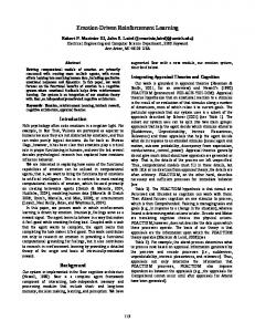
(b) τ = 1.0 ∗
Fig. 1. Random MDP results.Shown is the average value of maxs,a |Q∗ − Qπˆ |.
4
Experimental Results
In this section we provide experiments illustrating how the performance of model-based methods varies with the amount of available experience and the quality of the partition. 4.1
Empirical Results for Randomly Generated Finite MDPs
The first experiments use randomly generated MDPs with finite state spaces, in which the model can be represented exactly. This allows us to ignore the effect of the quality of the partition and to focus on how the number of samples used to learn the model affects performance. We used a suite of MDPs with randomly generated transition and reward models. In order to produce environments that are more similar to typical RL tasks, some of these MDPs were designed to have a 2D lattice-like structure. The lattice has n2 states, where n is the length of the side, and four actions. Each state has a set of four neighboring states; the effect of each action when the environment is fully latticial is to take the agent to the corresponding neighboring state with probability 0.8; with probability 0.2, there is a uniformly random transition to one of the corresponding next state’s neighbors. The degree to which the transition model is lattice-like depends on the parameter τ ∈ [0, 1], which denotes the probability that an action will behave randomly. Thus, with probability τ the effect of the action is to take the agent randomly to one of m successor
states (the successor states for each state are uniformly randomly chosen in advance). For example, τ = 1 means that the lattice structure has no effect. The reward for each state-action pair is 0 with probability 0.9; with probability 0.1, the reward is drawn uniformly from [0, 1]. The discount factor γ = 0.95. The model is learned using maximum likelihood with the uniform and loop-back priors as described in section 2. The data is generated by sampling state-action pairs uniformly randomly, then sampling the next state from the true distribution. We computed πˆ∗ , the optimal policy for the learned model, by doing value iteration with the learned transition model and the (known) reward function. Value iteration was run on the learned model until the maximum change in the state-action values was ≤ .000001. Then we evaluated the performance of πˆ∗ in the real environment, by using ˆ∗ policy policy iteration. More precisely, we computed maxs,a |Q∗ − Qπ |, where Q∗ is the correct optimal policy. As a baseline, we compared against the well-known SARSA algorithm (Sutton and Barto, 1998) an on-line, on-policy, model-free algorithm. We ran SARSA for the same number of steps as the number of samples collected and we used the same scheme to compare the policy produced by SARSA to the optimal policy. The learning rate α was set to 0.001 for SARSA (as it seemed to perform best in initial experiments), and we used ε-greedy exploration with ε = 0.1. The results for 64 states and connectivity m = 5 with τ = 0.0 and τ = 1.0 are shown in Figure 1. The results were averaged over 60 independent runs, each with a different random MDP. The error bars were vanishingly small and were removed for clarity. ˆ∗ As expected, the value of maxs,a |Q∗ −Qπ | decreases as the number of data samples increases. With little or no data, the performance is different for the two initial models, but this effects disappears as the agent starts to see samples for all state-action pairs. With no data, the algorithm has the same performance as an agent that always chooses the action with the highest immediate reward. We also notice that the overall shape of the graph is similar for the lattice-like structure and the completely random MDP. The model-based approach clearly outperforms the SARSA baseline. This can be largely attributed to the fact that SARSA only gets on-policy data and only does one update per sample. We also experimented with batch experience-replay methods. The results are not shown here, since the learning curves were similar to those of the model-based methods, as is to be expected for discrete MDPs. The effect of the initialization for the model seemed innsignificant. Next we examine the effect of varying the size of the number of states on the speed of convergence. We created random MDPs with varying values of |S| ∈ (20, 50, 100, 200), four actions and m = |S|/10. For each value of |S|, we plotted the number of samples ˆ∗ required in order to have maxs,a |Q∗ − Qπ | < 0.5 for more than 90% of the MDPs. The results are averaged over 20 random MDPs of each size and are shown in Figure 2. Our results displayed a linear trend in the number of samples required to obtain a good policy as the number of states increases, the number of actions is kept fixed and the connectivity is kept to a fixed fraction of the number of states. More such experiments would confirm whether this is indeed a general trend. We also looked at how the estimated model improves with the number of samples. In Figure 3, we show how the L1 error of the estimated model decreases with the number of samples. Plugging these errors into the bound in Theorem 1 results in values that are
10000
9000
8000
7000
6000
5000
4000
3000
2000
1000
20
40
60
80
100 120 140 Size of State Space
160
180
200
∗
Fig. 2. Number of samples required for maxs,a |Q∗ −Qπˆ | < 0.5 in more than 90% of the randomly generated MDPs.
far from the empirical performance of πˆ∗ ; this, however, is expected for bounds of this type.
2 Model:Uniform Model:Loop−back
1.8
1.4
1.2
1
s,a
max |P(s‘|s,a) − P∧(s‘|s,a)|
1.6
0.8
0.6
0.4
0.2 0
0.5
1 Data Exploration Steps
1.5
2 4
x 10
Fig. 3. The L1 error in estimating the model.
4.2
Empirical Results for MDPs with Continuous State Space
We tested the algorithm on a modification of the well known Mountain Car domain (Moore, 1990). The left and right actions were made stochastic, with Gaussian noise added with standard deviation σ = .001. The goal region was the standard Mountain
Car goal of x ≥ 0.5, with the added restriction that the agent stops at the top of the mountain (|v| < 0.01). Reward was -1 everywhere except for 0 at the goal, and a reward of -100 was given if the agent exceeded 10000 time steps without reaching the goal. The discretization divided the state space and velocity space into 40 partitions each, giving a total of 1600 partitions. Value iteration was run on the learned model until the maximum change in the state-action value function was ≤ .0001, up to a maximum of 100 steps. We ran our algorithm with both model initialization methods. The average return of the resulting policy was estimated by averaging 10 independent runs of Monte Carlo policy evaluation on the underlying environment, where each episode was run for a maximum of 10000 steps. We compare our policy to the policy obtained by running SARSA with α = 0.02 and ε = 0.1 until convergence. The results are averaged over 20 independent trials and are shown in Figure 4. The behavior is qualitatively very similar to that of the random MDPs.
Converged SARSA Model:Uniform Model:Loop−back
0
1
2
3
4
5
Data Exploration Steps
6
7 4
x 10
Fig. 4. Results for stochastic Mountain Car with stopping at the top. MBRL converged to a good estimate with about 10 samples per state-action pair on average.
4.3 Discussion The empirical results provide intuition with respect to the amount of data required in order to compute a good policy, when that policy is computed using the model-based approach with a discrete model. In the experiments, we considered a favorable scenario by assuming that we can sample each state-action pair uniformly. We chose this distribution as it is guaranteed to sample each state-action pair, which is required for satisfying Theorem 1. In practice, the distribution will likely not be uniform, as the data is typically collected by running some policy in the environment. This can lead to situations where important regions of the state space have low probability. In fact, we have observed in experiments not reported here that not visiting some part of the state space can have hazardous effects, even if that region is not important for the optimal policy.
Note that in this case, our bound will also predict high errors, as the maximum L1 error will remain high.
5
Conclusions and future work
We presented the first sample complexity results for model-based reinforcement learning with state aggregation. Our bounds highlight the trade-off between the quality of the partition and the number of samples needed for a good approximation. There are several avenues for future work. The quality of the PAC result used to estimate the L1 error in the model can be tightened further, using Azuma’s inequality (this is an avenue which we are actively pursuing at the moment). There are several ways in which the results can be tightened. Instead of using L∞ norm, we could work with L p norm. Munos (2007) provides a theoretical analysis of approximate value iteration with the L p norm, which can be used as a step in this direction. Also, instead of using the maximum L1 error, we could likely work with a version weighted by a desired distribution. Our current approach assumes that the samples on which the model is built are drawn i.i.d. In practice, these samples may have come from experience obtained by solving a previous task. In this case, the correlation between samples must be taken into account (as in Mannor et al, 2007). Our results do not extend immediately, but can likely be adapted with more work. The general case of linear function approximation is not covered by our results. In this case, there are still open questions in the field about how to build a transition model. However, the idea of having identical feature vectors for “similar” states should still be useful.
Bibliography
Antos, A., Munos, R., & Szepesvari, C. (2007). Value-iteration based fitted policy iteration: Learning with a single trajectory. IEEE International Symposium on Approximate Dynamic Programming and Reinforcement Learning. Corrado, C. J. (2007). The exact joint distribution for the multinomial maximum and minimum and the exact distribution for the multinomial range. Ernst, D., Guerts, P., & Wehenkel, L. (2005). Tree-based batch mode reinforcement learning. Journal of Machine Learning Research, 6, 503–556. Kearns, M., & Singh, S. (1999). Finite-sample rates of convergence for q-learning and indirect methods. Advances in Neural Information Processing Systems 11. Kuvayev, L., & Sutton, R. S. (1996). Model-based reinforcement learning with an approximate, learned model. Proceedings of the 9th Yale Workshop on Adaptive and Learning Systems (pp. 101–105). Lagoudakis, M. G., & Parr, R. (2003). Least-squares policy iteration. Journal of Machine Learning Research, 4, 1107–1149. Lin, L.-J. (1992). Self-improving reactive agents based on reinforcement learning, planning and teaching. Machine Learning, 8, 293–321. Mannor, S., Simester, D., Sun, P., & Tsitsiklis, J. N. (2007). Biases and variance in value function estimates. Management Science, 53, 308–322. Moore, A., & Atkeson, C. (1995). The parti-game algorithm for variable resolution reinforcement learning in multidimensional state-spaces. Machine learning, 21. Moore, A. W. (1990). Efficient memory-based learning for robot control. Doctoral dissertation, Cambridge, UK. Munos, R., & Moore, A. (2002). Variable resolution discretization in optimal control. Machine learning, 291–323. Puterman, M. L. (1994). Markov decision processes: discrete stochastic dynamic programming. Wiley. Strehl, A. L., Li, L., & Littman, M. L. (2006). Incremental model-based learners with formal learning-time guarantees. Proceedings of the 22nd UAI. Strehl, A. L., & Lihong Li, M. L. L. (2006). Pac reinforcement learning bounds for rtdp and rand-rtdp. Proceedings of AAAI’06 Workshop on Learning For Search. Sutton, R. S., & Barto, A. G. (1998). Reinforcement learning: An introduction. MIT Press.
Appendix A
Proof of Lemma 1
Using the triangle inequality: ∗
∗
π∗
π∗
kQπΩ − Q∗ k∞ ≤ kQπΩ − QΩΩ k∞ + kQΩΩ − Q∗ k∞ .
(2)
First we bound the second term, relating the optimal value function of MΩ to the optimal value function of M. Let us arbitrarily choose a partition ω ∈ Ω and a state s ∈ ω. We use the following Bellman equations: Q∗ (s, a) = R(s, a) + γ and
π∗
QΩΩ (ω, a) = RΩ (ω, a) + γ
Z S
∑ 0
P(s0 |s, a) max Q∗ (s0 , a0 )ds0 a0
π∗
ω ∈Ω
PΩ (ω0 |ω, a, d) max QΩΩ (ω0 , a0 ). a0
π∗
Let ∆1 = |Q∗ (s, a) − QΩΩ (ω, a)|. Since we assumed that the reward R(s, a) depends only on the partition ω(s), we have ∆1 = γ|
Z S
−
P(s0 |s, a) max Q∗ (s0 , a0 )ds0 a0
∑ 0
π∗
0
ω ∈Ω
PΩ (ω |ω, a, d) max QΩΩ (ω0 , a0 )| a0
π∗
R
By adding and subtracting S P(s0 |s, a) maxa0 QΩΩ (ω(s0 ), a0 )ds0 inside the absolute value, and applying the triangle inequality, we obtain ∆1 ≤ A + B where A = γ|
Z S
π∗
P(s0 |s, a)[max Q∗ (s0 , a0 )ds0 − max QΩΩ (ω(s0 ), a0 )]ds0 | and a0
π∗
a0
B = γ| max QΩΩ (ω0 , a0 )[ a0
∑ 0
Z
0 ω ∈Ω ω
P(s0 |s, a)ds0 −
∑ 0
ω ∈Ω
PΩ (ω0 |ω, a, d)]|.
By using Jensen’s inequality to move the absolute value inside the integral, upper bounding the absolute value of the value function difference by its L∞ norm, and observing that the transition density integrates to 1, we can upper bound A by π∗
A ≤ γkQΩΩ − Q∗ k∞ In order to upper bound B, we will need to re-write PΩ (ω0 |ω, a, d). Expanding the shorthand notation, we have PΩ (ω0 |ω, a, d) = P(st+1 ∈ ω0 |st ∈ ω, at = a, d) = Z
P(st+1 ∈ ω0 , st ∈ ω|at = a, d) P(st ∈ ω|at = a, d)
1 P(st+1 ∈ ω0 , st = s|at = a, d)ds P(st ∈ ω|at = a, d) ω Z 1 = P(st = s|at = a, d)P(st+1 ∈ ω0 |st = s, at = a, d)ds P(st ∈ ω|at = a, d) ω Z 1 P(st = s|d)P(st+1 ∈ ω0 |st = s, at = a, d)ds = P(st ∈ ω|d) ω =
If we denote the first factor in the integral by d(s), and we realize that we do not need to condition on d in the second factor because we know the state, we get (using the shorthand notation again) PΩ (ω0 |ω, a, d) =
1 P(ω|d)
Z ω
d(s)P(ω0 |s, a)ds.
R 1 P(ω|d) ω d(x)dx = 1, Jensen’s inequality and the upper π∗ π∗ | maxa0 QΩΩ (ω0 , a0 )| ≤ kQΩΩ k∞ we have
Using this equation, the fact that bound
π∗
B ≤ γkQΩΩ k∞ | =
π∗ γkQΩΩ k∞ π∗
= γkQΩΩ k∞
1 P(ω|d)
Z
∑ 0
[P(ω0 |s, a) −
∑
sup |P(ω0 |s, a) − P(ω0 |x, a)||
ω ∈Ω
ω
d(x)P(ω0 |x, a)dx]|
ω0 ∈Ω x∈ω
∑ 0
1 P(ω|d)
¯ ¯ sup ¯P(ω0 |s, a) − P(ω0 |x, a)¯
Z ω
d(x)dx|
ω ∈Ω x∈ω
Taking the supremum over states and maximum over actions and partitions we get π∗
π∗
π∗
kQ∗ − QΩΩ k∞ ≤ γkQ∗ − QΩΩ k∞ + γkQΩΩ k∞ ¯ ¯ max sup ∑ sup ¯P(ω0 |s, a) − P(ω0 |x, a)¯ a,ω s∈ω 0 ω ∈Ω x∈ω
hence γ π∗ π∗ kQ∗ − QΩΩ k∞ ≤ kQΩΩ k∞ 1−γ ¯ ¯ 0 ¯ max sup ∑ sup P(ω |s, a) − P(ω0 |x, a)¯ . a,ω s∈ω 0 ω ∈Ω x∈ω ∗
(3)
π∗
Now let us bound kQπΩ − QΩΩ k∞ , which relates the performance of π∗Ω in MΩ (the MDP where we will learn it) to its performance in M (the MDP where we wil apply it). We will not use the optimality Bellman equations because π∗Ω is not optimal in M. Instead, we will use the standard policy-based Bellman equations, where we do not sum π∗ over actions because π∗Ω is deterministic (being the greedy policy w.r.t. QΩΩ ). Thus, we have: π∗
QΩΩ (ω, a) = RΩ (ω, a) + γ
ω ∈Ω
and ∗
π∗
∑ 0
QπΩ (s, a) = R(s, a) + γ
Z
PΩ (ω0 |ω, a, d)QΩΩ (ω0 , π∗Ω (ω0 ))
∗
S
P(s0 |s, a)QπΩ (s0 , π∗Ω (s0 )).
(π∗Ω (s) for a state s will be defined as π∗Ω (ω), where ω is the partition that includes s). At this point, we can use the same calculations as the one above, since we can still
π∗
∗
∗
bound QπΩ (s, π∗Ω (s)) by kQΩΩ k∞ and, if s ∈ ω, we can upper bound |QπΩ (s, π∗Ω (s)) − π∗Ω
π∗Ω
QΩ (ω, π∗Ω (ω))| by kQ∗ − QΩ k∞ . Thus, we have, exactly as above, ¯ ¯ ∗ γ π∗ π∗ kQΩΩ − QπΩ k∞ ≤ kQΩΩ k∞ max sup ∑ sup ¯P(ω0 |s, a) − P(ω0 |x, a)¯ . a,ω 1−γ s∈ω ω0 ∈Ω x∈ω
(4)
Inserting equations 3 and 4 into 2 completes the proof of the theorem.
B
Proof of Lemma 2
A good starting point for our proof is provided by the following result, a direct adaptation of Lemma 1 on page 13 of “Non-parametric Density Estimation: The L1 view” by Devroye and Gy¨orfi (1985): Lemma 3. If each state-action pair (s, a) is visited N(s, a) times then, for any ε ∈ (0, 1), if N(s, a) ≥ 20|S|/ε2 we have ° ° 2 ˆ a) − P(·|s, a)°1 ≥ ε) ≤ 3e−N(s,a)ε /25 . Pr(°P(·|s, Note that Lemma 3 only applies to the transitions starting from a single state, whereas we wish to bound the maximum of the L1 distances starting from all states° and actions. ° ˆ Before we move on to doing that, let us define ∆s,a = °P(·|s, a) − P(·|s, a)°1 . Assuming that we have m total samples (for all state-action pairs), we have P(max ∆s,a ≥ ε) = 1 − P(max ∆s,a ≤ ε) s,a
s,a
Next we marginalize over all possible values of N. We denote the domain of N by D(N), and the set containing all possible choices of N such that each component is bigger than some z by M(z). Using the additional notation F = P(maxs,a ∆s,a ≤ ε), we have F = P(∀s, a, ∆s,a ≤ ε) = ∑ P(∀s, a, ∆s,a ≤ ε|N = x)P(N = x) x∈D(N)
=
∑
"
≥
∑
s,a
"
∑
#
∏ P(∆s,a ≤ ε|N(s, a) = x(s, a))
∑ ∏(1 − 3e
x∈M(z)
≥
s,a
"
P(N = x)
x∈M(z)
≥
∏ P(∆s,a ≤ ε|N(s, a) = x(s, a))
P(N = x)
x∈D(N)
#
−N(s,a)ε2 /25
# ) P(N = x)
s,a
(1 − 3e−zε
2 /25
)|SkA| P(N = x)
x∈M(z)
= (1 − 3e−zε
2 /25
)|SkA| P(min(N) ≥ z)
In the equations above, x(s, a) is the component of x corresponding to state s and action a. Also, because we applied Lemma 3, we need to have z ≥ 20|S|/ε2 .