Data-Flow Oriented Visual Programming Libraries for ... - CiteSeerX

Data-Flow Oriented Visual Programming Libraries for Scientific Computing Joseph M. Maubach and Wienand Drenth Technical University of Eindhoven, Faculty of Mathematics and CS, Scientific Computing, Postbus 513, NL-5600 MB Eindhoven, The Netherlands {maubach, drenth}@win.tue.nl

Abstract. The growing release of scientific computational software does not seem to aid the implementation of complex numerical algorithms. Released libraries lack a common standard interface with regard to for instance finite element, difference or volume discretizations. And, libraries written in standard languages such as FORTRAN or c++ need not even contain the information required for combining different libraries in a safe manner. This paper introduces a small standard interface, to adorn existing libraries with. The interface aims at the – automated – implementation of complex algorithms for numerics and visualization. First, we derive a requirement list for the interface: it must be identical for different libraries and numerical disciplines, support interpreted, compiled and visual programming, must be implemented using standard tools and languages, and adorn libraries in the absence of source code. Next, we show the benefits of its implementation in a mature (visual) programming environment [1], [2] and [3]), where it adorns both public domain and commercial libraries. The last part of this paper describes the interface itself. For an example, the implementational details are worked out.

1

Introduction

This paper introduces techniques for the construction of software libraries which aid the implementation of complex numerical algorithms. Its focus is on the unaltered reuse of existing public domain and commercial libraries such as for instance packages from www.netlib.org: The Linear Algebra Package LAPack [4], FFTPack [5], Piece-wise Polynomial Package PPPack [6], Templates [7], etc. This reuse of scientific numerical software is achieved without the definition of a complete across-libraries communication language as in Open-Math [8] and MathML [9]. Instead, we adorn parts of existing standard-lacking numerical libraries with a minimal but powerful interface, ensuring fast communication in a standard computer language. The operations we interface are in general more

2

Joseph M. Maubach, Wienand Drenth

complex than the basic operations in [10], [11], and our interface is less complex than the one published in [12]. In section 3, we demonstrate how to adorn existing libraries with an interface, which satisfies at least the following so-called use-requirements: The interface should be similar across different numerical packages and disciplines, must enable and stimulate all of interpretation/compilation/visual programming, must be generated in the absence of the original source code, must be formulated in a wide-spread computer language, and must be built using a standard tools. Whenever possible, existing de facto fundamental data standards must be supported: matrices in MATLAB [13] and a free clone octave [14], matrices and vectors in Open-Math [8] and LATEX [15] (both matrix and table format), lists in Mathematica [16] and a free clone Maxima [17] various dataset formats of VTK [18], Open Inventor [19], OpenGL [20] and java3d [21]. Each of the proposed use-requirements has its advantages. To mention a few: A similar interface aids the implementation of complex algorithms, interpretation is convenient, complication ensures speed, and visual programming provides application-level overview (see [1], [22]) as well as visualization/solver interaction (see [1] and [3], but also the use-cases presented in [12] and the references cited therein). Building an interface from a library in the absence of source code is a requirement for the reuse of a commercial library ([23], [24], [25], etc.). Using a wide-spread standard fast language turns out to be feasible, so it is a must. The remainder of this paper is composed as follows. First, section 2 shows how the to be introduced interface can be used to implement complex numerical algorithms in a rather convenient manner. The interface itself is presented in section 3, which also provides an example implementation.

2

Data-Flow oriented Scientific Computing

Because our proposed interface must aid the implementation of complex numerical problems, we first examine the nature of numerical complex. We distinguish two categories of complex complex numerical problems. We call a numerical complex problem global, if a range of numerical problems for which each a software solution exists, is combined into one. An example would be a transient problem involving multiple conservation equations in a moving domain, where different state variables and equations have to be discretized using different methods such as finite element and volume techniques. The second category of complex problems is called local. An example of this category is a single non-trivial discretization or iterative solver which requires various types of input and output data. The distinction into local and global complex problems is of course relative, so all techniques used to solve the local ones, solve the global ones – see [1] for detailed information on the global case.

Data-Flow Oriented Visual Programming Libraries for Scientific Computing

3

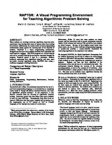
For the remainder of this paper, our example of a complex numerical problem is the leading-order problem for the solidification of an amount of molten material flowing past a relative cold solid wall from [26], based on [27] and [28]. As described in more detail in [29], an axis-symmetric splash of metal moves along the inside wall of a cylinder as in figure 3. The related x and y coordinate-directions are along and perpendicular to the inside wall. The metal splash is part molten (liquid) and part solid: Its total height is φ(x, t), and the height of the internal solid/liquid interface is 0 ≤ ψ(x, t) ≤ φ(x, t). The temperature is denoted by θ(x, y, t). In different subdomains, the splash’s movement is determined using: The conservation of mass:

momentum:

∂ ∂ψ ∂φ + (uφ) = − ; ∂t ∂x ∂t

(1)

∂ ∂ 2 ∂ψ (uφ) + (u φ) = −u , ∂t ∂x ∂t

(2)

and energy: ∂θ ∂ ∂ + (uθ) + ∂t ∂x ∂y

∂θ {(uψ)x − ux y} θ − D = 0, ∂y

(3)

in combined with initial, Dirichlet, Neumann, Robin, and Stephan conditions. The discretization and related iterative solution algorithm we use in our example program is presented in [29]). This problem is complex at a global level and also at a local level: φ and ψ are represented using splines (PPPack), are visualized super-imposed on a cylinder (VTK, Open Inventor (OI)), and are obtained solving systems of equations (LAPack and SEPRAN). Figure 1 shows part of an implementation, loaded into the NumLab visual programming environment (see [1]). The implementation uses functions (modules) from different libraries including LAPack, PPPack, SEPRAN, VTK, OI, etc., as well as operating system commands: The mpeg module. As most numerical programs, the program in figure 1 can be divided into three parts: (1) The part which reads the input and performs the numerical computations; (2) The part which visualizes the computed results; and (3) the post-processing part which writes the output. Figure 2 shows the automatically built editors which can be used to enter values of arguments which are not connected. Figure 3 depicts a VTK module, which shows the initial shape of the splash of metal, superimposed with graphical operations onto the inside of a cylinder wall. Both so-called viewers offer solid, hidden-line, wire-frame and other representations, as well as interactive 3-d manipulation of the visualized objects. In order to understand the program related to figure 1 the depicted visible graphical elements must be explained. Each rectangle such as MIteration is a graphical representation of a function, using the interface proposed in section 3. For

4


1

2

3

Fig. 1. A program which calculates deformations caused by laser drilling


5

the sake of convenience, we call this representation also module. Within each module, we distinguish bottom and a top area. Modules have either input or output arguments (input/output are not part of a function’s interface). Each of its arguments made available via the interface description, is mapped to a small colored rectangular area at the top or bottom the module. Using standard data-flow terminology, these small rectangles are called ports. Different builtin argument types are colored in a different manner, all pointers and derived types are colored using a default (green). The function’s interface determines the position of each argument port. Next, each port is either connected, or behind the

Fig. 2. The user provides defaults to the modules using an automatically built editor

scenes a default value is used. Output is connected to input using the mouse (click on bottom port, drag to top port and release. The connection is established when the data types concur). Default values are altered using a graphical user interface which is generated from the function’s interface, and which pops up when selected (clicking on the module reveals a list of options, amongst which is Edit). Building complex numerical algorithms with NumLab is convenient because of the libraries LAPack, EigPack, SEPRAN, PPPack, VTK, OI which have been interfaced and because of those which have been added (data-types, dataexchange in MATLAB/Mathematica/Open-Math/LaTeX/VTK/other formats, discretized ordinary and partial differential related operators). All implementations such as LAPack have been interfaced for that part which covers the currently conducted research. This means that about half a million lines of code out of 4 million is interfaced, covering about 1000 modules,

6


Fig. 3. The contour φ(x, 0) of the liquid metal on the cylinder wall

3

The construction of data-flow oriented libraries

With the NumLab environment from the previous section kept in mind, we show how to interface existing libraries such that all promised use-requirements are met. Our techniques uses design patterns (inheritance, proxies) such as in [31], [32], [33] and [34]. First, we regard the choice of language for the implementation of the interface. To begin with, because of all toolboxes must offer a similar visual programming interface, a common language must be used. Next, the use-requirement that all toolboxes can also be interpreted, requires the use of a common language which can be interpreted. Not introducing a new language implies using an existing one, and using source-libraries means that the common language must be a kind of union of all source-libraries’ languages (Pascal, FORTRAN, c, c++). Thus, the interpreter/compiler must be able to distinguish all related data types. With the NumLab environment from section 2 kept in mind, we assume that the common language is a large subset of c++: That subset of c++ which cint c++ interpreter can interpret – see the manual of [35]. The interpreter cint can interpret most c++ programs, even when templates are used in combination with compiled code. Now, we introduce the interface structure (implementation) itself. We restrict ourselves to interfaces for fortran libraries because most of the numerical implementation we use are written in fortran. Also c++ code can be adorned with our interface (using proxies instead of direct inheritance from class-level to modulelevel below), but the description falls outside the scope of this paper. The first layer is the so-called source-layer. It contains (the functions from) the libraries which the user wants to use. Assume we want to use the compiled


7

function f(z, x), in combination with documentation which describes that both the input argument x (only read from) and the output argument z (only written into). For the sake of a simple presentation we assume that both arguments are documented to be of type X. The source of the documentation (include file, reference manual, etc.) is irrelevant. For languages such as c++, input and output can be deduced when the keyword const is used in a proper manner. However, using this keyword at the right moment is difficult and often forgotten, so even for c++ program extra documentation is recommended in principle. Other languages such a FORTRAN lack the const feature and absolutely require related documentation. The second and middle layer is called class-layer. It contains one c++ class for each function in the bottom layer. The class has a signature which is derived from the source. Assuming we know which variable is input and which one output, the class which interfaces the source f() is called class cf, and defined as follows class cf { public: cf(); cf(X &z, const X x); int callback(X &z, const X x); void print(ostream &) const; }; ostream &operator(ostream &, const cf &); The second constructor uses the call-back on the function callback() which returns value Ok if all went fine during its call-back to f() , and returns value NotOk if the call to f() somehow failed. If for instance f() was a higher level LAPack function, its success or failure could be detected inspecting the output argument with name info. The print() and output methods