To minimize idle times of the CPU, caches are used to speed ... codes are not cache-aware and hence exploit less than 10 percent of the peak performance of.
DATA LOCALITY OPTIMIZATIONS TO IMPROVE THE EFFICIENCY OF MULTIGRID METHODS
Christian Weiß and Hermann Hellwagner Institut f¨ur Informatik Technische Universit¨at M¨unchen D-80290 M¨unchen, Germany Ulrich R¨ude Institut f¨ur Mathematik Universit¨at Augsburg D-86135 Augsburg, Germany Linda Stals Department of Mathematical Sciences, University of Bath Bath, BA2 7AY, UK
SUMMARY
Current superscalar microprocessors are able to operate at a peak performanc e of up to 1 GFlop/sec. However, current main memory technology does not provide the data needed fast enough to keep the CPU busy. To minimize idle times of the CPU, caches are used to speed up accesses to frequently used data. To exploit caches, the software must be aware of them and reuse data in the cache before it is being replaced. Unfortunately, all conventional multigrid codes are not cache-aware and hence exploit less than 10 percent of the peak performance of cache based machines. Our studies with linear PDEs with constant coefficients show that it is possible to speed up the execution of our multigrid method by a large factor and hence solve a Poisson’s equation with one million unknowns in less than 3 seconds. The optimized reuse of data in the cache allows us to exploit 30 percent of the peak performance of the CPU, in contrast to mgd9v for instance, which achieves less than 5 percent on the same machine. To achieve this, we used several techniques like loop unrolling and loop fusion to better exploit the memory hierarchy and the superscalar CPU. We study the effects of these techniques on the runtime performance in detail. We also study several tools which guide the optimizations and help to restructure the code.
CPU
Capacity
Bandwidth
Latency
Registers
256 Bytes
24000 MB/s
2 ns
1. Level Cache
8 KBytes
16000 MB/s
2 ns
2. Level Cache
96 KBytes
8000 MB/s
6 ns
3. Level Cache
2 MBytes
888 MB/s
24 ns
Main Memory
1536 MBytes
1000 MB/s
112 ns
Swap Space on Disk
Figure 1: Memory Hierarchy of the DEC PWS 500au A21164
1. INTRODUCTION
Over the last 10 years the speed of microprocessors has increased at a rate of around 80 percent per year [1]. Through the use of pipelining, fast add-and-multiply operations and other techniques, a single RISC processor can now reach a peak performance of around 1 GFlop/sec. The continuing evolution is expected to yield further performance increases of estimated 60 percent annually [2]. Relative to the computational speed, the memory access times and throughput have increased very slowly, only at a rate of 5-10 percent per year [1], so that the typical peak main memory bandwidth of workstations now is still much smaller than 1 GByte/sec [3]. At peak CPU speed, however, 24 times as much would be necessary to support (DAXPY-type) vector operations. This phenomenon is often called “hitting the memory wall” [4]. A common approach to at least mitigate its effects is to use a memory hierarchy. There are many different ways of implementing this concept, but the consistent theme is that there is a large, cheap, slow memory at the bottom of the hierarchy and a small, expensive, high speed memory at the top of the hierarchy. This high speed memory is called a cache and is intended to contain copies of main memory blocks to speed up accesses to frequently needed data. An example of a memory hierarchy with three levels of caches is shown in figure 1. However, because of the limited size, caches can only hold copies of the recently used data. To exploit caches, the software must be aware of them and reuse data in the cache before it is being replaced. The effectiveness of data locality optimizations has been well demonstrated in LAPACK [5], a linear algebra package for dense matrices, and FFT algorithms (see for example [6]). However, little work in that direction has been done for iterative techniques and research into more advanced iterative methods such as multigrid has only just begun [7; 8]. The difficulty with iterative methods can be seen in the following example. The program mgd9v [9] is a robust Fortran 77 multigrid program designed to solve 2D elliptic partial differential equations and is optimized for vector computers. We compiled the program with aggressive optimizations enabled and solved Poisson’s equation on a 513 � 513 grid so that the L2 norm of the residual was less than 4 � 10?8 . The obtained results on a SGI Power Indigo based on a 75 MHz clocked MIPS R8000 CPU (300 MFlops/sec), a SGI Origin 2000 node based on a
Time MFlops/sec % Peak R8000 19.7 sec 13.8 4.6 R10000 6.2 sec 43.7 11.2 DEC 7.2 sec 36.6 3.6 Table 1: Solving Poisson’s Equation with mgd9v
195 MHz clocked MIPS R10000 CPU (390 MFlops/sec) and a DEC PWS 500au based on a 500 MHz clocked Alpha 21164 (1 GFlop/sec) are shown in table 1. On all machines, the program only achieves a small fraction of the peak performance. However, on the fastest machine - the DEC PWS 500au - the program is even less efficient than on the SGI Origin node. An analysis with tools like perfex [10] and DCPI [11] reveals that the limiting factor for iterative methods is not the numerical computation but memory access. As the above example indicates, the efficiency of these methods may even decrease with increasing processor speed. We started our data locality studies with a straightforward implementation of the multigrid method in C assuming that the finite difference stencil is constant on each grid level. This restricts the discussion in the paper to linear PDEs with constant coefficients, though clearly many of the basic ideas can be carried over to more general situations. We consider the finite difference approximation of Poisson’s equation defined on the square domain with Dirichlet boundary conditions. Consistent with the multigrid algorithm, we use a nested sequence of uniform grids M1 � M2 � � � � � Mn , with the grid spacing on level k being hkx = hky = 2?k . In this paper we will use the compact 9-point Mehrstellen-stencil. We implemented a Vcycle and a FMV scheme and applied several in-cache1 and out-of-cache2 optimizations to the smoother and the overall algorithm and studied the effects on the performance on a SGI Power Indigo based on a 75 MHz clocked R8000 CPU. In this paper we only present the results for the V-cycle scheme. The results for the FMV scheme as well as results for a 5-point stencil version can be found in [12]. The remainder of the paper is structured as follows. Section 2 discusses a cache-oriented red-black Gauss Seidel smoother. Section 3 explains how the components of a V-Cycle algorithm are combined to a cache-oriented multigrid program and section 4 provides some conclusions.
2. RED-BLACK GAUSS SEIDEL
We use the red-black Gauss Seidel to smooth the equations on each grid level. As the smoother is one of the most computationally expensive parts of the multigrid algorithm it shall be described in some detail. Figure 2 shows the MFlops/sec rate for different implementations of the red-black Gauss Seidel algorithm. The line labeled red black (1) is the result of what we would consider to 1 In-cache means that
the amount of data is small enough to fully fit in the cache. means that the total amount of data is too large to fit in the cache so that parts of the data need to be copied more than once from main memory into the cache. 2 Out-of-cache
180 red black(1) red black(2) red black(4)
160 140
MFlops/sec
120 100 80 60 40 20 0 4
16
64 grid size
256
1024
Figure 2: MFlops/sec Rate for Different Implementations of Red-Black Gauss Seidel.
be a standard implementation of the red-black Gauss Seidel method. The lines labeled red black (2) and red black (4) were obtained by using an optimization technique similar to loop unrolling (see figure 3 or [13] for a more detailed description of the technique). Clearly this technique is effective in improving the in-cache performance as it more then doubles the maximum MFlops/sec rate. The reason for this is that loop unrolling can introduce additional instruction level parallelism and hence help to improve the utilization of the functional units of superscalar CPUs[14]. However the out-of-cache performance is not affected at all. Figure 2 clearly shows the cache effect for small grids. Once the grid is too large to fit in the cache ( > 256 � 256), the performance decreases dramatically. The reason for this is that a complete update performs two global sweeps through the whole grid. Assuming that the grid does not fit in the cache, the data of the lower part of the grid is no longer in the cache after the red update sweep because the data was replaced by the grid points in the upper part of the grid. Hence, the data must be loaded from the slower main memory into the cache again. Doing this they replace the upper part of the grid points in the cache and as a consequence they have to be loaded from main memory once more. It may seem unnecessary to spend time on improving the in-cache performance when we are mainly interested in the results for large grids, however all methods of improving the out-ofcache performance involve some sort of blocking technique. That is, we try to break the large grids up into smaller grids. So if the performance for the small grids is poor, the performance for the large grids will be poor as well. When implementing the standard red-black Gauss Seidel algorithm, the usual practice is to do one complete sweep of the grid from bottom to top updating all of the red nodes and then one complete sweep updating all of the black nodes. The first point to note is that as a red node in row i is updated the black node in row i-1 directly underneath it may also be updated. If a 9-point stencil is placed over one of the black points (see figure 4) then we can see that all of the red points it touches are up to date (as long as the red node above it is up to date).
— Update w. loop unrolling (factor 2) — // red nodes: do i = 1 , n-1 do j = 2-i%2 , n-1 , 4 Relax( u(i,j) ) Relax( u(i,j+2) ) endo endo
— Standard Update — // red nodes: do i = 1 , n-1 do j = 2-i%2 , n-1 , 2 Relax( u(i,j) ) endo endo // black nodes: do i = 1 , n-1 do j = 1+i%2 , n-1 , 2 Relax( u(i,j) ) endo endo
// black nodes similar
Figure 3: Simplified Loop Unrolling in the Case of Red-Black Relaxation
11 00
i i-1 i-2
11 00
11 00
111 000 000 111 000 111
black point red point
11 00
Figure 4: Data Dependencies in Red-Black Relaxation Algorithm
180 red black(4) fused (1, 1) fused (2, 2) fused (4, 0)
160 140
MFlops/sec
120 100 80 60 40 20 0 4
16
64 grid size
256
1024
Figure 5: MFlops/sec Rate for Different Implementations of Red-Black Gauss Seidel.
i+1
111 000
i i-1
11 00
i-2 i-3
11 00
11 00 11 00
11 00 111 000 11 00
11 00 11 00
11 00 11 00 11 00
i+1
111 000
i i-1
11 00
111 000 11 00
i-2 i-3
11 00
11 00 11 00
11 00 111 000 11 00
11 00 11 00
11 00 11 00 11 00
111 000 11 00
Figure 6: Example of fusing two sweeps together. Each circle around a node shows how many times it has been updated.
Consequently, we work in pairs of rows; once all of the red nodes in one row have been updated, all of the black nodes in the previous row are updated. So instead of doing a red sweep and then a black sweep, we just do one sweep of the grid updating the red and black nodes as we move through. The line labeled fused(1,1) in figure 5 shows how this can improve the MFlops/sec rate. The consequence is that the grid must be transfered from main memory to cache only once per update sweep instead of twice, as long as at least four lines of the grid fit in the cache. Three lines must fit in the cache to provide the data for the update of the black points and one additional line for the update of the red points in the line above the three lines. In the next step we melt the sweeps together. For example, instead of doing two sweeps, and updating the nodes once during each sweep, we do one sweep and update the nodes twice. Because of the complex data dependencies, it is difficult to describe this in detail, therefore we refer the reader to [12] for a more thorough discussion and just try to present the basic ideas here. Loosely speaking we copy a section of the grid into the cache and then update the nodes as many times as is allowed without violating the data dependencies (as defined by the standard red-black Gauss Seidel algorithm). We start in a situation where we have updated some of the rows once (see figure 6 left side). Before we continue the first update sweep in row i we are able to update the red points in row i-3 the second time. Once all of the red nodes in row i have been updated, all of the black nodes in row i-1 can be updated. Then all red nodes in line i-2 are updated the second time and as a consequence also the black nodes in row i-3 are updated the second time (situation in figure 6 on the right side). Then we update the red points in row i+1 and cascade down three rows as described and so on. The technique can be generalized so that the nodes can be updated � times in one sweep through the grid obtaining the same results we would get if � sweeps of the standard red-black Gauss Seidel algorithm were applied. The line labeled fused(2,2) in figure 5 shows the result of two calls to the melt algorithm with � = 2. We simulate the case in the multigrid algorithm where we do a pre and post smoothing sweep with the number of both the pre and post smoothers being equal to 2. The line labeled fused(4,0) in figure 5 shows what happens if we melt � = 4 sweeps together. It is interesting to note that there is the same number of operations in fused(2,2) and in fused(4,0), but the MFlops/sec rate for fused(4,0) is far better. This is because it makes fewer sweeps through the grid (1 compared to 2) and thus reduces the number of times the data must be copied into the cache.
180 optimized RB melt(2, 2) melt(3, 3) melt(4, 4)
160 140
MFlops/sec
120 100 80 60 40 20 0 4
16
64 grid size
256
1024
Figure 7: MFlops/sec Rate for Different Implementations of the V-cycle.
3. V-CYCLE
As mentioned above, we use the red-black Gauss Seidel algorithm as a smoother in the multigrid algorithm. The interpolation operator is bilinear interpolation and the restriction operator is given by the transpose of the interpolation operator. The multigrid algorithm used here is the standard V-cycle. To optimize the residual and restriction calculations we used a loop unrolling technique similar to the one used for red-black Gauss Seidel (see [12]). The results for two pre and post smoothers is given by the line labeled optimized RB in figure 7. This step is designed to improve the in-cache performance. When the different components of the multigrid algorithm are put together, the performance again drops dramatically when the data does not fit in the cache anymore. The various operators used in the multigrid method can be grouped into pre coarse grid operations (smoother, residual calculation and restriction) and post coarse grid operations (interpolation and smoother). To improve the out-of-cache performance, we melted the pre coarse grid operations together and the post coarse grid operations together. The other lines in figure 7, labeled with melt(�1 ,�2 ), show the results with �1 pre smoothers and �2 post smoothers. Melting the operations together is a non-trivial task, but it does pay off by the increased out-of-cache performance. The reason why the MFlops/sec rates are improved as the number of pre and post smoothers is increased is that more work is done before moving down to the coarse grids. When the algorithm moves down to the coarse grids, any fine grid information is evicted from the cache. These results are interesting because increasing the number of pre and post smoothers also increases the convergence rate and thus gives a more efficient algorithm. The pre coarse grid operations are melted by smoothing over p rows, then calculating the residual for p rows, and finally applying the restriction operator to p rows. The size of p is
350 unrolled RB fused RB melt(2, 2) melt(3, 3) melt(4, 4)
300
MFlops/sec
250
200
150
100
50
64
128
256 grid size
512
1024
Figure 8: MFlops/sec Rate for Different Implementations of the V-cycle on a DEC PWS 500au.
unrolled RB fused RB melt (2,2)
% Cycles time MFlops/sec D-Miss Stall Execution 1.8 sec 98 53.2 26.6 1.3 sec 142 31.7 31.7 1.1 sec 162 28.6 38.5
Table 2: Performance Evaluation on a DEC PWS 500au: Where have all the cycles gone?
chosen at compile time so that p rows will fit into the cache. The melted code is simply build upon the straightforward code. However, the calculations of the restriction must lag 2 � (�1 + 1) rows behind the smoother to observe the data dependencies. The post grid operations are melted together by interpolating several coarse grid rows and then applying the post smoother. This idea is similar to the approach for the pre coarse grid operations described before. Namely, we apply the interpolation to p rows and then smooth p rows. Again, the smoother must lag two rows behind the coarse grid correction because of the data dependencies. For a more detailed discussion of the approaches see [12]. We have also done some preliminary experiments with our algorithm on a DEC PWS 500au. The results of the experiments are shown in figure 8. The line labeled unrolled RB represents the results for the V-cycle scheme without out-of-cache optimizations and two pre and post smoothers. The line labeled fused RB represents the results obtained with the out-of-cache optimized version of the smoother. The other lines represent the results for the version with melted pre and post coarse grid operations. The results are comparable to the results on the SGI Power Indigo. However, the achieved fraction of the peak performance is even smaller. Table 2 summarizes an evaluation of the code with the profiling tool DCPI [11]. The evaluation was performed while solving Poisson’s equation on a 1025 � 1025 grid with two pre and post smoothers. The cycling was stopped as soon as the L2 norm of the residual was less than
4
10?8 .
Running the unoptimized version of the code, the CPU was stalled for more than 70 percent of all cycles. 53.2 percent of all stall cycles were caused by data cache misses. Our optimizations were able to nearly halve the amount of stalls due to data cache misses. �
4. CONCLUSIONS
This article demonstrates the need for data locality optimizations for multigrid methods. Also, it introduces techniques to improve multigrid performance by restructuring the data accesses such that all data dependencies are preserved and identical results to the standard algorithm are obtained. So far, the techniques have been designed for and applied to a restricted set of problems. However, we believe that similar techniques can be applied to the core routines of more complex multigrid methods as well. Therefore, our current research ai ms to develop a more general multigrid code and extend the optimization techniques for this code. We also investigate further performance profiling tools to be able to study the effects of code transformations in more detail.
ACKNOWLEDGMENT
This research is supported by the Deutsche Forschungsgemeinschaft, project Ru 422/7-1.
REFERENCES
[1]
D. C. Burger, J. R. Goodman, and A. K¨agi. The Declining Effectiveness of Dynamic Caching for General-Purpose Microprocessors. Technical Report TR-95-1261, University of Wisconsin, Dept. of Computer Science, Madison, 1995.
[2]
D. Patterson. Microprocessors in 2020. Scientific American, September 1995.
[3]
Linley Gwennap, editor. Microprocessor Report, volume 11. MicroDesign Resources, October 1997.
[4]
Wm. A. Wulf and Sally A McKee. Hitting the Memory Wall: Implication of the Obvious. Computer Architecture News, 23(1):20–24, March 1995.
[5]
E. Anderson, Z. Bai, C. Bischof, J. Demmel, J. Dongarra, J. Du Croz, A. Greenbaum, S. Hammarling, A. McKenney, S. Ostrouchov, and D. Sorenson. LAPACK User’s Guide. Society for Industrial and Applied Mathematics, Philadelphia, PA, 1992.
[6]
D. Bailey. RISC Microprocessors and Scientific Computing. RNR Technical Report 93004, NASA Ames Research Center, March 1993.
[7]
Craig C. Douglas. Caching in With Multigrid Algorithms: Problems in Two Dimensions. Parallel Algorithms and Applications, 9:195–204, 1996.
[8]
Craig C. Douglas, Ulrich R¨ude, Jonathan Hu, and Marco Bittencourt. A Guide to Designing Cache Aware Multigrid Algorithms. In Concepts of Numerical Software, Notes on Numerical Fluid Mechanics. Vieweg-Verlag, 1998. To appear.
[9]
P. M. De Zeeuw. Matrix–Dependent Prolongations and Restrictions in a Blackbox Multigrid Solver. J. Comput. Appl. Math., 33:1–27, 1990.
[10]
Perfex - A Command Line Interface to R10000 Counters. Manual Page SGI Irix 6.4.
[11]
J.M. Anderson, L.M. Berc, J. Dean, S. Ghemawat, M.R. Henzinger, S.A. Leung, R.L. Sites, M.T. Vandevoorde, C.A. Waldspurger, and W.E. Weihl. Continuous Profiling: Where Have All the Cycles Gone? In Proceedings of the 16th ACM Symposium on Operating system Principles, St. Malo, France, October 1997.
[12]
Linda Stals and Ulrich R¨ude. Data Local Iterative Methods for the Efficient Solution of Partial Differential Equations. Technical Report MRR97-038, School of Mathematical Sciences, Australian National University, October 1997.
[13]
D.F. Bacon, S.L. Graham, and O.J. Sharp. Compiler Transformations for High-Performance Computing. ACM Computing Surveys, 26(4), December 1994.
[14]
S. Goedecker and A. Hoise. Achieving High Performance in Numerical Computations on RISC Workstations and Parallel Systems. Technical Report, Max-Planck Institute for Solid State Research, Stutgart, Germany, June 1997.