able to achieve near-perfect parallel efficiency with the small number of ... The bottleneck in shared memory machines that use a much larger number of modern ...
Data Locality and Memory System Performance in the Parallel Simulation of Ocean Eddy Currents Jaswinder Pal Singh and John L. Hennessy Computer Systems Laboratory, Stanford University, Stanford, CA 94305
Abstract The regular and predictable data access patterns of many scientific applications make it possible to efficiently access memory in a shared memory multiprocessor. In this paper, we investigate these interactions for a complete scientific application that simulates eddy currents in an ocean basin. We show that the application affords data locality both within and across large computations that are distributed among processors, and that not exploiting this locality can lead to dismal performance in an application that is otherwise highly parallel and load balanced. Partitioning and scheduling for data locality can dramatically improve memory system performance without significantly compromising load balancing in this application. In this study, we first focus on one level of a machine’s memory hierarchy: a hardware-coherent cache system. Three partitioning and scheduling schemes that preserve locality are examined, and their interactions with the cache system and organization analyzed. We show that simple computational kernels that access one or two data structures can be reasoned about quite effectively. However, higher level interactions and cache mapping collisions are very difficult to predict in an application with many large and frequently accessed data structures. In fact, we find that even the choice of the best partitioning scheme can be altered purely by the effect of mapping collisions. We also find that longer cache lines help the performance of this application for realistic relationships between problem and machine size, albeit to different extents for different partitioning schemes. We then show that the application can effectively utilize locality in physically distributed shared main memory as well, and present speedup results for different problem and machine size parameters. Finally, we comment on other issues involved in the scalable parallel performance of the application.
1 INTRODUCTION Numerically intensive scientific programs often afford a lot of parallelism. The process of creating an efficient parallel program can be thought of as comprising two phases: finding parallelism, and implementing it efficiently on an architecture. In a previous paper [1], we described our experience obtaining an efficient parallelization of an ocean simulation program, written in FORTRAN, on a small-scale shared memory multiprocessor. Finding and implementing large-grained, computationally load-balanced parallelism were the important issues, and we were able to achieve near-perfect parallel efficiency with the small number of processors available on the machine. The bottleneck in shared memory machines that use a much larger number of modern high-performance processors, however, is the memory system. The same program, when simulated on a multiprocessor with a simple, hierarchical memory system, produces very disappointing speedups. After describing the application and the parallelism exploited, this paper highlights the importance of using the memory system effectively, shows that this can be done quite conveniently—without a significant compromise in load balancing—for an application with regular and predictable data access patterns, and studies the interactions of alternative partitioning and scheduling strategies with the access patterns and the cache organization of the machine. We initially focus on the first level of the memory system (per-processor caches) in this paper. At the end, we present some results showing the performance benefits obtained by exploiting locality in physically distributed main memory as well. Section 2 introduces the application and its parallelization. Section 3 describes the small-scale and simulated multiprocessors we use, and Section 4 presents performance results for a highly parallel version of the application that is scheduled without much regard for data locality. Section 5 describes the types of computational tasks or kernels in the application and their data referencing patterns. Given this structure, Section 6 discusses the possibilities for incorporating data locality into the application, and analyzes some of the relative merits
and demerits of three static partitioning and scheduling schemes. Section 7 evaluates these schemes, using a simplified model of multiprocessor caches that we consider reasonable for a programmer to think in terms of. The results bear out our analysis for individual kernels. Higher-level interactions across kernels complicate the analysis for the whole application. While the trends observed with the simplified caches can be predicted, Section 8 shows that mapping collisions among the many data structures in the application cause the results with more realistic caches to be quite different. In fact, even the choice of the best partitioning scheme may be affected by the mapping collisions, over which a programmer is not expected to have much control. Section 9 concentrates on locality in physically distributed main memory, and presents speedup results for the whole application. Finally, Section 10 comments on some other issues relevant to the scalability of this application, and Section 11 summarizes the paper.
2 THE APPLICATION The application studies the role of mesoscale eddies and boundary currents in influencing ocean flow [2]. A cuboidal ocean basin is simulated, using a discretized quasi-geostrophic 1 circulation model. Wind stress from atmospheric effects provides the forcing function, and the effects of friction with the ocean walls are included. The time-dependent simulation is performed by repeatedly setting up and solving a set of (spatial) elliptic partial differential equations until the eddies and mean ocean flow attain a mutual balance (see [1] for details). The generic form of a spatial equation is
�29 �x2
+
�2 9 �y2
0 �2 9 = ;
(1)
where 9 is a streamfunction we are solving for, � is a constant, and is the driving function of the equation. A second-order finite differencing method is used to solve the equation system, with discretized rectangular grids representing horizontal cross-sections of the ocean basin.
2.1
The Program and the Parallelism
Our experience with finding the appropriate parallelism in this application and implementing it for effective speedup on a small-scale bus-based shared memory multiprocessor is described in [1]. Every time-step in the program is structured in fully parallel phases separated by barrier synchronization of all processors. This parallel structure is depicted in Figure 1. Every box within a phase represents a task or computational kernel on an entire two-dimensional grid (or grids). Most of the tasks set up terms in the spatial partial differential equations for the current time step, or update the grids for the next time-step; two of them actually solve these equations. All tasks are internally parallelized across all processors for effective load-balancing, even when other independent tasks are available in the same phase. The parallelism across tasks is essentially used to reduce the number of barrier synchronizations required and perhaps average out idle times. After experimenting with some equation solvers, we settled upon a non-strict parallel variant of successively over-relaxed (SOR) Gauss-Seidel iteration [1], that works well for our equations with the grid resolution we use. Processors begin computing their assigned grid points in an iteration simultaneously, violating the true SOR ordering at interpartition boundaries. For this application, this does not cause a serious degradation in algorithm performance if the partitions are chosen judiciously. Parallelism is implemented by augmenting the FORTRAN program with parmacs macros [4].
3 THE MULTIPROCESSORS USED We use a small-scale multiprocessor in the first set of results we present in this study, to demonstrate the difference in dynamically scheduled performance between it and a high-performance, scalable machine. The machine, a Sequent Symmetry, has 12 Intel 80386 processors with associated 80387 floating point units. Every processor has its own 64-Kbyte, 2-way set-associative cache with a 16 byte line size. 1
Geostrophic: relating to the deflective forces caused by the rotation of the earth
Put Laplacian of Ψ1 in W1 1
Copy Ψ1, Ψ3 into T 1 ,T 3
Put Laplacian of Ψ3 in W1 3
Put Jacobians of ( W1 1 , T 1 ), ( W1 , T ) in W5 ,W5 3
1
Put computed Ψ 2 values in W3
Copy Ψ1M , Ψ3M into Ψ1 , Ψ3
Add f values to columns of W1 1 and W1 3
3
Put Ψ1- Ψ3 in W2
Put Laplacian of Ψ1M , Ψ3M in W71,3
Copy T 1, T 3 into Ψ1M , Ψ3M
3
Put Laplacian of W7 1,3 in W4 1,3 Put Jacobian of (W2, W3) in W6
U P D A T E
T H E
Initialize γ and γ a b
γ
Put Laplacian of W4 1,3 in W7 1,3
E X P R E S S I O N S
S O L V E T H E E Q U A T I O N F O R Ψa A N D P U T T H E
R E S U L T IN γ
a
C O M P U T E T H E I N T E G R A L O F Ψa Compute Ψ = Ψa + C(t) Ψb (note: Ψa and now Ψ are maintained in γa matrix)
Solve the equation for Φ and put result in γ b
Use Ψ and Φ to update Ψ1 and Ψ3 Update streamfunction running sums and determine whether to end program
Note: Horizontal lines represent synchronization points among all processes, and vertical lines spanning phases demarcate threads of dependence.
Figure 1: The Parallel Phases in a Time Step
3.1
The Simulated High-Performance Multiprocessor
We are really interested in larger-scale, high performance shared memory multiprocessors in this paper. Since there are virtually no such machines available today, and since we are interested in tracking memory system performance, we use a multiprocessor simulator. There are two parts to this simulator: the Tango reference generator [5] which runs the application and produces a parallel memory reference stream, and a memory system simulator which processes these references and feeds timing information back to the reference generator. The simulator is run on a DECstation 5000, and the timing of a simulated processor’s instruction set is designed to match that of the DECstation. The memory and interconnection system we simulate has the following characteristics. Every processor forms a cluster with its own cache and its own equal fraction of the machine’s physical memory. A simple three-level non-uniform memory system is assumed: hits in the issuing processor’s cache cost a single processor cycle; read misses that are satisfied in the local memory unit stall the processor for 15 cycles, while those that are satisfied in some remote cluster (cache or memory unit) stall it for 60 cycles; the corresponding numbers for write misses are 1 and 3 cycles, respectively. Assigning constant latencies to remotely satisfied misses is, of course, an abstraction. The actual latencies are a function of the number and type of network messages required to maintain cache coherence, as well as of the traffic on the interconnection network. Multiple levels of caching further complicate the issue. However, our abstraction does not tie us down to quirks of a particular implementation, and we believe that it is reasonable for our purposes.
4 THE IMPORTANCE OF DATA LOCALITY Perhaps the greatest advantage of the shared memory programming model over message passing models is the provision of a global address space: A programmer does not have to worry about data locality or where data resides to write a correct program. If neither the programmer nor the system makes some provision for data locality, however, the result can be significant inefficiency on high-performance machines, as we show in this section.
Ignoring data locality, the goal of parallelization is to maintain algorithmic load-balancing while trying to increase the granularity of computation between synchronization events as much as possible. To this end, every grid computation is viewed as comprising a number of identical column computations on the internal (non-boundary) columns of the grid 2. Our initial implementation uses a dynamic distributed loop to schedule columns on processors. If the number of internal columns is an integral multiple of the number of processors we use (as we always ensure), every processor is expected to work on an equal number of columns in every task. No attempt is made to have a processor access an adjacent set of grid columns within a task, or the same set of columns in different tasks.
4.1
Performance Results without Locality
28 24 20 16
|
12
|
8
|
|
|
|
|
|
|
|
|
|
|
|
|
|
1
2
3
4
5
6
7
8
9
10
11
12
0
�
�
4
�
�
� �
� �
� � �
� �
�
� �
|
|
|
|
|
|
|
|
|
|
|
8
12
16
20
24
28
32
36
40
44
48
Speedup
Number of Processors (a) Upto 12 processors
� �
�
|
|
ideal � algorithmic, Grid_98 � algorithmic, Grid_50
Grid_98, L=32
Grid_50, L=32 � Grid_50, L=16 � Grid_98, L=8 � Grid_50, L=8
� �
�
� �
� � �� �
�
| | 0 4
0
� �
� � �
|
�
� �
� � �
32
|
|
0
|
1
� �
�
� �
� �
|
2
|
3
�
36
|
|
4
� �
40
|
|
5
� �
44
|
|
6
�
48
|
|
7
|
8
|
9
�
|
|
10
ideal � Symmetry, Grid_98 � Symmetry, Grid_50
Simulator, Grid_98, L=32
Simulator, Grid_50, L=32 � Simulator, Grid_50, L=16 � Simulator, Grid_98, L=8 � Simulator, Grid_50, L=8
|
11
� �
� � �
|
12
|
Speedup
Presenting performance results for a parallel scientific program always opens itself to many questions. Chief among these is how the problem size (number of grid points) is expected to scale as the machine size (number of processors, total cache and memory space) gets larger. In this paper, we assume that the problem size is fixed regardless of the machine size; that is, that we are using multiprocessing to solve the same problem faster or run it for more time-steps, rather than solve a bigger problem. This allows us to compare the impact of different partition sizes on cache performance as the number of processors changes. A more complete investigation will examine the scaling relationships between problem and machine size.
Number of Processors (b) Upto 48 simulated processors
Figure 2: Self-relative Speedups without Locality Self-relative speedups3 for the program with the 50-by-50 grid size we use in the next few sections of this paper are presented in Figure 2. Speedups for a larger problem size (98-by-98 grids) are also shown for comparison. The speedups on the Symmetry are clearly very good, despite the poor cache locality due to dynamic scheduling. With the faster processors and larger miss penalties on the simulated high-performance machine (with 1MB per-processor direct-mapped caches and 8, 16 and 32 byte cache lines), however, the speedups obtained with the same program are quite dismal. To demonstrate that load balancing or synchronization in themselves are not the cause of poor speedups, we show algorithmic speedups—obtained with a perfect memory system that takes one cycle to satisfy any reference—in the figure as well. The only significant difference between the Symmetry results and those on the simulated multiprocessor is in the impact of our lack of consideration to A column-based partitioning of grid tasks is used for simplicity and historical reasons [1]. The self-relative speedup of a parallel program on a multiprocessor is defined as the ratio of the execution time of the parallel program on a single processor of the machine, to the execution time of the same program on several processors of the same machine. 2 3
data locality. Let us now try to understand the data locality afforded by the application, and use it to improve performance.
5 THE KERNEL TYPES AND THEIR ACCESS PATTERNS All the tasks or computational kernels in the application can be grouped into two types:
�
�
Type 1: Tasks that don’t write the same grid that they read in near-neighbour fashion. This includes all tasks other than the equation solver: tasks that initialize a grid, use some small number of weighted grids to update the corresponding points of another grid, or compute Jacobicans or Laplacians of grid functions. For every non-boundary grid point in each of the latter computations (which are the most time-consuming Type 1 kernels), the point and some of its neighbours in an input grid(s) are read, and the grid point itself written in a different output grid. Boundary elements are simply set to zero in both cases. Type 2: The equation solver. Every grid point reads its four nearest neighbours, and reads as well as writes itself in place on the same grid. This is done repeatedly until convergence.
6 DATA LOCALITY IN THE APPLICATION A useful abstraction of a distributed shared memory machine for a programmer is to view it as affording locality at three levels (ignoring processor registers, which are under the control of the compiler): cache locality, memory locality (faster access to the main memory module on the processor’s local cluster than to others) and interconnection network locality. Let us first see how the structure and memory referencing patterns of our application can be used to exploit the first level. The other levels are discussed in Sections 9 and 10. Locality is available at two levels in this application: within a task, and across tasks. Each level affords two types of locality: spatial and temporal. Spatial locality within tasks demands that a processor be assigned an adjacent chunk of grid points, so that interprocessor communication is reduced in the near-neighbour computations or when long cache lines are used. The shapes and dimensions of these chunks can be chosen to minimize communication. Such locality is easy to provide in all the two-dimensional grid data structures in this application. Temporal locality within tasks is an issue in reusing elements brought into the cache for another grid point’s computation, before they are removed from the cache. Only a very limited amount of blocking is available in near-neighbour computations for intra-task temporal locality in small caches. Across tasks, spatial locality involves scheduling subtasks that access the same data on the same processor in different tasks. This is quite natural if a domain decomposition view is taken, in which every processor is assigned a fixed subdomain of the ocean cross-section (that is, a fixed partition of each grid) and is responsible for all computation on that subdomain. Temporal locality involves scheduling tasks that access the same grids temporally close to each other, and is only useful if a cache can hold its partition’s data for a task or a few tasks, but not for the whole application. A small amount of blocking is available across tasks but, once again, blocking buys no more than a small constant factor improvement in miss rates and is essentially a uniprocessor optimization in this application. Many applications have data access patterns that are unpredictable or input dependent. In such cases, there is often a tradeoff between data locality and load balancing that must be resolved dynamically. For example, a run-time scheduler might preferably schedule tasks on certain processors depending on the data accessed by those tasks, and violate this locality when necessary for load balancing. This application, however, has the nice property that the access patterns of all tasks are regular and predictable, so that data locality can be efficiently provided by static 4 partitioning, scheduling and ordering of tasks 5 . The data locations referenced by a processor do not change across time-steps either. Let us now look in more detail at some static partitioning and scheduling methods that preserve spatial locality. Static does not mean compile-time here. It simply means that the partitioning is determined at the beginning of the program by the problem size and number of processors, and does not change with time as the application executes. 5 The only tradeoff between data locality and load balancing in this application is in the treatment of boundary values of the grids. We choose locality over load balancing, assigning a boundary point to the partition it is closest to. The performance effect is a small benefit, which decreases as partition sizes grow. 4
6.1
Columnwise, Rowwise, and Subblock Partitioning
Three computationally balanced partitions of the internal grid points appear natural: giving every processor an equal number of adjacent columns (henceforth called the columnwise partition), an equal number of adjacent rows (rowwise), or an equal number of points arranged in rectangular subgrids (subblock). Note that when we speak of columnwise partitioning, we imply columnwise traversal within a partition as well, and similarly for rowwise partitioning; in subblock partitioning, the traversal is columnwise. In a sequential program, a two-dimensional array the size of the entire grid is defined for each of the over twenty variables discretized on the grid. The shared memory paradigm allows these data structures to simply be carried over to a parallel program, with processors accessing the parts of each array that they need to. Since FORTRAN stores arrays in column-major order, consecutive elements in the same column of a matrix are adjacent in memory, whereas consecutive elements in the same row are separated in memory by a number of elements equal to the dimension of the allocated matrix 6 . Let us see how this storage organization interacts with both the memory access patterns of the different task types in the application and the cache organization of the multiprocessor to impact performance under the three partitioning strategies. In particular, we look at the impact of cache line size on prefetch, fragmentation and invalidation, each initially in isolation from the effects of the others. Fragmentation
SOR Iterations
No false-sharing
X * X o Y + Y
False Sharing Potential fragmentation
* o
X Y
reads reads and writes reads reads and writes
o
+
o
o
(a) Columnwise Access
(b) Rowwise Access
Figure 3: Interactions of Cache Line Size with Memory Access Patterns Prefetch: Prefetch is the potential advantage afforded by long cache lines. If the cache line size is greater than the size of a single grid element (8 bytes, in this case) and entire lines are fetched from memory on a cache miss, an access to a particular data element that misses in the cache prefetches a line-size dependent number of adjacent elements in that column. If these elements are subsequently accessed by the same processor before that line is replaced or invalidated in its cache, those accesses will hit in the cache and a performance gain will result. Under our columnwise traversal schemes, the prefetched elements are used almost immediately. The exception to this can happen when a cache line straddles a row-oriented partition boundary under subblock partitioning, potentially prefetching non-useful data. Under rowwise partitioning and traversal, on the other hand, the first prefetched element not used in that particular calculation is accessed only after processing the entire row, increasing the likelihood of the prefetch being wasted. Since the number of elements at row-oriented partition boundaries is also greatest for rowwise partitioning, we expect prefetch due to long line sizes to be most advantageous for columnwise, next for subblock, and least for rowwise partitioning. Prefetch is useful within a processor’s partition in this application, just as it would be in a uniprocessor; it is also useful in reducing the number of likely more expensive misses to another partition’s boundary data in a multiprocessor, particularly The constraint of static storage allocation in FORTRAN makes it necessary to allocate space for a matrix that is at least as large as any of the grids of interest to us if recompilation for every grid size is to be avoided. 6
since the data sharing patterns of the application ensure that the prefetched data are unlikely to be written by the other processor before they are used. Fragmentation: An advantage of caching other than prefetch is the reuse of accessed elements themselves once they have been brought into the cache (temporal locality). Reuse, unlike prefetch, does not owe itself to large cache lines. In fact, the prefetching of non-useful data can be a disadvantage in terms of reuse in finite caches (just like the internal fragmentation caused by large pages in main memory, see Figure 3). This fragmentation is an issue only at row-oriented partition boundaries, and places subblock partitioning between columnwise and rowwise partitioning for large line sizes in this respect as well. Invalidation: An additional cache performance issue in multiprocessors owes itself purely to interactions among processors; the degradation due to cache lines being invalidated between successive accesses. A distinction can be made between invalidations that are necessary to maintain the correctness of the parallel execution and those that are artifacts of the cache organization (cache line size greater than a single data element, and validity in caches maintained at the granularity of cache lines, i.e. no cache sub-lines). The latter occur when two processors access different elements that happen to fall on the same cache line (e.g. the line XY in Figure 3), and a write by one processor to its element invalidates the entire line in the other processor’s cache. Note that unnecessary invalidations at row-oriented partition boundaries are aggravated by the fact that a two-dimensional array is defined for each grid, and can be got rid of—at a considerable expense in programming convenience—by modifying data structures to keep every grid partition allocated contiguously in memory. Since they only happen at row-oriented interpartition boundaries, unnecessary invalidations are most likely for rowwise partitioning, less for subblock, and not at all for columnwise. Even when unnecessary invalidations are not an issue, the nearneighbour computations in the application give rise to invalidations that are necessary to maintain correctness. Unlike unnecessary invalidations, these occur symmetrically at row-oriented and column-oriented interpartition boundaries. Subblock partitioning minimizes partition perimeters and hence necessary invalidations; rowwise and columnwise partitioning are equivalent in this regard. Thus, columnwise partitioning is the best scheme from the viewpoint of unnecessary invalidations with large line sizes, while subblock partitioning is the best in terms of necessary invalidations. Given these issues, let us now look at their interactions and impact on cache performance for both kernel types as well as the whole application. We first use a system of fully associative per-processor caches that is easiest for a programmer to think in terms of. To exclude cold-start effects, we do not include the first time-step in our measurements. The system ignores replacements that arise from cache mapping collisions owing to limited associativity. The impact of these is examined in Section 8. Replacements due to finite cache capacity are side-stepped by using 1 MB per-processor caches, each larger than the entire data set referenced by the program. That is, the cache system is equivalent to per-processor infinite caches for our problem size (50-by-50 grids), and the only cache misses are due to invalidations.
4.0
|
3.0
|
2.0
|
1.0
|
0.0
|
Misses (in 1000s)
7 PERFORMANCE OF IDEALIZED CACHES private write private read shared write shared read
8 1632
8 1632
8 1632
1
2
4
8 1632
8 1632
8 12 Processors
8 1632
8 1632
8 1632
16
24
48
Figure 4: Cache Performance for the Type 1 Kernel with Subblock Partitioning (Total Refs = 1,368,000).
|
2.9
6 5
4.8
3
3.7 3.7 3.1
|
c s r
c s r
c s r
1
2
4
c s r
c s r
8 12 Processors
c s r
c s r
c s r
16
24
48
0
|
|
1
0
|
1
1.9
c s r
c s r
c s r
1
2
4
c s r
5
|
4
|
Number of Misses (in 1000s)
6
|
Number of Misses (in 1000s)
7
|
4.8
4.7
3
2.5
c s r
c s r
1
2
4
c s r
c s r
8 12 Processors
(c) 32 B lines
2.5
2.4 1.8
1.5
c s r
c s r
c s r
16
24
48
2 1 0
|
|
c s r
2.4 2.3
|
|
0
1.3 1.3
48
3.6 3.1
|
2
2.2 2.2
1.9
c s r
24
4.0
3.7 3.1
2.9 2.2
|
3.1 2.3 2.2
c s r
16
4.7
|
4.8
4
c s r
private write private read shared write shared read
|
6
7.5
|
8
8
|
|
8.4
9
|
10.1
10
|
|
13.6
11
|
|
12
14.1 13.3
12
|
|
14
10
private write private read shared write shared read
|
16
c s r
8 12 Processors
(b) 16 B lines
|
18
2.8 2.3
(a) 8 B lines 20
2.9
2.5 2.5 |
|
2
4.7
4.6
4.5
4.3
4 2.2
2
9.4
9.3
7.2
7
|
3.6
9.2
9.0
8.8 8.4
|
|
4.0
private write private read shared write shared read
|
|
4.7
8
|
|
4.8
9
|
|
3
4.7 4.7 4.8
10
|
|
6
4
8.4
7.2
7.1
7
5
8.4
8.3
8.6
11
|
|
8
8.7
9.4
9.2
9.0
8.9
Number of Misses (in 1000s)
|
9
8.8
12
|
|
10
private write private read shared write shared read
|
11
|
12
|
Number of Misses (in 1000s)
We measure cache performance simply as the maximum number of misses incurred by any processor7 . Of course, cache misses are not the only determinants of an application’s performance. Redundant computation, load balancing, synchronization overhead and miss penalties must also be considered. The first two, however, are not significant issues in this application. The only synchronizations of real concern are the barriers between parallel phases. Their relative overhead can be arbitrarily reduced by increasing the problem size, and they are a separate issue from our focus here. Miss penalties in the range of line sizes we use are not expected to vary much with line size on a scalable shared memory machine. Thus, while it is not our goal here to measure absolute application performance, the number of misses can be used as a reasonable indicator for comparing performance across schemes for this application.
2.9
2.8 2.3
2.2
2.3
2.2 1.8
1.9
1.3
8 16 32
8 16 32
8 16 32
1
2
4
8 16 32
8 16 32
8 12 Processors
1.5
8 16 32
8 16 32
8 16 32
16
24
48
(d) Subblock
Figure 5: Performance of Infinite Caches for the Type 2 Kernel (Total Refs = 1,368,000). Figures 4, 5 and 6 show the results obtained with our idealized caches for the two categories of kernels and for the whole application. Type 2 tasks are represented by a series of SOR iterations on the same grid, while Type 1 are represented by a computation that repeatedly reads one grid in near neighbour fashion and writes Note that comparing the number of misses across schemes for the same number of processors is essentially the same as comparing miss ratios, since the total number of references is essentially the same under all partitioning schemes. Within any scheme, however, the number of references per processor falls linearly with the number of processors used, so that the number of misses remaining constant corresponds to a linearly increasing miss ratio as the number of processors increases. 7
|
119.9
|
120
|
80
|
95.4
140 120
152.5 128.9 105.7
100 80
75.9
|
100
160
private write private read shared write shared read
|
Number of Misses (in 1000s)
|
140
180
|
166.1
160
|
|
191.2
200
|
|
180
220
|
200
private write private read shared write shared read
|
218.1
|
220
|
Number of Misses (in 1000s)
a different one. Each kernel is run for 100 iterations. The whole application is run for only 6 time steps (to save execution time, and since all time-steps are nearly identical in behaviour). The first iteration or time step is excluded from the measurements in all cases. Let us first compare dynamic and static scheduling on the whole application. Figures 6(a)–(c) show the number of misses for a given line size, while Figure 6(d) shows the results for subblock partitioning with all three line sizes. The bar subscripts c, s and d in Figures (a)–(c) stand for columnwise, subblock, and dynamic, respectively. Bar subscripts in Figure (d) indicate the line size in bytes. The miss rates for the static scheduling schemes are clearly much better than those for dynamic scheduling in all cases, ranging from factors of 40 for 2 processors to factors of 15 for 24 processors. Under dynamic scheduling, misses may be incurred on all data that a processor tries to reference, not only the data that fall on cache lines which touch interpartition boundaries, as under static scheduling with “infinite” caches. The number of misses incurred by a processor is therefore more or less proportional to the number of references it makes, and falls somewhat linearly with the number of processors. Note also that misses to private data (data that are not declared to be shared) are negligible in all cases.
66.7
12.3
7.8
13.3
7.5
13.7 6.3
15.1
13.0
12.9
3.8
c s d
c s d
c s d
1
2
4
c s d
c s d
8 12 Processors
c s d
c s d
c s d
16
24
48
20 0
22.9 6.2 5.8
6.8 4.7
6.9 4.4
6.9 4.2
6.6 3.5
c s d
c s d
c s d
c s d
c s d
c s d
c s d
c s d
1
2
4
16
24
48
8 12 Processors
|
5.0 4.0
5.6
5.6 5.0
4.7 4.8 4.4
4.2
3.0
4.2 3.8
3.5
2.0
|
1.0
|
0.0
|
|
53.8
5.5
3.5
|
|
60
75.4
6.3 5.8
|
80
3.4 2.7
1.9
|
20
|
41.9
40
29.3
3.0 1.9
3.9 7.4
c s d
c s d
c s d
1
2
4
9.8
15.7
3.9 4.8
4.4 5.5
4.0 5.6
4.1 4.2
c s d
c s d
c s d
c s d
c s d
16
24
48
3.4
|
0
119.2
|
100
Number of Misses (in 1000s)
|
120
120.2
6.0
7.5
6.9
|
|
140
7.0
private write private read shared write shared read
7.8 7.4
|
|
160
8.0
|
|
180
private write private read shared write shared read
|
200
2.7
(b) 16 B lines
|
Number of Misses (in 1000s)
(a) 8 B lines 220
11.3
4.5 3.5 |
5.0
|
5.6
|
|
9.0 6.9
42.0
40
|
|
20
36.8
59.9
|
40
0
60
|
60
8 12 Processors
(c) 32 B lines
8 16 32
8 16 32
8 16 32
1
2
4
8 16 32
8 16 32
8 12 Processors
8 16 32
8 16 32
8 16 32
16
24
48
(d) Subblock
Figure 6: Performance of Infinite Caches for the Whole Application (Total Refs = 4,015,000). Next, let us compare the static scheduling schemes. With infinite caches, the only potential issues are prefetch and invalidations at interpartition boundaries. Grid elements that do not fall on cache lines which touch interpartition boundaries are never missed on. We focus our discussion on columnwise and subblock
partitioning, and present results for rowwise partitioning for comparison in one case (the Type 2 kernel). In the Type 1 kernel, one of the grids is only read shared and causes no misses. The other is written by all processes in a straightforward sweep. Unnecessary invalidations are the only cause of cache misses. Since these do not exist for any line size with columnwise partitioning, no misses are ever generated in that case and the results are not presented. Under subblock partitioning, however, unnecessary invalidations may occur for line sizes larger than 8 bytes, and the results are presented in Figure 4. These results can be explained by the number of misses per partition being roughly proportional to the number of elements at row-oriented boundaries, but depending also on how the cache lines straddle interpartition boundaries. Results for the Type 2 kernel (the SOR iterations) are presented in Figure 5. In contrast with Type 1 tasks, Type 2 tasks suffer no write misses since an element is always read just before it is written. For a line size of 8 bytes, the only differentiation between schemes is in necessary invalidations which are symmetric at all interpartition boundaries. Subblock partitioning therefore performs better than columnwise or rowwise (bar subscript r), the difference increasing with the number of processors used. As the cache line size increases beyond 8 bytes, prefetch and unnecessary invalidations become issues as well. Under columnwise partitioning, the only misses are read misses to an adjacent partition’s data. Prefetch on these misses is extremely helpful— particularly when partitions are large so that the other processor is not writing the data at the same time—and there are no unnecessary invalidations. The number of misses therefore essentially halves with a doubling of line size. Under subblock and rowwise partitioning, unnecessary invalidations can cause read misses to grid points that are in a processor’s own partition as well. The combined impact of prefetch and both types of invalidations is now more difficult to predict. Figure 5(d) shows that larger line sizes do help in subblock partitioning when partition sizes are large enough, although not as much as in columnwise partitioning. Rowwise partitioning is hurt by larger line sizes, particularly when partitions become narrow. We can see write misses due to unnecessary invalidations begin to appear with very narrow partitions. The difference between columnwise and subblock partitioning grows as partitions become smaller (owing to more necessary invalidations in the former), but diminishes rapidly as the line size is increased. The whole application introduces interactions across individual kernels, causing misses that would not be seen within them. Predicting these interactions requires an analysis of which tasks read and write which grids, what the exact referencing patterns of each are (not simply near-neighbour or non near-neighbour), whether cache lines straddle interpartition boundaries, and how prefetch and invalidation interact with the exact ordering of tasks in the application. For a line size of 8 bytes, we find that the relationship between columnwise and subblock partitioning is similar to that in the Type 2 kernel, since there is no difference in Type 1 kernels in this case. As the line size gets larger, Type 1 kernel effects also become important. Columnwise partioning improves relative to subblock more quickly, and even with a 32 byte line size 8 we start to see subblock partitioning incur more misses than columnwise (despite the smaller partition perimeters under the former). In fact, we see a reduction in subblock partitioning misses in going from 8B to 16B lines, but an increase in going beyond that for this problem size (larger problem sizes would increase the crossover point). Figure 6(d) shows that this is due to write misses at interpartition boundaries suddenly increasing significantly with 32B lines. A look at Figures 4 and 5 shows that the write misses are not wholly due to Type 1 or Type 2 tasks in isolation. They are therefore caused mostly by interactions across tasks.
8 PERFORMANCE WITH DIRECT-MAPPED CACHES Finally, we compare the results for our effectively infinite caches with those obtained by simulating 1 MB direct mapped caches. Recall that each cache is large enough to each hold all the data referenced by the program. The only new effect is replacements due to mapping collisions 9. These collisions can cause cache misses to any part of a partition’s data, not just the data at interpartition boundaries as was the case with infinite caches. The collisions are determined by several factors: the size and relative layout of data structures in the address space, the cache size and organization, and the mappings from virtual addresses to cache lines. Changing any one of We do not show results for line sizes beyond 32B. Very long cache lines are unreasonable relative to our partition sizes, and the trends are similar if partition sizes are made proportionally larger. Very long cache lines relative to partition sizes help columnwise partitioning further but start to hurt subblock partitioning. 9 Although the amount of data actually referenced in the program is less than 1MB (the cache size), the total amount of data statically allocated in the FORTRAN program is much larger. 8
463.0 |
400
| |
250
| |
120 80
118.8 119.7 107.2 78.8 63.8
114.1 80.8 38.1 18.2
26.7 13.9
40
42.2 13.420.9
c s d
2
4
c s d
c s d
c s d
c s d
c s d
16
24
48
8 12 Processors
0
c s d
c s d
c s d
1
2
4
Number of Misses (in 1000s)
300 250 200
|
Number of Misses (in 1000s)
350
|
150
|
100
|
34.6 13.5 4.4 3.8
c s d
c s d
c s d
16
24
48
10.9 5.1
4.6
c s d
c s d
9.7
2
4
8 12 Processors
(c) 32 B lines
50 0
|
1
c s d
c s d
c s d
c s d
16
24
48
8 12 Processors
229.8
149.5 119.7
|
c s d
c s d
285.8
62.5
4.4 5.8
13.2 5.7
|
c s d
7.2 3.5
private write private read shared write shared read
24.5
c s d
7.0 6.5
494.3
43.7
20.0
|
0
60.1 37.8
|
20
61.862.5 |
40
|
60
|
80
96.6
400
|
|
100
135.9
|
|
120
149.5 147.4 148.1
450
|
|
140
500
|
|
160
private write private read shared write shared read
550
|
|
180
12.3 7.3
|
|
200
15.3 7.8
(b) 16 B lines
(a) 8 B lines 220
23.5
21.0 9.5 |
c s d
1
43.8
13.410.5
|
c s d
60.7
37.4
|
71.2 |
0
146.8 119.0
|
50
201.4
178.9
160
|
|
150
228.4 229.8
200
|
200
240
|
300
100
343.6
|
350
258.2
|
450
private write private read shared write shared read
285.9 287.7
280
|
private write private read shared write shared read
494.3
|
|
500
551.7
537.3
Number of Misses (in 1000s)
550
|
Number of Misses (in 1000s)
these factors can change the results in quite unpredictable ways. The results for the computational kernels are not affected by the move to direct-mapped caches, since they use either one data structure or two that do not collide in the cache. The whole application, however, uses many different two-dimensional arrays many times each in every time step, referencing these arrays in very structured ways. Mapping collisions among these arrays are therefore neither randomized nor reasonable for a programmer to reason about, despite the simplification of knowing which part of every array a processor accesses. Let us compare Figure 7 with Figure 6 to see how well cache performance on these direct-mapped caches agrees with the predictions of infinite caches.
119.0 63.8 37.8 38.1 21.013.2 26.715.3 20.912.3 10.9 9.7 10.5 6.5 5.8
8 16 32
8 16 32
8 16 32
1
2
4
8 16 32
8 16 32
8 12 Processors
3.5 3.8
8 16 32
8 16 32
8 16 32
16
24
48
(d) Subblock
Figure 7: Performance of Direct-Mapped Caches for the Whole Application (Total Refs = 4,015,000) The results with the smallest difference in trend are those for dynamic scheduling: The decrease in the number of misses with increasing numbers of processors is no longer as linear as with infinite caches. The results for columnwise and subblock partitioning, however, are totally different from what we saw with infinite caches. First, a uniprocessor execution experiences more misses (read and write) than any multiprocessor run (although the amount of data referenced is smaller than the size of the uniprocessor cache). Write misses are seen even with an 8 byte line size. The number of misses per processor then decreases with increasing numbers of processors for all schemes, since the mapping collisions are decreasing and these are what dominate the total misses. Mapping collisions, of course, are different for columnwise and subblock partitioning. In this case, the non-contiguity of subblock partitions in the address space causes them to suffer many more mapping collisions.
The result is that both read and particularly write miss rates are much higher for subblock partitioning than for columnwise—contrary to what an analysis of inherent communication would predict—with these problem, program and machine specifications. The trends seen with infinite caches only start to appear when partitions become very small and mapping collisions less significant. The effect observed here is not, however, a general result for realistic caches, since there are many other factors that determine mapping collisions. Even moving data structures relative to one another in the virtual address space can change the results, as we shall see. The point here is simply that mapping collisions, which a programmer cannot reasonably be expected to evaluate, can throw the analysis off completely. Particularly when caches are large relative to problem size, so that miss rates from more predictable factors might be small, these mapping collisions can have a large effect on performance.
9 LOCALITY IN MAIN MEMORY So much for caches. When caches do not fit the entire problem (due to either finite capacity or mapping collisions), processors incur misses other than those due to communication and the physically distributed nature of main memory is exposed. Main memory locality is easy to exploit in this application if contiguous portions of partitions can be well mapped on to physical pages: The partitions of every grid have simply to be allocated on the local clusters of the processors to which they are assigned. For subblock partitioning on a real machine, this would require a move to a four-dimensional array representation of the grids in order to keep partitions contiguous, sacrificing the programming convenience provided by the shared memory paradigm. In our simulator, we get around this problem by allowing complete control over memory allocation for any range of addresses. The only grid data that are actually shared in this application are the elements at interpartition boundaries. Internal elements to a partition are declared to be shared but are actually private (unless falsely shared due to cache line size effects). In Table 1, we show some representative reference and cache miss characteristics with subblock partitioning and a line size of 8 bytes. The problem does not fit into the caches until many processors are used. The columns in the table are the references per processor and the percentage of reads and writes, the percentage of references, reads and writes that are to actually shared data, the percentage of actually shared references, reads and writes that miss in the cache, and the percentage of actually private references, reads and writes that miss. These results, and all shown from here on, were obtained after a trial and error rearrangement of data structures to ameliorate the cache mapping problem. The number of mapping collisions is greatly reduced, and is no longer skewed in favour of columnwise partitioning. The table shows that most of the references are reads to grid data. Miss rates, however, are higher on writes than on reads. The percent of references to actively shared data predictably increases with the number of processors, and the miss rates to actively shared data are high. Miss rates to non-shared data are also high in this case, since the cache size is small relative to the problem size for almost all numbers of processors. The variation of these miss rates with problem and machine paramters is quite predictable once mapping collisions are taken care of. Table 1 Some Reference Characteristics: 98-by-98 grid, Subblock, 16KB Cache, L = 8 B Num. Pr. 1 2 8 16 24 48
Total Ref. Char. Refs % Rd % Wr. 12.29 M 80.1 19.8 6.16 M 80.0 19.9 1.56 M 79.8 20.1 0.79 M 79.4 20.5 0.53 M 79.1 20.8 0.28 M 78.1 21.8
% Actually Refs Rd 0.0 0.0 1.9 1.9 7.4 7.7 10.7 11.2 14.0 14.7 19.7 20.9
Sh. Wr. 0.0 1.6 6.3 9.0 11.5 15.5
% Misses on Act. Sh. Total Rd Wr. — — — 47.6 44.6 61.8 47.8 44.9 61.8 48.1 45.3 61.8 47.8 45.0 61.8 44.2 40.7 60.7
% Misses on Act. Priv. Total Rd Wr. 37.7 32.9 57.0 37.7 32.9 56.8 37.4 32.8 55.4 36.8 32.4 53.3 35.9 31.6 51.5 32.2 28.2 45.6
Table 2 shows the percentage of cache misses that are satisfied in the processor’s local main memory module, as opposed to those that have to go across the network to another memory module or cache. Results are shown for three different cache sizes, with a line size of 8 bytes in all cases. The top section of the table shows the results for subblock partitioning with a small and a large grid size, while the bottom section shows both columnwise and subblock partitioning for a grid size in between. The same grid resolution is maintained for all grid sizes, so the relative time spent in the spatial equation solver and in the rest of the time-step is roughly the
same in all cases. All write misses (except those to global sums) are satisfied locally with the 8 byte line size, so only total misses and read misses are shown in the tables. The cache size of 8 bytes essentially shows the percentage of references directed at data in the local memory module. Table 2 Percent of Cache Misses Satisfied in the Local Memory Module (Subblock, L = 8B). Num. of Procs 2 8 16 24 48 2 8 16 24 48
50-by-50 grid: Subblock 8 B cache 16 KB cache 1 MB Tot. Read Tot. Read Tot. 99.3 99.2 98.8 98.4 84.3 97.5 96.8 95.2 93.1 27.8 96.4 95.5 92.9 90.0 20.4 95.5 94.2 90.3 86.1 2.4 94.2 92.2 85.4 79.2 1.3 98-by-98 grid: Subblock 99.7 99.6 99.4 99.2 96.0 98.7 98.4 97.7 96.8 72.9 98.0 97.6 96.6 95.3 63.4 97.4 96.8 95.5 93.7 44.1 96.4 95.4 93.0 90.0 20.1
cache Read 63.8 10.6 7.4 1.1 0.7 90.3 46.5 35.8 20.1 7.4
192-by-192 grid: Subblock 8 B cache 16 KB cache 1 MB Tot. Read Tot. Read Tot. 99.8 99.6 99.8 99.7 99.6 99.3 99.2 99.0 98.5 97.8 99.0 98.8 98.4 97.8 96.7 98.7 98.4 97.9 97.1 — 98.0 97.6 96.9 95.7 — 98-by-98 grid: Column 99.7 99.6 99.4 99.2 96.0 97.8 97.3 95.9 94.1 32.1 95.3 94.2 90.8 86.6 3.0 93.0 91.2 85.3 78.4 2.1 86.2 82.6 71.0 59.2 1.2
cache Read 99.3 96.6 95.0 — — 90.5 13.4 1.7 1.2 0.7
With a line size of 8 bytes, the only non-local misses that a processor suffers (other than global accumulations and synchronizations) are reads to the border elements of a neighbouring partition. These are the only communication misses in the application—since no processor writes locations in another processor’s partition—and would occur with infinite caches as well. For any problem and cache size combination, then, the fraction of misses satisfied locally diminishes with increasing numbers of processors. When caches are small relative to a processor’s partition of the data, many references to elements of a processor’s own partition miss in the cache (capacity and conflict misses). The fraction of misses satisfied locally is therefore quite large. With large caches, the number of conflict and capacity misses is greatly reduced. Most of the misses now are due to actual communication, and the fraction satisfied locally is very small (Infinite caches would take this situation to its extreme.). The impact of allocating main memory correctly therefore depends in a predictable way on the relative sizes of partitions and caches, becoming less significant as partitions start to fit in caches. Figure 8 shows the self-relative speedups obtained by the application with columnwise and subblock partitioning. Results with memory allocation done appropriately are shown for all three cache sizes, together with results for 16KB caches with round robin allocation of pages to memory modules (“noalloc”, in the figure). Figures 8 (a), (b) and (c) show the results for 8B, 1MB and 16KB caches, respectively, with a line size of 8 bytes, while (d) shows results for different line sizes for a 98-by-98 problem with 16KB caches (recall that that miss penalties are assumed to be independent of line size in the measurements in (d)). As expected, speedups get better as the problem size becomes larger for the same cache size. Although absolute performance for a given problem size is best with the largest caches, smaller caches show better self-relative speedups since the effect of the problem starting to fit into the caches as the number of processors increases is magnified, and since uniprocessor performance is worse with smaller caches. The importance of allocating memory appropriately when the problem does not fit in the caches can be gleaned from the curves for the 16KB caches (with and without appropriate allocation). Note that subblock partitioning performs better than columnwise as the number of processors increases when memory is allocated appropriately (since we have ameliorated the cache mapping problem, and since there are no unnecessary invalidations or fragmentation problems with 8 byte lines), but a little worse when it is not. Figure 8(d) shows that the prefetching effect of longer cache lines on communication misses makes speedups better for columnwise partitioning. However, the non-local misses generated by unnecessary invalidations more than offset this benefit under subblock partitioning, and long lines hurt selfrelative speedups. Columnwise partitioning actually performs better than subblock partitioning in almost all cases (particularly when partitions are not too small) with the longer cache line. Long line sizes do, of course, help uniprocessor performance, improving it by 6% and 11% for each doubling.
Speedup
Speedup
| | |
�
|
|
|
|
|
|
|
0
8
12
16
20
24
28
32
36
40
44
48
4
8 4 0
� � � �
� � � �
� �
�
� � � �
�
�
� � �
|
|
|
|
|
|
|
|
|
|
|
|
|
0
8
12
16
20
24
28
32
36
40
44
48
|
|
12
|
|
16
|
|
|
|
�
|
|
� � �
�
|
|
20
�
|
|
4
�
�
� � �
� � � �
24
ideal
subblock, Grid_192 � subblock, Grid_98 � subblock, Grid_50
column, Grid_192 � column, Grid_98 � column, Grid_50
|
�
� � �
� �
� �
|
8
0
|
28
|
12
36 32
|
16
40
�
|
20
�
44
�
|
24
48
|
28
|
|
32
ideal
subblock, Grid_192 � subblock, Grid_98 � subblock, Grid_50
column, Grid_192 � column, Grid_98 � column, Grid_50
|
36
� �
� �
|
|
40
|
44
|
48
4
Speedup
24 20
�
16
�
|
|
|
|
|
|
|
|
|
|
12
16
20
24
28
32
36
40
44
48
�
�
� �� � �
| | 0 4
|
| 8
� �
|
� �
8
|
�
�
� �
|
12
� �
|
4
28
0
4
�
� �
� �
� � �
� �
� �
� �
� �
� �
|
|
|
|
|
|
|
|
|
|
|
8
12
16
20
24
28
32
36
40
44
48
Number of Processors (a) 16 KByte Cache
ideal
subblock, L = 32 � subblock, L = 16 � subblock, L = 8
column, L = 32 � column, L = 16 � column, L = 8 � noalloc-col, L = 8 � noalloc-subblock, L = 8
|
|
0
� �
32
(a) 1 MByte Cache
� �
� � � �
|
|
� �
� � �� � �
| 0|
36
|
� �
� � �
� �
40
|
|
4
|
8
|
12
|
16
� � � �
|
20
� �
|
24
|
28
|
32
�
44
|
|
36
48
|
|
40
ideal
subblock, Grid_192 � subblock, Grid_98 � subblock, Grid_50
column, Grid_192 � column, Grid_98 � column, Grid_50 � noalloc-col, Grid_50 � noalloc-subblock, Grid_50
|
44
(a) 8 Byte Cache
� �
� � � �
Number of Processors
|
48
|
Speedup
Number of Processors
Number of Processors (a) 16 KByte Cache, Grid_98
Figure 8: Speedups of the Whole Application under Columnwise and Subblock Partitioning (L = 8B)
10 OTHER ISSUES IN SCALABLE PERFORMANCE Besides the absence of a significant data locality versus load balancing tradeoff and the amenability to exploiting cache and main memory locality, this application has some other characteristics that are conducive to scalable parallel performance. Let us consider some of these issues here. Network Locality: The near-neighbour communication patterns of the application allow the exploitation of physical locality in an interconnection network. Computation, Communication and Scaling: Since the only data sharing in the application is at the borders of partitions, the computation to communication ratio for a given number of processors can be increased by increasing the problem size relative to the number of processors. However, scaling the problem size likely implies refining the grid spacing and the tolerance of the spatial equation solver for more accuracy [6]. This will cause relatively more time to be spent in the solver, which exhibits the most frequent communication. Synchronization: Barrier synchronization can become a bottleneck if the problem size is kept fixed while adding processors. Fortunately, the number of barriers is independent of the problem or machine size,
and the absolute cost of a barrier scales at worst linearly with the number of processors (being independent of the problem size). Besides, as discussed in [1], barriers can be replaced by more specific interprocessor synchronization between only adjacent processors in almost all cases in this application.
11 Summary We investigated the impact of data locality and alternative partitioning schemes on the multiprocessor cache and memory performance of a complete scientific application. Our principal findings can be summarized as follows. A lack of attention to data locality led to dismal speedups on a high-performance multiprocessor, even on an application with abundant, algorithmically load-balanced parallelism. Given the regular and predictable data access patterns of the application, scheduling for data locality was found to be very effective in improving cache performance without compromising load balancing. The cache performance of computational kernels under different partitioning schemes and cache line sizes was easy to predict. The whole application, however, comprises repeated time steps of several such tasks or kernels, each of which accesses some of over twenty large data structures used in the application. While trends for the whole application could be predicted under the assumption of infinite per-processor caches, mapping collisions across kernels complicated matters significantly when finite direct-mapped caches were used. Decisions about domain decomposition made using a simple model can thus be quite misleading on a whole shared memory application unless something is done about the cache mapping problem. Operating system and/or compiler support are needed for this, since it is not the kind of issue that a programmer wants to be concerned with. We also found that upto a reasonable limit dependent on problem and machine size, larger cache lines reduced the execution time of the parallel application. When caches were too small to fit the problem, most of the references that missed in the caches could be satisfied in the local memory module in a machine with physically distributed main memory. This was found to significantly improve speedups with small caches. An important issue here is having the data in a processor’s partition be contiguous enough in the virtual address space to allow proper memory allocation in units of physical pages. For subblock partitioning—which computation-to-communication ratios predict to be the scheme of choice—improving the advantages of longer line sizes as well as proper memory allocation requires compromising the programming convenience of the shared memory paradigm. Load balancing and synchronization overhead were not found to be significant, particularly with increasing problem sizes, and near-neighbour communication was found to be the main limitation to parallel speedups. Scalability is constrained by more time being spent in the spatial equation solver with finer grid resolutions. Acknowledgement: This work was supported by DARPA under Contract No. N00014-87-K-0828.
References [1] J.P. Singh and J.L. Hennessy, “Finding and Exploiting Parallelism in an Ocean Simulation Program: Experience, Results and Implications,” to appear in Journal of Parallel and Distributed Computing. Also Tech. Report No. CSL-TR-89-388, Stanford University, Aug. 1989. [2] W.R. Holland, “The Role of Mesoscale Eddies in the General Circulation of the Ocean — Numerical Experiments using a Wind-Driven Quasi-Geostrophic Model,” Journal of Physical Oceanography, Vol. 8, pp. 363-392, May 1978. [3] R. Sweet. A Cyclic Reduction Method for the Solution of Block Tridiagonal Systems of Equations, SIAM Journal of Numerical Analysis, 14, No. 4, September 1977, pp. 706-720. [4] E.L. Lusk and R.A. Overbeek, “Use of Monitors in FORTRAN: A Tutorial on the Barrier, Self-scheduling DO-Loop, and Askfor Monitors,” Tech. Report No. ANL-84-51, Rev. 1, Argonne National Laboratory, June 1987. [5] H. Davis, S. Goldschmidt and J.L. Hennessy, “Tango: a Multiprocessor Simulation and Tracing System,” Tech. Report No. CSL-TR-90-439, Stanford University, 1990. [6] P.H. Worley, “Information Requirements and the Implications for Parallel Computation,” Tech. Report No. STAN-CS-88-1212, Stanford University, 1988.