Data mining cardiovascular Bayesian networks Charles R. Twardy,† Ann E. Nicholson,† Kevin B. Korb,† John McNeil‡ † ‡
School of Computer Science & Software Engineering Department of Epidemiology & Preventive Medicine Monash University, Clayton, Vic. 3800, Australia
{ctwardy,annn,
[email protected]} http://www.datamining.monash.edu.au/bnepi
Abstract
same time BNs can take advantage of any simplifications possible given any real independencies in the application domain. There are now good techniques for learning either discrete or Gaussian Bayesian networks (although few methods for learning hybrid networks). Furthermore, BNs provide a natural causal interpretation (unlike ANNs and decision trees) and so are a fruitful method for building expert systems with human input. They can easily be made to combine both expert knowledge and data mining. There have been many medical applications of BNs (see [16, 5.2] for a recent survey), however few applying data mining methods to epidemiology. In this paper, we look at such an application to epidemiological data, specifically assessment of risk for coronary heart disease (CHD). CHD comprises acute coronary events including myocardial infarction (heart attack) but excluding stroke. Superior predictions of cardiovascular deaths would allow for better allocation of health care resources and improved outcomes. Amid burgeoning healthcare costs (A$1 billion is currently spent on anti-lipid and anti-hypertensive medication), cost effectiveness has become a dominating consideration for determining which preventive strategies are most appropriate. In Section 2 we provide an introduction to BNs and their application to medical domains. We have built BNs for predicting CHD in two ways. First, we knowledge engineered BNs from the medical literature. Generally, “knowledge engineering” means converting expert knowledge into a computer model. Here, rather than querying experts directly for information required to build a BN, we used existing epidemiological models of CHD. In Section 3 we describe the construction of two such BNs using: (1) a regression model from the Australian Busselton study [15] and (2) a simplified “points-based” model from the German PROCAM study [2]. We also adapted both BNs for evaluation on the raw Busselton data. Second, we have applied a causal discovery
Bayesian networks (BNs) are rapidly becoming a tool of choice for applied Artificial Intelligence. Although BNs have been successfully used for many medical diagnosis problems, there have been few applications to epidemiological data where data mining methods play a significant role. In this paper, we look at the application of BNs to epidemiological data, specifically assessment of risk for coronary heart disease (CHD). We build the BNs: (1) by knowledge engineering BNs from two epidemiological models of CHD in the literature; (2) by applying a causal BN learner. We evaluate these BNs using cross-validation. We compared performance in predicting CHD events over 10 years, measuring area under the ROC curve and Bayesian information reward. The knowledge engineered BNs performed as well as logistic regression, while being easier to interpret. These BNs will serve as the baseline in future efforts to extend BN technology to better handle epidemiological data, specifically to predict and prevent CHD.
1
Introduction
Bayesian networks (BNs) are rapidly becoming a tool of choice for applied Artificial Intelligence (AI). The development of BNs and associated algorithms in the 1980s by Pearl [23], Lauritzen and Spiegelhalter [17] and others has made proper probabilistic reasoning a real option for a large variety of AI applications. In general, probability calculations are computationally intractable [3], which fact led early expert systems to use a variety of simplifications, including fuzzy logic, certainty factors, and PROSPECTOR’s rulebased approach (cf. [24]). These systems, from the probabilistic point of view, all invoke strong independence constraints (see [10, 19]). BNs can represent arbitrary probability distributions, and so overcome the limits of these independence assumptions; at the
1
program, CaMML [30, 29], described in Section 4. We then evaluated these BNs, comparing them to each other and to a suite of other machine learning methods (Section 5). We compare performance predicting CHD events over 10 years, measuring area under the ROC curve (AUC) and Bayesian information reward (BIR). The knowledge-engineered BNs performed as well as logistic regression, which was consistently the top machine-learner, getting an AUC of about 0.87 on the whole dataset, or 0.84 for males only (as required to test the PROCAM BN), and similar results for BIR. These BNs will serve as baseline predictors in an ARC funded project to extend BN technology to better handle epidemiological data, specifically to predict and prevent CHD.
2
discrete nodes or entirely of continuous nodes, there are several established methods and metrics. In theory a BN is defined for any combination of variable types. In practice, BNs are made either all continuous or all discrete, because we lack the bridging algorithms for mixing distributions efficiently. Some work has been done on handling inference in special cases and some work has been done on learning parameters in hybrid networks; general structure learning in hybrid networks remains an unsolved problem and is one of the future directions for our project.
Bayesian networks
A Bayesian network is a graph with arcs connecting nodes and no directed cycles (i.e., a directed acyclic graph or dag), whose nodes represent random variables and whose arcs represent direct dependencies. Each node has a conditional probability table (CPT), which, for each combination of values of the parents, gives the conditional probability of each of its values. Users can set the values of any combination of nodes in the network that they have observed. This evidence propagates through the network, producing a new probability distribution over all the variables in the network. There are a number of efficient exact and approximate inference algorithms for performing this probabilistic updating [23], providing a powerful combination of predictive, diagnostic and explanatory reasoning. Figure 1(a) shows a very simple example BN for a medical diagnosis problem, namely for metastatic cancer, with a parameterisation (i.e. the CPTs). Specifying the value of a variable (e.g. test result or clinical observation) would provide us with a revised diagnosis and expected value for all the other variables. Figure 1(b) shows the updated belief given the observation the patient is in a coma. BNs can be either hand-crafted or machine learned. Traditional knowledge engineering methods build expert systems by hand-crafting the BN to match expert knowledge, one probability at a time. This is a very slow and tedious process, so limiting that it has been dubbed the knowledge bottleneck (e.g., [27]. Automated learning methods are necessary to break through the bottleneck. A hybrid approach is to have experts specify the structure, and have the computer learn the parameters from data, but in most cases of interest the correct model is not known, or there are unknown missing variables leading the “correct” model to be a poor predictor. Fully automated methods learn both the structure and the parameters. If the network is composed entirely of
2
Bayesian networks in Epidemiology Although AI researchers in the late 1980s demonstrated the superior flexibility of BNs over previous methods for medical expert systems [10], and despite the success of many example BNs in pathology and diagnosis (see [9] and [13] for two of the most prominent examples), there have been relatively few deployed applications of BNs to medical problems. Two such applications are the general diagnostic QMR — Quick Medical Reference — project whose probabilistic descendant QMR-DT [25] is at least studied by medical researchers and the newer PROMEDAS project in the Netherlands [7]). But both QMR-DT and PROMEDAS rely heavily on traditional knowledge engineering and are mostly hand-crafted from the literature with extensive consultation with medical experts. Those two projects also focus on automatic expert diagnosis, not on discovering new connections.
3
Knowledge engineering BNs from the literature
In this section we first describe the two epidemiological models of CHD selected from the literature: (1) a regression model from the Australian Busselton study [15] and (2) a simplified “points-based” model from the German PROCAM study [2]. Bayesian networks are flexible enough representations for us to reimplement both as BNs. We describe briefly how we constructed these BNs, although for reasons of space we refer the reader to [26] for full details.
3.1
CHD Model from Busselton study
Busselton is a town south of Perth in Western Australia. The Busselton study [8] collected baseline data every three years from 1966 to 1981 and has resulted in hundreds of papers on cardiovascular disease, respiratory disease, total mortality, hospital admission rates, and familial aggregation of risk factors. Mortality followup is done via linkage to the Death Register for Western Australia, and manually [8]. The Busselton database includes both crosssectional and followup data and has over 8,000 participants. Therefore, unlike many applications of BNs, we have enough data for parameter learning.
Metastatic cancer is a possible cause of brain tumors and is also an explanation for increased total serum calcium. In turn, either of these could explain a patient falling into a coma. Severe headache is also associated with brain tumors. P(M=T) = 0.9 M P(S=T|M) T
0.80
F
0.20
Metastatic Cancer M
Increased total serum calcium
S
S
B
P(C=T|S,B)
T
T
0.80
T
F
0.80
F
T
0.80
F
F
0.05
C Coma
M P(B=T|M) Brain tumour
T
0.20
B
F
0.05
H Severe Headaches B P(H=T|B) T
0.80
F
0.60
(a)
(b)
Figure 1: A BN for the metastatic cancer problem. (a) Structure and CPTs (b) Updated beliefs given evidence of coma. We use Kniuman et al.’s epidemiological model of CHD [15], which presented the first Australian multivariate CHD risk score. Like most CHD models, they used a form of regression, in this case a Cox proportional-hazards model. Where logistic regression predicts the binary variable saying whether there was a CHD event after a fixed period of time (usually 10 years), a Cox model uses the times of each CHD event to estimate risk. The result is still a regression, where each risk factor has a coefficient, and the risk factors are assumed to act independently. Therefore the structure of the model is a series of independent predictors leading to the target variable. Kniuman et al. used 2,258 people from the 1978 cohort: those aged 40–79 who had data on all the required variables. (There were about 4000 people in the 1978 cohort, about 1460 of whom were under the age of 40, and about 100 over the age of 80.) The authors report 98% followup for their subset. The base rate for CHD events was about 23% for men (243 out of 1,036) and 14% for women (172 out of 1,222). They considered 13 predictors (plus sex), but discarded Body Mass Index, Atrial Fibrillation, and Drinking as uninformative, leaving 10 predictors. They then combined Total Cholesterol and HDL into the ratio of HDL to Total, leaving 9.
3.2
to predict 8-year risk of a cardiovascular event (CHD8). The PROCAM group had lower absolute risk levels than predicted by the Framingham model [11]. More recently, Voss et al. [28] used only “5159 men aged 35–65 years recruited before the end of 1985,” claiming that “among women and younger men, numbers were insufficient” to permit 10-year longitudinal analysis (p. 1254). They showed that an artificial neural network (ANN) surpassed logistic regression. Here we use Assman et al.’s much simpler PROCAM model [2]. They showed that the simple scoring system performed as well as the 8-variable Cox proportional hazards model on which it was based. The task is to predict the 10-year incidence of CHD events (CHD10) in about 5,000 men, aged 35–65 at recruitment. There were 325 acute coronary events during that time, so the base rate is about 6%. The area under the ROC curve was .824, compared with .829 for the Cox model.
3.3
CHD Model from PROCAM study
The Prospective Cardiovascular M u ¨ nster study, or PROCAM, ran from 1979 to 1985, with followup by questionnaire every two years. There are several papers on PROCAM, e.g., [1, 4]. PROCAM appears to have recruited over 25,000 patients, although the estimates are not entirely consistent, and many of the studies use only a subset. Assman et al. [1] created a logistic regression model from about 25,000 cases (about 8,000 women) 3
Overview of the KE process
It is generally accepted that building a BN for a particular application domain involves three tasks [16]: (1) identification of the important variables, and their values; (2) identification and representation of the relationships between variables in the network structure; and (3) parameterisation of the network, that is determining the conditional probability tables associated with each network node. In our CHD application, the parameterisation step is complicated by the fact that although many of the predictor variables are continuous, our BN software requires them to be discretized. We dividedthe process into: (3a) discretization of predictor variables; (3b) parameterisation of the predictor variables; (3c) parameterisation of the target variables. We used the BN software package Netica [22], but the approach
Figure 2: The Busselton BN showing the prior distribution for males. The target node CHD10 is in the lower right. applies to any system allowing equations to specify the probability distributions for each node.
3.4
The Busselton BN
Structure. Kniuman et al. [15] described risks separately for men and women. Rather than make two separate networks, we made Sex the sole root node in the BN, with most other nodes dependent on Sex. As we see in Figure 2, the predictors all determine a risk score, and that score is transformed into the 10year risk of CHD event, which is reduced to CHD10. To match their model, we created a node for the HDL/Total ratio, which is the child of HDL and Total Cholesterol. The clinician should not care about the “Score” node, as it is just a piece of calculating machinery; it is straightforward to hide it. Clinicians may well prefer the 10-year risk to the binary CHD10, as the former gives a much better idea about the uncertainty of the estimate. Indeed, this is one of the benefits of using BNs. Priors for Predictor variables. Kniuman et al. reported summary statistics for their predictors. These become the priors for our population: one set for men and another for women. We generated parametric or multi-state priors from their summary statistics. The priors for the multi-state variables were entered as tables. The priors for continuous variables were specified using BN software’s equation facility, assuming they were Gaussian distributions. Discretization. Five predictors (or seven, if count4
ing BMI and Ratio) are continuous variables. The discretization levels are seen in the values for each node in the BN, shown in Figure 2. For example, the paper rejected those with baseline age < 40 or ≥ 80, setting the bounds. To be practical, we chose 5-year divisions within that range. giving the Age node discretization range of {40-45, 45-50, 50-55, 5560, 60-65, 65-70, 70-75, 75-80}. A detailed discussion of these discretization choices is given in [26]. Parameterizing the Target Variables. Score is a continuous variable which is the weighted sum of all the predictor scores. The weights correspond to the Cox proportional hazards regression, and are taken from [15, p. 750]. We have separate equations for men and women (see [26] for details). To parameterise the Risk node, we fit a Weibull curve to Knuiman et al.’s Figure 3.
3.5
The PROCAM BNs
Structure. The PROCAM BN structure is shown in Figure 3. Essentially, CHD10 is a weighted sum of the 8 risk factors. However, although the scoring scheme was designed to be simpler than logistic regressions, the extra scoring nodes complicate the BN. Priors for predictor variables. Assman et al. [2] reported summary statistics for their predictors. We generated parametric or multi-state priors as appropriate (see [26] for details). The priors for the multistate variables were entered as tables. The priors for continuous variables were specified using the BN
Figure 3: The PROCAM BN showing 10-year risk. software’s equation facility. Except for Triglycerides, which was lognormal, they were assumed to be Gaussian distributions. Discretization. The discretization levels were given for us in [2]; the corresponding levels in the BN can be seen in Figure 3. Age is in 5-year bins (groups), as in our Busselton network. Points. The Score nodes (AgeScore etc.) assign point values to each of the levels of the predictors. These are small integers, mostly 0..10. Target variables. PROCAM Score is a continuous variable which is the sum of all the individual predictor scores. The work comes in translating this to probabilities. All these risk models have a sigmoid component to convert the risk score to a real risk. Therefore we can fit a logistic equation (we used the Verhulst equation) to “Table 4, Risk of Acute Coronary Events Associated with Each PROCAM Score” [2]. This table tops out at ≥ 30, and is much finer near the bottom; from this we defined the following levels for the risk: (0, 1, 2, 5, 10, 20, 40, 100). The fit is good over the data range, (20..60), and tops out at a 70% risk of an event in the next 10 years, no matter how high the PROCAM score goes. As there is always some unexplained variability, our domain experts consider this reasonable [18]. To define the risk in the BN, we make “Risk” a child of “Score” and set its equation using the fitted parameters. Before moving on we note basic differences between the Busselton and PROCAM models. Most
obviously, the PROCAM BN does not include Sex, modeling males only. It also omits DBP, AHT, CHD, and LVH, but includes Family History. Instead of the ratio of HDL to Total cholesterol, it uses HDL, LDL, and Triglycerides individually. The PROCAM discretization, taken from the paper, is usually slightly finer than the one adopted for the Busselton BN. The adapted PROCAM BN We also want to know how well this simple PROCAM BN predicts the Busselton data. To do this we must adapt both the Busselton data and the PROCAM BN so that all corresponding variables match. For example, some of the Busselton variables are measured on a different scale, or do not conform precisely to those in the PROCAM model. Details are given in [26]. Henceforth we will refer to the adapted Busselton dataset as the Busselton-PROCAM dataset. The adapted PROCAM network will work on the Busselton-PROCAM data. However, it uses the original PROCAM priors from their German population, so even if the risk equation is exactly right for the Busselton population, the adapted PROCAM BN may perform badly if the baseline population is different. For that reason, we modified the priors to match the distribution in the 1978 cohort, using the Lauritzen & Spiegelhalter method [17] based on frequency counts.
5
Diabetes
Age Diabetes
SBP
Smoking
Age
Tri SBP
CHD10
Smoking
Age
HDL LDL Smoking
SBP
Diabetes
CHD10
HDL
CHD10
Tri
Tri
(a)
LDL
HDL
LDL
(b)
Key: (#arcs/10) ... 1-2 - - - 3-5 — 6-8 — 9-10
(c)
Figure 4: Three summary graphs showing arc frequencies for BNs produced by CaMML from the BusseltonPROCAM dataset. (a) Modelling missing; (b) Imputing mean (or mode) values; (c) Removing missing.
4
Learning CHD BNs
CaMML [30, 29] is a causal BN learner. It attempts to learn the best causal structure to account for observational data, using a minimum message length (MML) metric with an MCMC search over the model space. MML provides a Bayesian information-theoretic metric, making a tradeoff between prior probability (model complexity) and goodness of fit, thereby avoiding overfitting the data. Across a range of problems, CaMML has matched the best alternative programs [21, 20, 5]. In this work we apply two different versions of CaMML, one which learns linear path models [30, 16] and another which learns discrete BNs [16, 29]. Since linear CaMML uses numerical variables it does not need to discretize when learning, of course. As it has to learn only one parameter per arc, it is more efficient and less likely to omit connections because of insufficient data. However, for testing using the Weka machine learning environment [31], we needed to discretize the variables, so we used the Weka-provided MDL discretizer, which attempts to find an optimal discretization for each continuous variable as the sole predictor of the target. Where CaMML is finding multiple parents for the target such a discretization is suboptimal; enhancing CaMML with better discretization remains a task for the future. We also had to make choices regarding the handling of missing values. For linear CaMML, missing values were removed. For discrete CaMML, three alternatives were investigated. First, model missing values as a new value, namely, “missing”. This allows us to discover whether missingness is related to other states of the network. However, there are draw-
6
backs to such modeling. The extra state makes each CPT more costly to state and harder to parameterize. Also, sometimes different variables are missing together, but otherwise not strongly related to anything else. The second method is to impute (replace) missing values with the mean. The final alternative we used is to remove cases with missing values. We now look at models learned by CaMML. We want to find the best causal model over our variables. In principle, we run CaMML and use its best model. However, what CaMML reports as best can be misleading: it may have the highest posterior probability and yet be highly unlikely. To aid our interpretation, we can make a “summary model” showing each arc that appeared more than, say, 10% of the time, with more frequent arcs drawn more boldly. We can then be very confident of arcs that appear nearly all (or none) of the time, though not always their direction.
4.1
BNs learnt by discrete CaMML
First we ran discrete CaMML on the whole of the Busselton-PROCAM dataset (see above Section 3.5). Figure 4 shows three summary graphs showing arc frequencies for the three methods of handling missing data: (a) modelling missing explicitly; (b) imputing mean (or mode) values; and (c) removing missing values. Thicker arcs indicate higher frequencies. Although there are some variations depending on how we treat missing values, we note that CHD10 is never directly connected to SBP, Diabetes, or Smoking. Conversely, CHD10 is always linked to Age, and when not modelling missing, also to HDL and LDL.
Age
Smoking
SBP
HDL .47
.13 .21 LDL
.17 Age
.26
.14
Smoking
HDL .14 Diabetes
.38 .14
SBP
-.12 CHD10
-.35
Diabetes
LDL
.09
Tri
Tri
(a)
CHD10
(b)
Figure 5: The PROCAM Busselton path model, as found by Linear CaMML. (a) the best model (weights are path coefficients, dashed indicates dubious arc); (b) the summary graph.
4.2
BNs learnt by linear CaMML
ables do not help very much for predicting CHD10. However, in the best model, drinking raises HDL (good) cholesterol. Intervening on Drinking (to prevent additional correlations from the “back paths” through Age) we find the probability of high HDL (> 1.3 mmol/L) is 0.4 for nondrinkers, but 0.6 for drinkers. However, in this model, that will have no effect on anything else, because there are no variables “downstream” of HDL. In another model there was a strong correlation between drinking and low total Cholesterol, but the effect was due to “back paths” via Age and Sex, or by holding fixed a common effect.
We removed the missing cases (leaving 1416 out of 1842 cases) and learned a linear model. The resulting model is shown in Figure 5(a), and a summary graph in Figure 5(b).Once again, we see that CHD10 is strongly associated with Age and HDL, but not much else. Age has a strong positive effect on CHD10, and HDL has a moderate negative effect. Although the causal directions must be viewed skeptically (see above), we can see that SBP has a mixed effect. High SBP “raises” Age, which raises CHD10. However, high SBP also “raises” HDL, thereby lowering CHD10. This model agrees with the previ5 Experimental Evaluation ous ones that Smoking and Diabetes are related to CHD10 only through other variables. We should not So far we have discussed some BNs knowledge engidraw any conclusions about Tri, since it is not well- neered from the literature and some CaMML discovered BNs. How good are these models? How well modelled by a Gaussian distribution. do they fit the data? Are they able to get the right 4.3 CaMML on entire varset answer on most of the cases, or the most important cases? And, do they overfit the data, leading to poor We also ran CaMML over the complete Busselton generalization? The question of goodness of fit is easy variable set (for the 1978 cohort), which adds Height, to answer: we evaluate the models on one or more Weight, DBP, SmokeAmt, Drinker, and AlcAmt to measures of fit, such as the area under ROC curves. the variables of Busselton-PROCAM. To simplify matThe last question is harder to answer, since the ters, and to allow for some direct comparison with the only available data for testing both the Busselton and smaller models, we use data for males only, omitting CaMML BNs are those used to develop them. HowSex. (N ≈ 1820) ever, we can answer a related question—how good Figure 6 shows the results for discrete CaMML, are the inference methods which gave us those modremoving all missing cases. As the search space is els? We partition the data into n sets of equal size, much larger, we used 100 times the default search. and in turn make each the test set for models learned (For models with linear CaMML, on the entire Buson the remaining n − 1, giving us n experiments. In selton dataset, see [26].) Looking at the summary n is too small we have little confidence that our runs graph and the best model (Figure 6(a) & (b)), we see are representative; if too large we introduce too much that given Age and Total Cholesterol, the new vari7
Height
Tri SBP Chol
Age Weight
DBP Smoke_Amt
Alc_Amt CHD10
Diabetes
HDL
Smoker Drinker
(a)
(b)
Figure 6: The BN for the whole Busselton dataset, Males only. (a) the “best” model (b) the summary graph. correlation among the training sets for each of the n runs, misleading us into thinking we have less variance than we really do. Dietterich [6] argues that 10-fold cross-validation is about right, though he also offers a more conservative “5 × 2-fold” variant. To further reduce variance we use stratified samples, meaning the 10 “folds” all have about the same proportion of positive and negative CHD events. This is roughly equivalent to stratified random samples in clinical trials. Once we determine which inference procedure (machine learner) does best on such holdout tests, it can then be used on the full dataset.
German (German priors) and PROCAM-adapted (Busselton priors) (see Section 3) – and the BN learned by CaMML when removing missing data – CaMMLremove (see Section 4). Note: this BN is learned from the entire data set, just as the Busselton and PROCAM models were learned on their respective full datasets. In the second set of experiments, we compared CaMML against the standard machine-learning algorithms provided by Weka: Naive Bayes, J48 (C4.5), AODE, logistic regression, and an artificial neural network (ANN) (all run with default settings). For comparison, we also included Perfect (always guesses 5.1 Metrics and Candidates the right answer with full confidence) and Prior (alThe results show two metrics: ROC curves and Bayes- ways guesses the training prior), which should set the ian Information Reward (BIR).1 An ROC curve shows upper and lower bounds on reasonable performance, how quickly our true positives go up as we allow more respectively. false positives. The closer the curve to the upper 5.2 Results left, the better the “gain”. The area under the curve (AUC) averages the performance of the learner, with Figure 7 shows the ROC curves and BIR results for a perfect learner having AUC=1 and a chance learner the BNs on the Busselton-PROCAM data. The two having AUC=0.5 (a diagonal line). BIR [12] is one of PROCAM BNs score the same AUC (.845). Interestthe log loss family of metrics, rewarding learners not ingly, CaMML does just as well, though we know that just for right/wrong, but also for getting the probabil- it uses only two or three variables to predict CHD10! ity of an event correct (i.e., calibration). It’s a Bayes- The Busselton BN no longer matches the transformed ian metric, taking prior probabilities into account and variables in the Busselton-PROCAM dataset, yet it maximally rewarding algorithms which best estimate still manages a respectable AUC of .824. the posterior probability distribution over predicted Figure 8 shows how CaMML and standard maevents. chine learners fare on the Busselton-PROCAM dataset. In the first set of experiments, we compare the Logistic regression wins with AUC of .844 and a BIR knowledge-engineered BNs – Busselton, PROCAM- clearly above 0. None of the other learners did as well on ROC. The next best AUC was Naive Bayes at .828. 1 We have also looked at accuracy, log loss and quadratic loss, but do not include here for reasons of space. The results However, Naive Bayes does very poorly on BIR, with are much the same.
8
1
True Positive
0.8
0.6
InfoReward
0.8
0.7
0.6
0.4
0.5
0.4
0.2
0
0
0.3
0.828: Busselton 0.845: CaMML-remove 0.845: PROCAM-adapted 0.845: PROCAM-German + 50.0% thresholds 0.2
0.4
0.6
0.8
0.2
0.1
1 0
False Positive
Bus
selt
(a)
on
CaM
ML-
PRO
rem
ove
CAM
PRO
-ad
CAM
apt e
d
Per
-Ge
fec
rma
t
n
(b)
Figure 7: Evaluating the BNs on the Busselton-PROCAM dataset: (a) ROC curves and AUC; (b) BIR cross-validation results. scores indistinguishable from the prior. CaMML and AODE also do well on BIR, (other methods of handling missing values averaged about the same, with slightly less variance). They perform about the same on AUC, scoring about .81. J48 did quite poorly. We repeated the previous experiment, but used the original Busselton dataset, males only. The results (not shown here for reasons of space) are much as before, only the Busselton BN now does better, and the other models do worse, so the Busselton and Procam BNs get AUC ≈ .83.
6
When run in BN modeling software (e.g., Netica), these models provide a simple to use GUI and, in the case of those developed from the literature, they tell an intuitive causal story of CHD risk. Netica allows also for the modeling of decision making, such as medical and health costs, and (with our own extensions; see [14]) the modeling of health interventions. Thus, there is significant potential in providing the medical community with a useful set of tools for assessing CHD risk and potential benefits from interventions. There is also plenty of scope for future data mining efforts. We shall be using expert knowledge to provide more direction to the causal discovery process, hopefully yielding more informative and predictive models. We also plan to develop solutions and algorithms for the causal discovery of models combining discrete and continuous variables. Acknowledgements: We thank Danny Liew and Sophie Rogers for benefiting us with their medical expertise.
Conclusion
We found that the PROCAM BN (German priors) does as well as a logistic regression model of the Busselton data, which is otherwise the best model. It had the same AUC, with about the same curve. This means they ranked cases in roughly the same order. However, we also found that the PROCAM BN did just as well as the logistic regression on BIR and related metrics, which suggests that it is wellcalibrated, regardless of the fact that the individual regression coefficients might be different. We question the technique of comparing relative risk by simply comparing the coefficients. This presumes that the coefficients are individually meaningful, whereas there may be alternative distinct sets of coefficients which perform equally well in prediction. We have made an initial effort in Bayesian network modeling of CHD epidemiological data, developing a set of networks from the literature and another using a causal discovery algorithm. These models perform as well as anything reported thus far.
References [1] Gerd Assmann, Paul Cullen, and Helmut Schulte. The M¨ unster heart study (PROCAM): results of follow-up at 8 years. Eur. Heart J., 19:A2–A11, 1998. [2] Gerd Assmann, Paul Cullen, and Helmut Schulte. Simple scoring scheme for calculating the risk of acute coronary events based on the 10-year follow-up of the Prospective Cardiovascular M¨ unster (PROCAM) Study. Circulation, 105(3):310–315, 2002. [3] G. F. Cooper. The computation complexity of probabilistic inference using Bayesian belief networks. Artificial Intelligence, 42:393–405, 1990. [4] Paul Cullen, Helmut Schulte, and Gerd Assman. The M¨ unster heart study (PROCAM): total mortality in
9
1
True Positive
0.8
0.6
InfoReward
0.8
0.6
0.4
0.2
0
0
0.4
0.494: Prior 0.7: J48 0.807: CaMML-remove 0.814: AODE 0.817: ANN 0.828: Naive Bayes 0.844: Logistic 1: Perfect + 50.0% thresholds 0.2
0.4
0.6
0.8
0.2
0
1 -0.2
False Positive
Prio
r
(a)
J48
CaM
AO ANN DE rem ove
ML-
Naiv
Log Per fec is t aye tic s
eB
(b)
Figure 8: Evaluating the CaMML BNs and the standard machine learners on the Busselton-PROCAM dataset: (a) ROC curves and AUC; (b) BIR cross-validation results. middle-aged men is increased at low total and LDL cholesterol concentrations in smokers but not in nonsmokers. Circulation, 96:2128–2136, 1997. [5] H. Dai, K. B. Korb, C. S. Wallace, and X. Wu. A study of causal discovery with weak links and small samples. In Proc. of the 15th Int. Joint Conf. on Art. Intelligence, pages 1304–1309. Morgan Kaufmann, 1997. [6] T.G. Dietterich. Approximate statistical tests for comparing supervised classification learning algorithms. Neural Computation, 7:1895–1924, 1998. [7] Foundation for Neural Networks and University Medical Centre Utrecht. “PROMEDAS” a probabilistic decision support system for medical diagnosis. Technical report, SNN Foundation for Neural Networks and University Medical Centre Utrecht, Nijmegen, Netherlands, 2002. http://www.snn.kun.nl/~bert/#diagnosis. [8] Busselton Health Studies Group. The Busselton health study. Website, December 2004. [9] David Heckerman. Probabilistic similarity networks. Networks, 20:607–636, 1990. [10] D.E. Heckerman. Probabilistic interpretations for MYCIN’s certainty factors. In J. Lemmer and L. Kanal, editors, Uncertainty in Artificial Intelligence Vol 1, pages 167–96, Amsterdam, 1986. Elsevier. [11] H.W. Hense, H. Schulte, H. Lowel, G. Assmann, and U. Keil. Framingham risk function overestimates risk of coronary heart disease in men and women from Germany– results from the MONICA Augsburg and the PROCAM cohorts. Eur. Heart J., 24(10):937–45, May 2003. [12] L.R. Hope and K.B. Korb. A Bayesian metric for evaluating machine learning algorithms. In G.I. Webb and X. Yu, editors, Proc. of the 17th Australian Joint Conf. on Advances in Art. Intelligence (AI’04), volume 3229 of LNCS/LNAI Series, pages 991–997. Springer-Verlag, Berlin, Germany, 2004. [13] F.V. Jensen, S.K. Andersen, U. Kjrulff, and S. Andreassen. MUNIN – on the case for probabilities in medical expert systems – a practical exercise. In Proc. of Conf. on Art. Intelligence in Medicine (AIME), 1987.
[14] A.E. Nicholson K.B. Korb, L.R. Hope and K. Axnick. Varieties of causal intervention. In C. Zhang, H.W. Guesgen, and W.K. Yeap, editors, Proc. of the 8th Pacific Rim Int. Conf. on Art. Intelligence,(PRICAI 2004), volume 3157 of LNCS/LNAI Series, pages 322–331. Springer-Verlag, Berlin, Germany, 2004. [15] M.W. Knuiman, H.T. Vu, and H.C. Bartholomew. Multivariate risk estimation for coronary heart disease: the Busselton health study. Australian & New Zealand Journal of Public Health, 22:747–753, 1998. [16] K. B. Korb and A. E. Nicholson. Bayesian Artificial Intelligence. Computer Science and Data Analysis. Chapman & Hall / CRC, Boca Raton, 2004. [17] Steffen L. Lauritzen and D. J. Spiegelhalter. Local computations with probabilities on graphical structures and their application to expert systems. Journal of the Royal Statistical Society, 50(2):157–224, 1988. [18] Danny Liew and Sophie Rogers. Personal communication, September 2004. [19] Richard E. Neapolitan. Probabilistic Reasoning in Expert Systems. Wiley & Sons, Inc., 1990. [20] J. R. Neil and K. B. Korb. The evolution of causal models: A comparison of Bayesian metrics and structure priors. In N. Zhong and L. Zhous, editors, Methodologies for Knowledge Discovery and Data Mining: Third PacificAsia Conference, pages 432–437. Springer Verlag, 1999. [21] J. R. Neil, C. S. Wallace, and K. B. Korb. Learning Bayesian networks with restricted causal interactions. In Laskey and Prade, editors, UAI99 – Proc. of the 15th Conf. on Uncertainty in AI, pages 486–493, Sweden, 1999. [22] Norsys. Netica. http://www.norsys.com, 2000. [23] Judea Pearl. Probabilistic reasoning in intelligent systems. Morgan and Kaufman, San Mateo, CA, 1988. [24] G. R. Shafer and J. Pearl, editors. Readings in Uncertain Reasoning. Morgan Kaufmann, San Mateo, Calif, 1990. [25] M. Shwe, B. Middleton, D. Heckerman, M. Henrion, E. Horvitz, H. Lehmann, and G. Cooper. Probabilistic diagnosis using a reformulation of the internist-1/qmr
10
knowledge base i. the probabilistic model and inference algorithms. Methods of Information in Medicine, 30:241– 255, 1991. [26] Charles R. Twardy, Ann E. Nicholson, and Kevin B. Korb. Knowledge engineering cardiovascular Bayesian networks from the literature. Technical Report Forthcoming, School of CSSE, Monash University, 2005. [27] L. C. van der Gaag, S. Renooij, C. L. M. Witteman, B. M. P. Aleman, and B. G. Taal. How to elicit many probabilities. In Laskey and Prade, editors, UAI99 – Proc. of the 15th Conf. on Uncertainty in Art. Intelligence, pages 647–654, Sweden, 1999. [28] Reinhard Voss, Paul Cullen, Helmut Schulte, and Gerd Assmann. Prediction of risk of coronary events in middleaged men in the Prospective Cardiovascular Munster Study (PROCAM) using neural networks. Int. J. Epidemiol., 31(6):1253–1262, 2002. [29] Wallace, Korb, O’Donnell, Hope, and Twardy. CaMML. http://www.datamining.monash.edu.au/software/camml, 2005. [30] Chris S. Wallace and Kevin B. Korb. Learning linear causal models by MML sampling. In A. Gammerman, editor, Causal Models and Intelligent Data Management, chapter 7, pages 89–111. Springer-Verlag, 1999. [31] I. H. Witten and E. Frank. Data Mining: Practical Machine Learning Tools and Techniques with Java Implementations. Morgan Kaufmann, 2000.
11