< r o l e name=" A b s t r a c t C l a s s " /> < r o l e name=" C o n c r e t e C l a s s " />
Table 6.2: Example of merge rule diagram AbstractClass ConcreteClass
The remainder of the section contains the rules for each design pattern.
6.3.1
Creational Design Patterns
Factory Method Match rule The Factory Method pattern is detected looking for classes able to create instances of arbitrary (i.e. related to it or not) classes and returning them using an abstract interface. In the detection rule the direct creation of the ConcreteProduct object by the ConcreteCreator is required, because factory methods are the simplest indirection mechanism for the creation of objects. The same rule does not apply for Abstract Factory, for example, because it is an aggregator that provides creation of related classes in one of the ways that make it possible (i.e. direct creation, redirection to other factories, prototypes). The match rule for the Factory Method pattern allows the two abstractions (the products and the creators) to be collapsed, in order to detect instances that are simpler and less structured than their theoretical description. PREFIX BE :
SELECT ? C r e a t o r ? C o n c r e t e C r e a t o r ? P r o d u c t ? C o n c r e t e P r o d u c t WHERE { ? C r e a t o r BE : P r o d u c t R e t u r n s ? P r o d u c t . ? C o n c r e t e C r e a t o r BE : C r e a t e O b j e c t ? C o n c r e t e P r o d u c t . {{? C o n c r e t e C r e a t o r BE : E x t e n d e d I n h e r i t a n c e ? C r e a t o r . }UNION{? C o n c r e t e C r e a t o r BE : S a m e C lass ? C r e a t o r . } } . {{? C o n c r e t e P r o d u c t BE : E x t e n d e d I n h e r i t a n c e ? P r o d u c t . } UNION{? C o n c r e t e P r o d u c t BE : S a m e C lass ? P r o d u c t . } } .
65
NOT EXISTS{? P r o d u c t BE : E x t e n d e d I n h e r i t a n c e NOT EXISTS{? P r o d u c t BE : E x t e n d e d I n h e r i t a n c e
? Creator . } . ? ConcreteCreator . } .
OPTIONAL{ ? C r e a t o r BE : E x t e n d e d I n h e r i t a n c e ? y . ? y BE : P r o d u c t R e t u r n s ? P r o d u c t . }FILTER ( ! bound ( ? y ) ) . }
Merge rule The focus of the merge rule for the Factory Method pattern is the on fact that this pattern describes a way of giving the responsibility of the creation of a class instance to a method different from the constructor. Each implemented method is an instance of the pattern, and it belongs to the ConcreteCreator role. There exists only one Creator (the superclass) and Product (the return type) for each ConcreteCreator, so all the three of them are in the same level. Many ConcreteProducts may exist for the same pattern instance.
< r o l e name=" C r e a t o r " /> < r o l e name=" C o n c r e t e C r e a t o r " /> < r o l e name=" P r o d u c t " /> < s u b l e v e l> < r o l e name=" C o n c r e t e P r o d u c t " />
Merge rule diagram Creator
ConcreteCreator
P roduct
ConcreteP roduct Evaluation During the manual evaluation, one of the strongest criteria used is that a Factory Method must have a method which is in charge of creating objects and that decides if creating them or not. The criterion includes static factories (for the same class or not). The only exceptions to the criterion are factories using prototyping constructors or similars; even if the clone (or equivalent) method is a factory method for the same class, it is a very specific case and it belongs to the Prototype design pattern. Discussion Sometimes the documentation of software systems describes some methods as a Factory Method for something, but the ConcreteCreator simply delegates the creation to some other object; in this case it is simply an Adapter for some other Factory Method, and should be reported as such. An extreme example of this situation is the instantiation of objects using the reflection API, e.g. Class .newInstance(), in Java; those mechanisms are Factory Methods themselves, allowing the instantiation of an object without knowing its real type. It is possible to imagine some kind of “pattern arithmetic” that would allow the composition of patterns, and to state that, for example, an “Adapter for a Factory Method is a Factory Method itself, transitively”, but this needs future investigations. The Factory Method pattern rule puts the ConcreteCreator in the root level. This has been done to underline the lightweight nature of the Factory Method. Despite this, after the evaluation 66
of many instances, having the ConcreteCreator in its own sublevel would be another good option, producing a lot less instances and grouping the different ConcreteCreators and Products related to the same Creator. Singleton Singleton is a simple pattern, with only one role. The detection rule is therefore not particularly complicated. Match rule Next the match rule for the Singleton pattern, defined in SPARQL. Basically there are four variant managed, that use different mechanisms to ensure that the class exists in a single instance. PREFIX BE :
SELECT ? S i n g l e t o n WHERE { {? S i n g l e t o n BE : C r e a t e O b j e c t ? S i n g l e t o n ; BE : P r i v a t e S t a t i c R e f e r e n c e ? S i n g l e t o n ; BE : P r i v a t e C o n s t r u c t o r ? S i n g l e t o n . } UNION {? S i n g l e t o n BE : C r e a t e O b j e c t ? S i n g l e t o n ; BE : P r o t e c t e d S t a t i c R e f e r e n c e ? S i n g l e t o n ; BE : P r i v a t e C o n s t r u c t o r ? S i n g l e t o n . } UNION {? S i n g l e t o n BE : C r e a t e O b j e c t ? S i n g l e t o n ; BE : O t h e r S t a t i c R e f e r e n c e ? S i n g l e t o n ; BE : P r i v a t e C o n s t r u c t o r ? S i n g l e t o n . } UNION {? S i n g l e t o n BE : C r e a t e O b j e c t ? S i n g l e t o n ; BE : P r i v a t e S t a t i c R e f e r e n c e ? S i n g l e t o n ; BE : C o n t r o l l e d E x c e p t i o n ? S i n g l e t o n . } UNION {? S i n g l e t o n BE : S t a t i c F l a g ? S i n g l e t o n ; BE : C o n t r o l l e d E x c e p t i o n ? S i n g l e t o n . } UNION {? S i n g l e t o n BE : C r e a t e O b j e c t ? S i n g l e t o n ; BE : S t a t i c F l a g ? S i n g l e t o n ; BE : C o n t r o l l e d I n s t a n t i a t i o n ? S i n g l e t o n . } }
Merge rule Next the merge rule for the Singleton pattern, given in XML. There is only one role, so there is also only one level.
< r o l e name=" S i n g l e t o n " />
Merge rule diagram Singleton 67
6.3.2
Structural Design Patterns
Adapter Match rule The particular constraints in the Adapter match rule are that Target and Adaptee must not know each other, and the Adapter has not to be an empty class. The Adapter class must extend a class or interface Target, implementing at least one method. One call to an Adaptee object must exist, coming from at least one implemented method, considering also other methods (public or private) defined in the same class, transitively; invocations on objects coming from parameters of the overridden method are not considered, including objects or expression directly derivable from the parameters using chained method calls. Passing parameters to external methods is not considered as a method call, but as a delegation, even if the target operation, behaviour or return value is obvious/known. Method calls originated from other methods and constructors are clearly ignored. Adaptees can be instantiated on the fly, they can be Singletons, and they can be generically retrieved from a static method (also transitively). It is improbable for the Adaptee to be a superclass of Target; it means they come from the same library or project, and it would seem more of a Decorator. PREFIX BE :
SELECT ? T a r g e t ? A d a p t e r ? Adaptee WHERE { { # C l a s s Adapter c l a u s e ? Adapter BE : E x t e n d e d I n h e r i t a n c e ? T a r g e t ; BE : E x t e n d e d I n h e r i t a n c e ? Adaptee . ? Adaptee BE : Sam e C l as s ? Adaptee . {{? A d a p t e r BE : Re ve rtM e thod ? Adaptee } UNION{? A d a p t e r BE : ExtendMethod ? Adaptee } UNION{? A d a p t e r BE : C o n g l o m e r a t i o n ? Adaptee } } . {{? T a r g e t BE : I n t e r f a c e ? T a r g e t . } UNION {? Adaptee BE : I n t e r f a c e ? Adaptee . } } .
} UNION { # Object Adapter c l a u s e
? A d a p t e r BE : E x t e n d e d I n h e r i t a n c e ? T a r g e t . ? Adaptee BE : Sam e C l as s ? Adaptee . {{? A d a p t e r BE : D e l e g a t e
? Adaptee . } UNION {? A d a p t e r BE : R e d i r e c t ? Adaptee . } } .
{
{? A d a p t e r BE : P r o t e c t e d I n s t a n c e R e f e r e n c e ? Adaptee . } UNION{? A d a p t e r BE : P r i v a t e I n s t a n c e R e f e r e n c e ? Adaptee . } UNION{? A d a p t e r BE : O t h e r I n s t a n c e R e f e r e n c e ? Adaptee . } UNION{? A d a p t e r BE : P r o t e c t e d S t a t i c R e f e r e n c e ? Adaptee . } UNION{? A d a p t e r BE : P r i v a t e S t a t i c R e f e r e n c e ? Adaptee . } UNION{? A d a p t e r BE : O t h e r S t a t i c R e f e r e n c e ? Adaptee . } UNION{ {{? A d a p t e r BE : D e l e g a t e ? f . } UNION{? A d a p t e r BE : R e d i r e c t ? f . } UNION{? A d a p t e r BE : D e l e g a t e I n F a m i l y ? f . }
68
UNION{? A d a p t e r BE : R e d i r e c t I n F a m i l y ? f . } UNION{? A d a p t e r BE : D e l e g a t e I n L i m i t e d F a m i l y ? f . } UNION{? A d a p t e r BE : R e d i r e c t I n L i m i t e d F a m i l y ? f . } } . ? f BE : P r o d u c t R e t u r n s ? Adaptee .
} UNION{ ? A d a p t e r BE : C r e a t e O b j e c t ? Adaptee . } }. } # End o f O b j e c t a d a p t e r c l a u s e
# T a r g e t and i t s s u p e r t y p e s must n o t " know " t h e Adaptee OPTIONAL { {{? T a r g e t BE : E x t e n d e d I n h e r i t a n c e ? x . }UNION{? T a r g e t BE : S ame C lass ? x . } } . {{? x BE : D e l e g a t e ? Adaptee . } UNION {? x BE : R e d i r e c t ? Adaptee . } UNION {? x BE : C o n g l o m e r a t i o n ? Adaptee . } UNION {? x BE : R e c u r s i o n ? Adaptee . } UNION {? x BE : Re ve rtMe thod ? Adaptee . } UNION {? x BE : ExtendMethod ? Adaptee . } UNION {? x BE : D e l e g a t e d C o n g l o m e r a t i o n ? Adaptee . } UNION {? x BE : R e d i r e c t R e c u r s i o n ? Adaptee . } UNION {? x BE : D e l e g a t e I n F a m i l y ? Adaptee . } UNION {? x BE : R e d i r e c t I n F a m i l y ? Adaptee . } UNION {? x BE : D e l e g a t e I n L i m i t e d F a m i l y ? Adaptee . } UNION {? x BE : R e d i r e c t I n L i m i t e d F a m i l y ? Adaptee . } UNION {? x BE : R e c e i v e s P a r a m e t e r ? Adaptee . } UNION {? x BE : P r o t e c t e d I n s t a n c e R e f e r e n c e ? Adaptee . } UNION {? x BE : P r i v a t e I n s t a n c e R e f e r e n c e ? Adaptee . } UNION {? x BE : O t h e r I n s t a n c e R e f e r e n c e ? Adaptee . } } .
} FILTER ( ! bound ( ? x ) ) .
# T a r g e t must n o t " know " Adaptee NOT EXISTS {? T a r g e t BE : S a m e C l a ss ? Adaptee . } . NOT EXISTS {? T a r g e t BE : E x t e n d e d I n h e r i t a n c e ? Adaptee . } . NOT NOT NOT NOT NOT NOT NOT NOT NOT NOT NOT NOT NOT NOT
EXISTS EXISTS EXISTS EXISTS EXISTS EXISTS EXISTS EXISTS EXISTS EXISTS EXISTS EXISTS EXISTS EXISTS
{? Adaptee {? Adaptee {? Adaptee {? Adaptee {? Adaptee {? Adaptee {? Adaptee {? Adaptee {? Adaptee {? Adaptee {? Adaptee {? Adaptee {? Adaptee {? Adaptee
BE : S a m e C l a ss ? T a r g e t . } . BE : E x t e n d e d I n h e r i t a n c e ? T a r g e t . } . BE : D e l e g a t e ? T a r g e t . } . BE : R e d i r e c t ? T a r g e t . } . BE : C o n g l o m e r a t i o n ? T a r g e t . } . BE : R e c u r s i o n ? T a r g e t . } . BE : R e ve rtMethod ? T a r g e t . } . BE : ExtendMethod ? T a r g e t . } . BE : D e l e g a t e d C o n g l o m e r a t i o n ? T a r g e t . } . BE : R e d i r e c t R e c u r s i o n ? T a r g e t . } . BE : D e l e g a t e I n F a m i l y ? T a r g e t . } . BE : R e d i r e c t I n F a m i l y ? T a r g e t . } . BE : D e l e g a t e I n L i m i t e d F a m i l y ? T a r g e t . } . BE : R e d i r e c t I n L i m i t e d F a m i l y ? T a r g e t . } .
69
NOT EXISTS {? A d a p t e r BE : J o i n e r ? A d a p t e r . } . # S e l e c t t h e more s p e c i a l i z e d T a r g e t i n t h e A d a p t e r s u p e r t y p e s OPTIONAL { ? y BE : E x t e n d e d I n h e r i t a n c e ? T a r g e t . ? A d a p t e r BE : E x t e n d e d I n h e r i t a n c e ? y . } FILTER ( ! bound ( ? y ) ) . }
Merge rule There is basically no grouping for the adapter pattern. Adapter is an “opportunistic” pattern which aim is to transform an interface into another one in order to reuse some existing code.
< r o l e name=" T a r g e t " /> < r o l e name=" A d a p t e r " /> < r o l e name=" Adaptee " />
Merge rule diagram T arget
Adapter
Adaptee
Discussion Object-oriented programming consists of defining classes that are interconnected and delegate each other the work which is their responsibility. The arrangement of responsibility of classes is one of the major causes of good or bad design quality. The Adapter pattern brings the concept that some objects are responsible to adapt a Target interface/protocol to be implemented using some existing facility, which is in turn another class. The pattern is a way of describing the fact that some objects are mainly glue code, and some others are defined in order to be (if necessary) implemented by other classes for their needs. Unfortunately the definition of Adapter is not able to express how much adapting must be done by the Adapter, how many Adaptees can be used, if the same Adapter can adapt more than one Target, and so on. The main concern of the Adapter design pattern definition is to explain a concept that is useful and widely used. The ambiguity of the definition causes problems, also in relation to other design patterns from the same catalogue, like the Strategy design pattern. In fact, Strategy is the most abstract pattern in this sense. An Adapter can coincide with a ConcreteStrategy, if the strategy is to rely on other objects that are already able to execute some tasks, but also the Strategy can be the Adaptee and the Adapter its Context, if the concrete type of the Adaptee is unknown to the Adapter. As an overall conclusion, object-oriented programming is dominated by delegation of responsibility and behaviour. In the context of software analysis and assessment, where the intents and purposes of the developers (of the software we are analyzing) are difficult to understand (in some case) also to expert software engineers and programmers, does it really make sense to try to automatically distinguish between delegation for Adapters, Strategies, Commands and so on? Would it be possible to define some measure of this intrinsic characteristic of the object-oriented paradigm that is able to help people at least to understand quickly how software was organized? Another perspective could be the one of dependency analysis. In that discipline, software is seen as a graph of nodes, representing packages, classes, methods or each of them (for different purposes); the nodes are connected by edges that represent the dependencies between the nodes, creating 70
a graph. A dependency is usually one (or each of) of this kind of constructs: method calls, field declarations, passed parameters, etc. . . More generally, in the context of static analysis, a dependency [32] is every kind of explicit static usage of a different code entity, that explicitly ties (at least) its external interface to the type. This fact has consequences on the maintenance effort, because every time the interface (or worse, the behaviour) of a dependency is changed, all its dependents need to be checked. The dependency analysis perspective can help to define a method for analyzing software in a way similar (or with similar aims at least, when talking about reverse engineering) to Adapter or Strategy design patterns discovery, but with a more formalized definition. Both of these patterns define a different motivation of delegating a task to another object, possibly without knowing about its implementation. Given the previous discussion, and the many variants defined in the GoF book [74] or in real systems, from a detection point of view most of the times a delegation exists we are in the presence of one these patterns; this extreme diffusion lowers their relevance in the knowledge of the system: it would be more useful to measure, for example, how much adaptation is present in a class. We need to define a strategy to achieve this goal. Some analysis techniques can be useful: using call graph analysis it is possible to extract all the method call paths from a given starting point, and using data flow analysis it is possible to track all the possible assignment of a given variable in a certain point. Each of these two techniques can suffer from performance issues when applied to an entire system, but not when applied to a single class. Imagine to track all the call paths starting from a method implemented in a class, without following method calls to different types (and direct or indirect recursions), simply tagging external method calls for later use. Each of the external method calls is sent to a certain static type, resolved at compile time (in assessment tasks polymorphism is less relevant than in other disciplines, and overcomplicated to analyze for the purpose). Using data flow analysis, it is possible to know the types of the objects referred by the variables that received the external method calls; the retrieved types are limited to the ones which are explicitly resolvable in the context of the class. Tracking all this information (the feasibility should be clear), it is possible to get this particular kind of dependency analysis: which types (and which methods of them) are used by a method to execute its task? Following the criteria reported above, it is possible to take the new dependency analysis and customize it a little: for each overridden method in a class, which types/method does it use to execute its task, without considering those retrieved from the method parameters? In the end the result will be a list of types/methods that the type decided to rely on when trying to achieve its goals. It is possible to make different considerations over these data, like the ones described in next items. • The simplest one is reporting the types used to implement the method, grouped by the overridden type: this gives the idea of which classes were used by the class to be able to implement (or properly override) the behaviour of each particular supertype. From the Adapter design pattern detection point of view this means that, considering every class a potential Adapter, we point, for each of its supertypes (the potential Targets), to all its Adaptees. If the Adapter design pattern is intended in a more subtle way, it would be possible to remove from the calculation the method calls sent to instances which are derived from other ones (remember we already removed everything coming from the root method’s parameter), and therefore we will end up with the “root” Adaptee types, the ones that are able to provide everything else is used to implement the Adapter’s behavior. Another variant could be to associate to each type the number of methods or the number of calls used in the overall paths. This would be a possible measure of how much a type is an Adaptee for an Adapter. 71
• The second example is less related to design pattern detection. If we take the grouping made in the first example, considering the analysis of a whole system, and group another time, over the Adapter’s type, we end up with the Adaptees used to implement each Target (it is possible to group another time collapsing Targets that inherit each other). This kind of analysis can describe different situations where, for example (the opposites): a Target is always implemented by the same (or a small number of) type(s) or it is implemented by a very high number of types, or if some type is never/very used as Adaptee. This “proportion” analysis is typical of dependency analysis, but is deeper than simply stating how many times a method/type has been used and from which other type: it measures the quantity of object composition used in the system, and the analysis of limit cases (or outliers) it could be useful to find, e.g., design patterns, code smells and anti-patterns. • A possible variant of this particular dependency analysis can be the application of a simple filter, which is used to decide to consider (or not) the types coming from particular libraries (or packages, in the example of Java). The filter could be useful because, in a first approximation, it is very probable that standard libraries (or other utility libraries and frameworks) will be pervasive in a system, especially as Adaptees, in this particular parallel example; most classes will use Strings and Collections , for example, and in most cases this information is not relevant (but if the analyzed project is some kind of utility over the standard library it will be useful to keep everything). The one described above is only an example of how it is possible to use a dependency analysis approach to make a discovery that is reliable, because it is not approximated, that is feasible and that can be used for different purposes, potentially discovering patterns or flaws. Using the same approach, but with a slightly different analysis, it would be possible to track all the fields and variables that are used only for storage purposes, and, measuring the number of paths, it would be possible to measure the amount of, e.g., code used for delegation, “glue code” [29], and “data store” code. In this hypothetical context what is the definition of an Adapter design pattern? A class that forwards calls only to another “root”, one for each of its direct supertypes? And a Strategy? A class that delegates to something else? It could be possible to define how much Adapter and how much Strategy there is in each class or method, and it would be a more precise information in an assessment task. Naturally this analysis useful only for some patterns (but it is not a design pattern-oriented analysis). For example the Template Method design pattern does not need any analysis of this kind, because it is based on another kind of object-oriented construct, i.e. inheritance. Curiously, the Template Method is one of the patterns where it is possible to define a formal definition that is able to extract it with no (or very few) errors. The motivation is simply the fact that the programming language (in Java, at least) supports directly the pattern without the need of particular conventions or arrangements. Composite Match rule The Composite design pattern is made by three roles Component, Composite and Leaf. The essence of the design pattern is that it lets the client treat a Composite like an indistinct Component, without knowing the type and the number of receivers of the Component’s operations. Moreover, this goal is achieved using a tree structure, where Composites are non-terminal nodes, able to have children, and Leaves are terminal nodes. The rule focuses on the inheritance tree and the redirection of method calls from the Composite to the Component, and the absence of redirection in the Leaf. PREFIX BE :
72
SELECT ? Component ? C o m p o s i t e ? L e a f WHERE { ? C o m p o s i t e BE : E x t e n d e d I n h e r i t a n c e ? Component ; BE : R e d i r e c t I n F a m i l y ? Component . ? Leaf NOT NOT NOT NOT
BE : E x t e n d e d I n h e r i t a n c e ? Component ; BE : Sam e Clas s ? L e a f .
EXISTS{? L e a f EXISTS{? L e a f EXISTS{? L e a f EXISTS{? L e a f
BE : BE : BE : BE :
E x t e n d e d I n h e r i t a n c e ? Composite . } . R e d i r e c t I n F a m i l y ? Component . } . AbstractClass ? Leaf . } . I n t e r f a c e ? Leaf . } .
# S e l e c t t h e more s p e c i a l i z e d Component OPTIONAL { ? y BE : E x t e n d e d I n h e r i t a n c e ? Component . #R e p e a t i n g r u l e s ? C o m p o s i t e BE : E x t e n d e d I n h e r i t a n c e ? y ; BE : R e d i r e c t I n F a m i l y ? y . ? Leaf BE : E x t e n d e d I n h e r i t a n c e ? y .
} FILTER ( ! bound ( ? y ) ) . }
Merge rule The merge rule simply describes the fact that a Composite design pattern is identified by its abstraction, i.e. the Component, which has a collection of realizations that are subdivided in Composites and Leaves.
< r o l e name=" Component " /> < s u b l e v e l> < r o l e name=" C o m p o s i t e " /> < s u b l e v e l> < r o l e name=" L e a f " />
Merge rule diagram Component Composite
Leaf
Evaluation In my evaluation I consider a Composite pattern as correct when both tree and delegation characteristics are present. If only the tree structure is present, e.g. because all operations are delegated to Visitor roles (see for example the SimpleNode class and its subclasses in PMD), the structure is not considered a Composite pattern. If I did otherwise, every class having a reference to a collection of superclasses would be considered to belong to a Composite pattern. 73
Discussion The detection of (typed) aggregation or collection is a tricky and delicate argument. In this thesis I decided not to deepen the analysis of this aspect to focus on other ones, but in the future it will be one of the important problems to solve. The detection rule for the Composite pattern does not enforce the aggregation of Components in the Composite, but relies on the redirection of methods from the Composite to children Components (in the rule), and the presence of calls from Composite to Components in cycles (in the classifier). From the design/implementation (not only the intent) point of view, a Composite design pattern is simply the generalization of a Decorator pattern to many children objects, instead of a single one. The Decorator detection rule can be more precise in the definition of the pattern structure because a single reference can be better detected than a collection or an aggregation. An interesting distinction in the Composite design pattern roles is the one between Composite and Leaf. Composite is an intermediate node able to host children Components, which can be mixed Composites or Leaves. Most of the times this distinction is enough. In complex hierarchies there are also intermediate classes (maybe abstract) that are used for example to put together common functionalities, as for example to be able to host children, without using them; this is the case where different Composites are available, but they share the same children management implementation (but not the same composition of children). In a detection rule (that looks for a cyclic composition) such classes can be seen as Leaves, but they are not. And they are not Composites, so it is better to leave them out of the pattern (inspecting the pattern they will come up anyway). In the detection rule this is achieved removing from the Leaves abstract classes and interfaces. Decorator Match rule The match rule for the Decorator pattern allows the Decorator and the ConcreteDecorator roles to be assigned to the same class, and does not allow the ConcreteDecorator to be abstract. The other issues addressed by the rule are the inheritance tree and the separation of ConcreteComponents and Decorators. Decorator is, from the implementation point of view, a “degenerate” Composite having only one child. The rule defines that a Decorator enforces constraints similar to the ones used in the Composite rule, but has different roles number and organization. PREFIX BE :
SELECT ? Component ? D e c o r a t o r ? C o n c r e t e D e c o r a t o r ? ConcreteComponent WHERE { ? D e c o r a t o r BE : E x t e n d e d I n h e r i t a n c e ? Component . ? ConcreteComponent BE : E x t e n d e d I n h e r i t a n c e ? Component . {{? D e c o r a t o r BE : R e d i r e c t I n F a m i l y ? Component . } UNION {? D e c o r a t o r BE : D e l e g a t e I n F a m i l y ? Component . } } . {
{? C o n c r e t e D e c o r a t o r BE : E x t e n d e d I n h e r i t a n c e ? D e c o r a t o r . {{? C o n c r e t e D e c o r a t o r BE : ExtendMethod ? D e c o r a t o r . } UNION{? C o n c r e t e D e c o r a t o r BE : RevertMetho d ? D e c o r a t o r . } UNION{? C o n c r e t e D e c o r a t o r BE : R e d i r e c t I n F a m i l y ? Component . } UNION{? C o n c r e t e D e c o r a t o r BE : D e l e g a t e I n F a m i l y ? Component . } } . }UNION{ ? C o n c r e t e D e c o r a t o r BE : Sam e C l as s ? D e c o r a t o r . } }.
74
NOT EXISTS {? C o n c r e t e D e c o r a t o r BE : A b s t r a c t T y p e
? ConcreteDecorator . } .
NOT EXISTS {? ConcreteComponent BE : E x t e n d e d I n h e r i t a n c e ? D e c o r a t o r . } . NOT EXISTS {? ConcreteComponent BE : S ame C lass ? D e c o r a t o r . } . NOT EXISTS {? ConcreteComponent BE : S ame C lass ? C o n c r e t e D e c o r a t o r . } . NOT EXISTS{? ConcreteComponent BE : R e d i r e c t I n F a m i l y ? Component . } . NOT EXISTS{? ConcreteComponent BE : D e l e g a t e I n F a m i l y ? Component . } . NOT NOT NOT NOT NOT NOT NOT NOT NOT NOT NOT NOT
EXISTS EXISTS EXISTS EXISTS EXISTS EXISTS EXISTS EXISTS EXISTS EXISTS EXISTS EXISTS
{? ConcreteComponent {? ConcreteComponent {? ConcreteComponent {? ConcreteComponent {? ConcreteComponent {? ConcreteComponent {? ConcreteComponent {? ConcreteComponent {? ConcreteComponent {? ConcreteComponent {? ConcreteComponent {? ConcreteComponent
BE : D e l e g a t e ? D e c o r a t o r . } . BE : R e d i r e c t ? D e c o r a t o r . } . BE : C o n g l o m e r a t i o n ? D e c o r a t o r . } . BE : R e c u r s i o n ? D e c o r a t o r . } . BE : RevertMethod ? D e c o r a t o r . } . BE : ExtendMethod ? D e c o r a t o r . } . BE : D e l e g a t e d C o n g l o m e r a t i o n ? D e c o r a t o r . } . BE : R e d i r e c t R e c u r s i o n ? D e c o r a t o r . } . BE : D e l e g a t e I n F a m i l y ? D e c o r a t o r . } . BE : R e d i r e c t I n F a m i l y ? D e c o r a t o r . } . BE : D e l e g a t e I n L i m i t e d F a m i l y ? D e c o r a t o r . } . BE : R e d i r e c t I n L i m i t e d F a m i l y ? D e c o r a t o r . } .
# R e p o r t t h e more a b s t r a c t D e c o r a t o r i f more t h a n one a r e a v a i l a b l e OPTIONAL{ ? D e c o r a t o r BE : E x t e n d e d I n h e r i t a n c e ? x . ? x BE : E x t e n d e d I n h e r i t a n c e ? Component . {{? x BE : R e d i r e c t I n F a m i l y ? Component . } UNION {? x BE : D e l e g a t e I n F a m i l y ? Component . } } . {{? C o n c r e t e D e c o r a t o r BE : ExtendMethod ? x . } UNION{? C o n c r e t e D e c o r a t o r BE : RevertMetho d ? x . } UNION{? C o n c r e t e D e c o r a t o r BE : R e d i r e c t I n F a m i l y ? Component . } UNION{? C o n c r e t e D e c o r a t o r BE : D e l e g a t e I n F a m i l y ? Component . } } . NOT NOT NOT NOT NOT NOT NOT NOT NOT NOT NOT NOT NOT NOT
EXISTS EXISTS EXISTS EXISTS EXISTS EXISTS EXISTS EXISTS EXISTS EXISTS EXISTS EXISTS EXISTS EXISTS
{? ConcreteComponent {? ConcreteComponent {? ConcreteComponent {? ConcreteComponent {? ConcreteComponent {? ConcreteComponent {? ConcreteComponent {? ConcreteComponent {? ConcreteComponent {? ConcreteComponent {? ConcreteComponent {? ConcreteComponent {? ConcreteComponent {? ConcreteComponent
BE : E x t e n d e d I n h e r i t a n c e ? x . } . BE : S ame C lass ? x . } . BE : D e l e g a t e ? x . } . BE : R e d i r e c t ? x . } . BE : C o n g l o m e r a t i o n ? x . } . BE : R e c u r s i o n ? x . } . BE : RevertMethod ? x . } . BE : ExtendMethod ? x . } . BE : D e l e g a t e d C o n g l o m e r a t i o n ? x . } . BE : R e d i r e c t R e c u r s i o n ? x . } . BE : D e l e g a t e I n F a m i l y ? x . } . BE : R e d i r e c t I n F a m i l y ? x . } . BE : D e l e g a t e I n L i m i t e d F a m i l y ? x . } . BE : R e d i r e c t I n L i m i t e d F a m i l y ? x . } .
}FILTER ( ! bound ( ? x ) ) . # R e p o r t t h e more c o n c r e t e Component i f more t h a n one a r e a v a i l a b l e OPTIONAL{
75
? y BE : E x t e n d e d I n h e r i t a n c e ? Component . ? D e c o r a t o r BE : E x t e n d e d I n h e r i t a n c e ? y . ? ConcreteComponent BE : E x t e n d e d I n h e r i t a n c e
?y .
{{? D e c o r a t o r BE : R e d i r e c t I n F a m i l y ? y . } UNION {? D e c o r a t o r BE : D e l e g a t e I n F a m i l y ? y . } } . { {? C o n c r e t e D e c o r a t o r BE : E x t e n d e d I n h e r i t a n c e ? D e c o r a t o r . {{? C o n c r e t e D e c o r a t o r BE : ExtendMethod ? D e c o r a t o r . } UNION{? C o n c r e t e D e c o r a t o r BE : RevertMetho d ? D e c o r a t o r . } UNION{? C o n c r e t e D e c o r a t o r BE : R e d i r e c t I n F a m i l y ? y . } UNION{? C o n c r e t e D e c o r a t o r BE : D e l e g a t e I n F a m i l y ? y . } } . }UNION{ ? C o n c r e t e D e c o r a t o r BE : Sam e C l as s ? D e c o r a t o r . } }. NOT EXISTS{? ConcreteComponent BE : R e d i r e c t I n F a m i l y ? y . } . NOT EXISTS{? ConcreteComponent BE : D e l e g a t e I n F a m i l y ? y . } . }FILTER ( ! bound ( ? y ) ) . }
Merge rule The choice done in the merge rule is to put together different Decorators for the same Component, focusing the merging on the detection of the “extension by composition” feature of the Decorator pattern. Keeping the Component at the root level lets the user to see all the possible ways of decorating it. The choice does not create side-effects because a Decorator cannot decorate other classes than its Component.
< r o l e name=" Component " /> < s u b l e v e l> < r o l e name=" D e c o r a t o r " /> < s u b l e v e l> < r o l e name=" C o n c r e t e D e c o r a t o r " /> < s u b l e v e l> < r o l e name=" ConcreteComponent " />
Merge rule diagram Component Decorator ConcreteComponent ConcreteDecorator 76
Evaluation Sometimes Composites keep a reference to the parent Component. When some method call is forwarded to the parent, the Composite could be seen as a Decorator for the parent component. As this is a known option of the Composite pattern, these instances have been evaluated as incorrect. A problem for the detection is not having the information of which method is calling another one: it can lead to lots of false positives, e.g. classes having a static method that build a new instance of the class and calls its inherited method will be considered a DelegateInFamily EDP. This can create a false Decorator report. Most of these instances will should be filtered by the classifier if, for example, the Decorator class has no direct reference to the Component (which is not needed but is true in the majority of correct cases). Discussion The Decorator pattern can also be considered “object inheritance”, because one class extends the interface of another one, but can vary the implementation of the superclass. In some contexts this behaviour is called consulting (e.g. definition and references are reported by Kniesel [118] in the context of the Darwin project). Considering all the variants specified in the definition, it is simple to see that there is no (or very little difference) among the Decorator, Proxy and Chain of Responsibility design patterns. Most of the differences explained in the book [74] are about the intent and not the structure or even the behaviour. The classical forms of these patterns have slight differences because usually: • Decorator receives the Component during its initialization; • Proxy can be able to instantiate its Subject; • the Handler of a Chain of Responsibility knows how to reach its successor and exposes it to its subclasses. Despite these differences, it is possible to find variants of each of these patterns that can be seen exactly as one of the other two. The motivation is that these patterns are different ways of decoupling the sender of a message from the concrete receiver(s). In these sense the Composite pattern can be seen as another variant of these three patterns. Each of these patterns let the designer to define (or reuse) an interface and leave the choice (or combination) of the implementation to the run-time. And each one of these patterns has the impact on the overall design of preventing the explosion of the number of classes of the system, in the case some feature must be added to all the classes implementing some interface. For these reasons one could argue that the separation of these patterns (in two different categories) is good for educational purposes, but not from the maintenance and assessment point of view, because the mechanism employed in these patterns are always the same. Taking another point of view a Decorator is like an Adapter, where the Adaptee is the Component. The difference is that in the Decorator the Target and the Adaptee coincide. Here a quote from the book: “Adapter: A decorator is different from an adapter in that a decorator only changes an object’s responsibilities, not its interface; an adapter will give an object a completely new interface.” Following this line it is possible to apply the same analysis described in the Adapter’s discussion in order to activate another form of detection of the Decorator (but also Proxy and Chain of Responsibility) pattern, more oriented to the identification of which methods are decorated, how much, and if the same Decorator is decorating two different components (for different interfaces, otherwise it would be a Composite pattern). 77
6.4
Conclusion
The Joiner module was completely developed and enhanced from its early development stages. It is now possible to reliably match any SPARQL query against a model of the system represented as a graph where the nodes are code entities (currently only types) and the edges are the micro-structures collected by the Micro Structure Detector. The output of the Joiner module is taken as input from the Classifier module, which is introduced in the next chapter.
78
Chapter 7
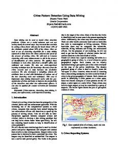
Classifier: ranking pattern candidates The Classifier module takes all the candidate design pattern instances identified by the Joiner and evaluates their similarity to the searched design pattern, to be able to rank them. Figure 7.1 shows an example of the classification process. This chapter introduces the approach, explains the motivation of the choices made during its design, the found solutions and the enhancements applied during its development and experimentation. Finally, the interaction of MARPLE-DPD with the user is described, reporting some example screenshots of the user interface.
7.1
Introduction to the learning approach
The rationale behind the approach is that the Joiner module finds all the instances matching an exact rule; this rule is written trying to keep it very general, so the matching tends to produce a large number of instances (having very high recall), but many of them are false positives (so the precision is low). However, the returned instances also carry a lot of information that the recognition rule does not use: all the micro-structures found in the classes belonging to the instances. A classifier has the possibility to choose the right instances among the ones extracted by the Joiner module, exploiting the micro-structures not used by the Joiner. Without the support of the Joiner, a simpler approach to the problem would be to submit every class, or worse, every possible group of classes of the system to the classification algorithm; such an approach would be very resource-demanding, and would require a lot of correct pattern instances to training the classifiers. The approach described here has the benefit of submitting a smaller number of candidates to the classifier, but with a higher percentage of true instances. In this way, the performance estimation is more accurate and the dataset contains a smaller quantity of noise, because it is focused only on a specific subset of the domain. The choice of using a classification process after an exact matching is one of the principal features characterizing the approach; the same rationale is used also, for example, by Ferenc et al. [69], while other authors tried the full-classification approach, e.g. Guéhéneuc et al. [90]. A discussion of machine learning approaches for design pattern detection can be found in Section 2.4. In some cases the same pattern can have different well known structural alternatives; these cases are handled in my approach in two ways: • If the different structural alternatives have the same set of roles, and they are organized in the same structure, the alternatives are handled by a single rule composed of the union of different constraints; for example, an Adapter design pattern is known in two major 79
Design Pattern Instance R1
R3
R2
Role Mappings Generator
Role Mapping 1 R1
R2
Role Mapping 1
R3
R1
R2
R3
CLUSTERER k
New Design Pattern Representation c1
...
ci
...
ck
CLASSIFIER
Correct
Figure 7.1: Classification process 80
Wrong
variants: object Adapter and class Adapter. The two variants are composed of the same roles, i.e. Target, Adaptee and Adapter, and with the same organization. So the two variants are handled in the same detection rule. • If the set of roles of the different alternatives are different, or organized in a different structure, the alternatives are handled like different design patterns, and computed independently. Alternatives of this kind are for example derived from different interpretations of the pattern or from some design decisions, e.g. to include or exclude the Client role from the pattern definition. The integrated handling of structurally different alternatives of a design pattern will be handled by at the user interface level, adding some modeling effort to track the different variants. This is out of the focus of the thesis and it is considered future work. Through the current approach, depicted in Figure 7.1, I generate every possible valid role mapping {(R1 , C1 ), (R2 , C2 ), . . . , (Rn , Cn )} for each pattern instance, where each Ci is the class that is supposed to play the role Ri inside the pattern. These mappings are all of a fixed size (one element for each pattern role) and each class has a fixed number of features, where the features are the micro-structures retrieved in the class. In this way each mapping can be represented as a vector of features whose length is given by (num_f eatures ú num_roles). These vectors are grouped by a clustering [47, 104] algorithm, producing k clusters; each pattern instance is represented as a k-long vector, having in each position i the absence/presence of the i-th mapping. Since we know that an instance is a design pattern (or not) directly from the training set, we can label each vector with the class attribute and use the resulting dataset for the training of a supervised classifier. The early version of the approach was published in an international workshop [10], and then published in an international journal [19] in 2011.
7.2
Motivation
The design of a machine learning oriented solution to a classification problem leads to the modeling of the input and output format of the algorithms to employ. The typical expectation of a learning algorithm is to receive a dataset as input, i.e. a list of vectors (a matrix) where each vector represents one of the subjects of the classification. The representation is achieved by the usage of features: the i-th cell of the vector represents the value of the i-th feature used to describe the subject. During the learning of a supervised classifier, a special feature is expected that represents the class value of the subject. The class is the target of the classification problem, i.e. in a design pattern detection problem it can be a boolean value telling if the subject (a pattern candidate) represents a correct pattern instance. Table 7.1 shows an example of an input dataset for a design pattern classification problem, composed of n features, from F1 to Fn , a Class attribute allowing two values (correct, incorrect) and representing two instances, named Instance 1 and Instance 2; the one represented in Table 7.1 is therefore the target format to make possible the exploitation of supervised classification algorithms. Table 7.1: Example of the typical input format of a supervised F1 F2 . . . Fi . . . Fn≠1 Fn Instance 1 ... ... Instance 2 ... ...
classification algorithm Class correct incorrect
A deeper look to the target format makes the modeling problem clear: how can we represent a pattern instance as a feature vector, knowing from Subsection 6.2.1 that a design pattern 81
instance is a group of classes, of unknown size, and organized in a tree structure? What kind of features can be exploited? In Chapter 5 the concept of micro-structure was introduced and a lot of micro-structures of different kinds were described. Micro-structures are employed by the Joiner module (explained in Chapter 6) for the extraction of pattern instances, because they provide a way of representing different aspect of analyzed system, by exposing different properties independently and with the same syntax. A single micro-structure can match different kinds of code pieces that share a certain characteristic, and they are not ambiguous. They are designed to abstract from the details of the code and expose more abstract concepts. Given their properties, it would be logical to use micro-structures as features into our dataset representation. Table 7.2: Example format of a dataset representing classes using micro-structures as features M S1 M S2 M S 3 M S 4 M S5 Class 1 1 1 1 0 0 Class 2 0 0 1 1 1 Class 3 0 1 0 1 1 The direct representation of classes in a dataset form using micro-structures as features would lead to a dataset like the one shown in Table 7.2. The dataset represents three classes, on the rows, described by five different values of micro-structures (from M S1 to M S5 ); each cell contains 1 if the micro-structure is present in the class, and 0 if not. It is clear that the representation is very far from the target representation needed. The major issue is that the number of classes in a design pattern instance is unknown. If this was not true, it would be possible to build a dataset representation made by the micro-structure values of the classes belonging to a pattern concatenated, leading to vectors whose length is determined by Nms · Ncl , where Nms is the number of micro-structures used as features, and Ncl is the fixed number of classes belonging to a pattern. Each row would contain all the information available regarding a pattern instance. Unfortunately, the number of classes in a design pattern definition is not fixed. But the number of roles is fixed. The number of roles is the only fixed decomposition given by the definition of a design pattern. Applying the last modeling hypotheses to roles, instead of classes, and exploiting the way the Joiner module works it is possible to create a representation of each role mapping detected by the Joiner. Recalling the example used in Chapter 6 to explain the detection process, and in particular Figure 7.2, which gives an overview of the merging process applied to role mappings to create pattern instances, we can see that many role mappings concur to the creation of a single pattern instance. Keeping track of the role mappings use to create a pattern instance it is possible to undo the process and producing all the mappings building the detected instance. Figure 7.3 depicts a more complex example of the generation of all the mappings that concurred to the building of an Abstract Factory pattern instance. The classes are represented by circles, whose names are built composing a prefix string representing the name role played by the class, and a numeric suffix representing the particular class. The meanings of the prefixes are: af æ Abstract Factory, ap æ Abstract Product, cf æ Concrete Factory, cp æ Concrete Product. The list of mappings is clearly made by fixed size elements, and each element is a class. Composing this kind of representation with the direct micro-structure representation of classes shown in Table 7.2 it is possible to achieve a new representation of mappings as dataset rows, shown in Table 7.3 as an example composing the previous ones. In the example the two mappings (the rows) are represented by fifteen features, created combining three roles (R1 , R2 , R3 ) with five micro-structures (from M S1 to M S5 ). Every single feature Ri M Sj tells if the j-th micro82
AT Abstr. Class
Mapping1
Mapping2
Merge
Match
IN Concr. Class
Instance1
Component Component
Composite
AT Component (Abstract Class) IN
IN
Composite (Concrete Class)
Leaf
Leaf (Concrete Class)
Figure 7.2: Merge process example (recalled). IN :Inheritance, AT : Abstract Type
af1 ap1
cf1 cp1
cf2
ap2 cp2
cp3
cp4
af1
cf1
ap1
cp1
af1
cf1
ap1
cp2
af1
cf1
ap2
cp3
af1
cf1
ap2
cp4
af1
cf1
ap2
cp5
af1
cf2
ap1
cp1
af1
cf2
ap1
cp2
af1
cf2
ap2
cp3
af1
cf2
ap2
cp4
af1
cf2
ap2
cp5
cp5
Figure 7.3: Mapping generation example for an Abstract Factory instance
83
structure is present in the class playing the i-th role in the respective mapping. Please notice that in this kind of dataset the information about pattern instances is lost: the rows represent the mappings, not the instances. There is no reference to the instance the mapping belongs to, and no class label; those pieces of information are kept out of the dataset and exploited in another moment. Summarizing, the dataset describes the classes contained in the mappings using only the micro-structures and the role assignments.
R1 M S2
R1 M S3
R1 M S4
R1 M S5
R 2 M S1
R2 M S2
R2 M S3
R2 M S4
R2 M S5
R3 M S1
R3 M S2
R 3 M S3
R3 M S4
R3 M S5
Mapping 1 Mapping 2
R1 M S1
Table 7.3: Example format of a dataset representing role mappings using micro-structures
1 0
1 1
1 1
0 1
0 0
0 0
1 0
1 1
1 0
0 0
1 1
1 0
0 1
1 1
1 0
A dataset having this format is not compatible with supervised classification, because each row is a role mapping, and not a pattern instance. Despite the incompatibility, the representation has the interesting property of being suitable as input for machine learning algorithms, while representing the information at a manageable abstraction level. In fact, the information about the belonging of a mapping to a pattern instance can be kept out of the dataset, and used in a different moment. For this reason a new elaboration step was added before the supervised classification in order to obtain only one feature vector for each instance. This step groups the mappings in clusters, and represents each pattern instance using the set of clusters its mappings belongs to. Figure 7.4 shows the follow-up of the previous example shown in Figure 7.1: The mappings are grouped by a clusterer algorithm in k = 10 clusters. Then the pattern instance is represented as a vector in a dataset, having k features (one for each cluster). Each cell of the vectors for the i-th feature tells if the instance (the row) contains a mapping that was clustered in cluster i. Adding the class label to the vector the target dataset form shown in Table 7.1 is obtained. The overall process handles the problem of the unknown size of the pattern instance imposing a number of clusters, therefore limiting the number of features to represent a single pattern instance to a fixed number. If the meaning of the dataset used for the clustering process is quite clear and directly related to the system and the pattern definition, the meaning of the last dataset is less obvious and requires a little discussion. The clustering process groups mappings, which can belong to different pattern instances, using the properties (described by micro-structures) of the classes they are composed of. No information about patterns is exploited. This means that the clusters represent a number of similar mappings, which we can call mapping types. An example can clarify the approach: a hypothetical clustering approach would be, for example, to create completely homogeneous clusters, i.e. where every element is identical to the others. A clustering approach like that would be feasible and could produce clusters containing more than one instance, because the representation of a class using micro-structure represents a projection of its structure in the micro-structure space, and there is no guarantee that the set of micro-structures employed in the experiments is able to uniquely identify a class in a system. Returning to the example, this particular clustering, applied to the generation of the second dataset, would produce a dataset where each feature represents one of the available combinations of {classes, roles, micro-structures} in the retrieved mappings. The example highlights two important problems. The first is that, as the number n of employed micro-structures grows, the number of possible combinations to represent a mapping grows exponentially, with the value of 2rn , where r is the number of roles of the pattern. The second problem is that the learning process is composed of 84
1
af1
cf1
ap1
cp1
10
af1
cf1
ap1
cp2
7
af1
cf1
ap2
cp3
af1
cf1
ap2
cp4
af1
cf1
ap2
cp5
af1
cf2
ap1
cp1
af1
cf2
ap1
cp2
af1
cf2
ap2
cp3
af1
cf2
ap2
cp4
10
af1
cf2
ap2
cp5
3
2
FALSE TRUE
3
4
5
6
7
3
C L U S T E R
2 5 2 3
k=10
8
9
2
10
TRUE FALSE TRUE FALSE TRUE FALSE FALSE TRUE
Figure 7.4: Cluster Generation
85
two steps: training and test, which correspond respectively to the moment when an algorithm learns about the domain, and creates its internal representation of it, and the moment in which new representations of the domain are evaluated. Given the learning process, a clustering algorithm like the one described in the example would not be able to handle new representations, different from the ones it already knows, and it would fail. For this reason a real clustering algorithm can be seen as a solution able to approximate that behaviour, having the advantage to be able to reasonably choose a cluster (in a fixed size set) for any new correctly encoded instance of the domain. The classification dataset is therefore an encoding of the input mappings, which uses information directly retrieved from the content of the system in the form of micro-structures. The encoding can always be created from a mapping because micro-structures are not ambiguous. Moreover, micro-structures are abstract features of the code, and role mappings are directly derived from the pattern definition and the analyzed system, so the dataset encoding maintains the semantics exposed by the two parts of the combination.
7.3
Evolution of the methodology
The classification methodology described up to now is a basic version. During the development and real implementation of the solution, many improvements were made to it. The remainder of this section describes the different improvements.
7.3.1
Micro-structures representation
The basic usage of micro-structures for the creation of the dataset of role mappings was to represent each micro-structure as a single boolean value telling if that micro-structure is present in that particular class. Micro-structures, as explained in Chapter 5, are binary relationships (or facts) among classes or other code entities. The fact of being unary is seen as a particular case where the source and destination of the micro-structure are the same. Some micro-structures are unary by definition, e.g. AbstractClass, FinalClass, Immutable: all the ones describing a simple property of a class. Being more precise with respect to the creation of the dataset (as explained up to now) every cell is a boolean value telling if a particular class in a role is the source of a particular micro-structure. This modeling loses the information about the destination of a micro-structure. An important property of micro-structures to remember is that, in general, there is no limit to the number of different micro-structures of the same kind contained in a class. For example, the Delegate EDP represents a method call existing between two methods belonging to different classes and with different signatures. It is clear that this kind of relationship is very common. To enhance the representation of the role mappings in the dataset, the information about the destination of each micro-structure was included: A new dimension was added to the definition of a single feature, representing the destination role of a particular micro-structure. Every feature is a boolean value defined as Ri M Sj Rk . A cell tells if in a mapping the class in the i-th role is the source of a micro-structure j having as destination the class in the k role of the same mapping. This representation better describes the mapping, fully exploiting the available information. Another improvement was done adding a default Other role to each mapping, representing every other class of the system (not represented by the current mapping), which is used as either source or destination (but not both of them) in the feature building described above. This solution allows the clusterer to have an approximated idea of the relationships among the represented mappings and the rest of the system. 86
7.3.2
Choice of the micro-structures
The improvement introduced in the previous subsection contributed to the creation of a plethora of features in the role mapping dataset representation. A deeper analysis of the available micro-structures resulted in a more accurate selection of the micro-structures to use. Table 7.4 contains the list of the micro-structures selected for the machine learning process, with additional simple properties added for the machine learning process. The content of Table 7.4 is called feature setup in MARPLE. The interpretation of the columns of the table is: Category: it is a categorization of the micro-structures: everything other than Micro Patterns and Elemental Design Patterns are Design Pattern Clues. Clues are divided in several categories, and some category is not present in the original catalogue. Cardinality: it admits two values (B: Binary, U: Unary). When it assumes the “Unary” value, the behaviour explained in Subsection 7.3.1 changes and reverts to the original one. In other words only one feature Ri M Sj Ri is produced for each role i and unary feature j. Del Self?: stands for “Delete self?”, and can be applied only to micro-structures having “Binary” cardinality. When “Del Self?” = “Yes”, the micro-structure will not produce a self link (where source is equal to destination). The consequence is that only features like Ri M Sj Rk , with i ”= k will be produced for micro-structure j having “Del Self?” = “Yes”.
Category
Name
Cardinality
Del Self?
Table 7.4: Micro-structures selection
Basic Attribute Information
OtherInstanceReference OtherStaticReference PrivateInstanceReference PrivateStaticReference ProtectedInstanceReference ProtectedStaticReference
B B B B B B
No No No No No No
Basic Class Relationship
AbstractMethodInvoked ClassInherited InterfaceInherited SameClass
B B B B
No Yes Yes Yes
Basic Method Information
ControlledParameter InheritanceThisParameter PrivateConstructor ProtectedConstructor
B B U U
No No
Basic Returned Elements Information
CloneReturned DifferentHierarchyObjectReturned SameHierarchyObjectReturned
U B B
Basic Type Information
FinalClass
U
Behavioural Clue
AbstractCycleTerminationCall
B
87
Yes Yes No
Category
Name
Behavioural Clue
AbstractCyclicCall ManyThisParameterCallTarget
B U
Elemental Design Pattern
AbstractInterface Conglomeration Delegate DelegatedConglomeration DelegateInFamily DelegateInLimitedFamily ExtendMethod Recursion Redirect RedirectInFamily RedirectInLimitedFamily RedirectRecursion Retrieve RevertMethod
U B B B B B B B B B B B B B
Information Clue
AbstractType CloneableImplemented ConcreteProductGetter ConcreteProductsReturned ControlledException ControlledInstantiation DirectReturnedObject EmptyConcreteProductGetter FactoryParameter MultipleReturnedObject MultipleReturns ReceivesParameter SingleReturnedObject VoidReturn
U U U U U B B U U B B B B U
AugmentedType Box Canopy CobolLike CommonState CompoundBox DataManager Designator Extender FunctionObject FunctionPointer
U U U U U U U U U U U
Micro Pattern
88
Del Self?
Cardinality
Table 7.4: Micro-structures selection
No
No Yes No Yes Yes Yes No Yes Yes Yes No No Yes
No No No No No No
Category
Name
Micro Pattern
Immutable Implementor Joiner Outline Overrider Pool PseudoClass PureType Record RestrictedCreation Sampler Sink Stateless StateMachine Taxonomy Trait
U U U U U U U U U U U U U U U U
Structural Clues
AdapterMethod AllMethodsInvoked ExtendedInheritance InstanceInAbstractReferred ProductReturns
U B B B B
Del Self?
Cardinality
Table 7.4: Micro-structures selection
No Yes No No
The feature setup is a more precise characterization of what is needed in the role mapping dataset, and contributes to a more compact and manageable feature space, without removing important information. The choice of the micro-structures was made by selecting the ones with a clear definition, removing the ones that were not completely proved and tested or that were not considered to be useful in a design pattern detection task. In fact, many other kinds of microstructures are available in MARPLE, e.g. for the detection of code smells and anti-patterns. In addition some new micro-structure was created, to better characterize some aspect of a software systems that were not addressed by the existing ones. The new micro-structures were designed to have some useful property when used as features. For example, the six “*Reference” micro-structures in the “Basic Attribute Information” category represent attributes of a class as links from the class to the type of the attribute. Their characterization is the combination of two criteria {Private, Protected, Other} and {Static, Instance} that characterize the modifiers of the attribute for visibility and the presence of absence of the static keyword. The characterization is total: each attribute can report only one of the six micro-structures. This kind of property allows to safely group the features by summarizing over one or both the criteria, reducing the number of features. The choice of grouping features can be done to enhance the machine learning performance for example when a set of features is too sparse to be significant or if the feature space is still to large to be computed. Grouping is only a planned feature, and it will be implemented in future work. The feature setup will be integrated with new information that will allow to automatically choose a set of features to group, e.g. when some programmable 89
constraints on the performance values and the feature space will be satisfied.
7.3.3
Single level patterns
The last important enhancement of the machine learning process is the handling of design patterns whose definitions are composed of only one level. Examples of this kind of patterns are Singleton and Adapter, whose merge rule diagrams are reported below. Singleton
T arget
Adapter
Adaptee
The problem with single-level patterns is that, applying the dataset generation process explained in this chapter to them, the output dataset, containing the representation of the instances using clusters as features, has a peculiar form. In fact, instances of design patterns with a single level are composed of only one mapping, producing a classifier dataset having only one true value per row. In fact, if each instance contains exactly one mapping, and the mappings are clustered in k clusters, each vector describing an instance will have k cells, one having value “true” (the one corresponding to the cluster containing the only mapping), and the other k ≠ 1 will have value “false”. A dataset in that form reduces the supervised classification problem to a choice of the best set of clusters representing the design pattern, which is an over-simplification, but a solution is available to improve this condition. In fact, if a single mapping is present in this kind of patterns, it is possible to directly use the role mapping dataset for the supervised classification, by adding the class label to each mapping, because there is only one of both for each instance. A slightly different approach was chosen, to avoid different implementations of similar processes: a bypass clusterer. When a single-level design pattern is analyzed, the applied clusterer simply produces a classifier dataset having the same number of features of the input dataset, using this criterion: cluster i contains a mapping if the value of the i-th feature of the mapping is “true”. In other words, it produces a copy of the input dataset, with different feature names. This solution allows the process to remain the same, adding only the choice of the right clusterer for the pattern. The only change to the methodology, is that the clustering phase shifts from a regular hard clustering task to a soft clustering [54, 149, 35] one. Soft clustering occurs when it is possible to assign an input vector to more than one cluster, creating a multi-categorization, like tagging on the web. Soft clustering is a generalization of the regular clustering, so the change in the methodology was simple and safe.
7.4
User experience
The MARPLE tool supports an iterative and incremental design pattern discovery and evaluation methodology. The user creates a “MARPLE Developer Project”, selecting which projects of the same workspace he wants to analyze. Then in the new project he creates a “MARPLE Developer File”, which is an xmi file containing the setup of the analysis. The editor shows a red box, representing the Information Detector. By right-clicking on the box and selecting “Run” from the menu the Information Detector starts and collects all the metrics and micro-structures contained in the analyzed project. Saving the analysis file triggers the save of all collected information. This behaviour is consistent for all the elaboration steps. Now MARPLE is ready for design pattern detection. By clicking “Add Elaboration Chain” in the Eclipse toolbar, two new boxes appear in the analysis editor, representing the Joiner (green) and the Classifier (blue) modules. A right-click on the outer yellow box lets to choose 90
the pattern to detect, by selecting the “Change chain properties” menu item. Once selected a pattern and confirmed, MARPLE is in a state like the one shown in Figure 7.5.
Figure 7.5: MARPLE configured for pattern detection The detection of design patterns candidates can be triggered by selecting the “Run” item in the contextual menu of the Joiner module. Then, selecting the “Show results” menu item a table view opens with the list of the detected design pattern candidates. For each pattern the names of the classes with role in the root level is shown, together with a combo box for the evaluation of the pattern and a column for the confidence value. Selecting a row and clicking the buttons “Graph” and “Joiner Model” in the “DP Instance Selection” view, two different graphical views of the selected pattern instance are shown, the first representing the classes as nodes in a graph (where the edges are the micro-structures), and the second following the graphical representation of the merge rule diagram (see Section 6.3). An example result is shown in Figure 7.6. After having inspected some instances, it is possible to evaluate them as “CORRECT” or “INCORRECT” using the combo box. After a number of instances have been evaluated, it is possible to submit them to the Classifier module. First, the “Copy instances to training” contextual menu item must be selected, and then the “Run training” one. The splitting of the two commands is caused by the fact that the instances used from the training are copied in a separate “training” project, which can be shared across many different analyses for different projects. The training project allows summing the instances coming from different systems to have a bigger training set. After the “Run training” command is finished, the clusterer and classifier algorithms have been trained and persisted to file, in the training project. At this point it is possible to select the “Run” menu item on the Classifier module, to fill the “Confidence” column in the “DP Instance Selection” view. An example of the evaluation of the Adapter design pattern is shown in Figure 7.7. 91
Figure 7.6: MARPLE showing a pattern candidate
Figure 7.7: MARPLE showing an evaluated pattern instance 92
7.5
Conclusion
This chapter described the machine learning methodology applied to the problem of design pattern detection. The methodology is focused on the modeling of the input and output formats of the learning algorithms employed. Machine learning algorithms traditionally work on datasets or matrices composed of vectors, which describe the domain of the problem. Domain modeling is important, sometimes crucial, in object-oriented software solutions: machine learning software solutions are not different in this sense. It is important to describe the domain to the algorithms in the best possible manner, to hope to have some kind of sensible results. Machine learning algorithms performances can be influenced by the input representation: Many techniques to improve their performance are based on the different kind of modification of the input format, like the use of kernel functions [166] in Support Vector Machines (SVM) [50] to change the feature space, or the selection of the features to use during the learning [88, 46, 48]. For this reason most of the effort was in the direction of dataset and feature modeling. Another important feature of the methodology is that it does not rely on a particular algorithm or set of algorithms, but it just focuses on the general formulation of supervised and unsupervised classification problem. No concrete technology or algorithm was mentioned in this chapter with the purpose of highlighting this aspect. The fact of being “algorithm-agnostic” brings a nice modularity in the implementation of the analysis system, allowing free plugging of different algorithms without the need of rewriting some kind of adaptation code.
93
94
Chapter 8
Experimentations with MARPLE-DPD The Classifier module was tested against the detection of five design patterns: Singleton, Adapter, Composite, Decorator, Factory Method. The detection rule for the five patterns are specified in Section 6.3, while the ones for all the other design patterns are available in Appendix A. This chapter explains the performed experiments and reports the obtained results.
8.1
Experiments
The experiments on the five design patterns were conducted applying a set of clustering and classification algorithms. The choice of the algorithms was made looking to the ones available for the Weka [196, 91] framework.
8.1.1
Algorithms
The choice of the algorithms to test resulted in the following list: • ZeroR is a simple classification rule that chooses always the dominant class; it is useful to include it in the tests because it provides a baseline telling how much the problem is unbalanced. • OneR [100] is a classification rule that chooses the attribute giving the minimum-error prediction for the classification. This is another kind of baseline useful to measure the difficulty of the problem. • NaiveBayes [109] is the simplest bayesian network available. It makes strong assumptions on the input: features are considered as independent. • JRip [49] is a rule learner. Its advantage is to be able to produce simple propositional logic rules for the classification, which are understandable to humans and simply translatable in logic programming. • RandomForest [41] is a classifier that build a forest of random decision trees, each one using a subset of the input features. • J48 [156] is an implementation of the C4.5 decision tree. It has the advantage of producing human-understandable rules for the classification of new instances. 95
• SMO [152, 113, 94] is an implementation of John Platt’s sequential minimal optimization algorithm for training a support vector classifier. In the experimentation only the RBF (Radial Basis Function) kernel is used in combination with this classifier. • LibSVM [63, 44] is another support vector machine (SVM) library, available to Weka using an external adapter. Two SVM variants are experimented (C-SVC, ‹-SVC), in combination with four different kernels (Linear, Polynomial, RBF, Sigmoid). • SimpleKMeans [23] is an implementation of the k means algorithm. It was exploited in two variants: with the Euclidean and Manhattan distances. • CLOPE [202] is a clustering algorithm for transactional data. Its advantages are being very fast and designed for nominal attributes datasets. • SelfOrganizingMap [120] is a clusterer that implements Kohonen’s Self-Organizing Map1 algorithm for unsupervised clustering. Self Organizing Maps are a special kind of competitive networks. • LVQ [121] is a clusterer that implements the Learning Vector Quantization algorithm for unsupervised clustering. • Cobweb [71, 75] is an hierarchical clusterer implementing the Cobweb and Classit clustering algorithms.
8.1.2
Projects
For each pattern, a set of pattern instances was extracted using the Joiner module, and then manually classified with the support of the user interface of the Classifier module, integrated with the Eclipse IDE. The set of projects used for the gathering of the design pattern instances was composed of a project containing example pattern instances gathered on the web, and the projects used for the PMARt [83] dataset. The summary of the experimented systems and some demographic metrics about them are shown in Table 8.1. Table 8.1: Projects for the experimentations Project
CUs
Packages
Types
Methods
DesignPatternExample 1 - QuickUML 2001 2 - Lexi v0.1.1 alpha 3 - JRefactory v2.6.24 4 - Netbeans v1.0.x 5 - JUnit v3.7 6 - JHotDraw v5.1 8 - MapperXML v1.9.7 10 - Nutch v0.4 11 - PMD v1.8
1060 156 24 569 2444 78 155 217 165 446
235 11 6 49 184 10 11 25 19 35
1749 230 100 578 6278 104 174 257 335 519
4710 1082 677 4883 28568 648 1316 2120 1854 3665
Attributes 1786 421 229 902 7611 138 331 691 1309 1463
TLOC 32313 9233 7101 79732 317542 4956 8876 14928 23579 41554
CUs: Number of Compilation Units — TLOC: Total number of Lines of Code 1
A more tested SOM package is available in MATLAB. Some tests were conducted with the MATLAB GUI, and a adaptation module was developed to call MATLAB from Java. Unfortunately, a non-documented incompatibility did not allow the Java-MATLAB bridge to work. It appears from the Mathworks support forum that it is not possible to train a neural network from Java.
96
Each Joiner rule was originally designed and tested against the project containing the example patterns. The idea behind the approach is to have the Joiner extracting (possibly) all the pattern instances contained in a software system, having virtually 100% recall. To achieve this goal, each rule (the ones in Chapter 6 and in Appendix A) was tuned to be able to catch all the pattern instances contained in the DesignPatternExampleproject. Then, the five rules of the experimented design patterns were enhanced during the experimentations. In fact, every pattern contained in the PMARt dataset was checked to be present in the results obtained by the Joiner, and when an instance was missed, the rule was analyzed and modified to include the missing instance (without losing the others). Another kind of enhancement was adding more selective constraints to avoid the explosion of the number of results. Some problems rose during the comparison with the PMARt dataset. The instances of the five tested patterns contained in PMARt revealed to be only partially correct. In particular, 14 instances out of 61; the 14 instances in PMARt contain 26 classes having key roles in their patterns, raising the number of wrong instances in the MARPLE definition to 26. The error contained in the dataset are of different kinds: for example in 4 - Netbeans v1.0.xorg .netbeans.modules.form.FormAdapter is reported as playing the Adapter role in the Adapter pattern, but it is an empty class; another example is net . sourceforge .pmd.ast.JavaParserConstants in 11 - PMD v1.8, which is reported as a Product for a Factory Method, but it is an interface only defining static constants, which has no meaning to instantiate. Other errors concerns, e.g., the wrong assignment of roles to some class in the pattern instance. The corrections will be discussed with the authors of PMARt after the submission if this thesis.
8.1.3
Patterns
The patterns to test were chosen by looking in the literature for the ones reported to be more frequent. The estimation was made analyzing the results coming from PMARt, the Design Pattern Detection Tool from Tsantalis et al. [194, 195] and design pattern detection results from Rasool et al. [157, 175]. Table 8.2 reports the amount of instances found and evaluated for each experimented pattern. The Adapter and Factory Method patterns have a number of candidates with a “+” suffix, because the number of candidates is not complete. In fact, those two patterns have been experimented only with the projects from “DesignPatternExample” to “4 - Netbeans v1.0.x”, because during the evaluation of instances in “4 - Netbeans v1.0.x”, in both cases, the number of evaluations grew over 1000, which I considered the threshold to decide to stop the manual evaluation. The decision of stopping to evaluate instances is motivated by the great amount of time employed in the evaluation task: the validation of a single pattern instance can take from 15 seconds to 5 minutes, depending on the complexity of instance itself. The 1000 threshold was set to reach a significant dataset for the patterns that made it possible. Table 8.2: Summary of detected pattern instances Pattern Singleton Adapter Composite Decorator Factory Method
Candidates
Evaluated
Correct
Incorrect
154 5861+ 128 250 2546+
154 1221 128 247 1044
58 618 30 93 562
96 603 98 154 482
The evaluations were then exploited for the search of the best classification setup. Singleton and Adapter are single-level patterns, so only classification algorithms were tested, while for the other patterns also clustering algorithms were included in the tests. 97
8.1.4
Parameter optimization
The search for the best parameter of a machine learning algorithm is a long, tedious, and error-prone (when results are recorded manually) task. Each algorithm has a set of parameters, each one having its domain, which can be of different types (i.e. continuous, discrete, boolean, nominal) and the entire set of parameters of a single algorithm is a potentially huge space to explore. The traditional way of exploring the space is a grid search2 , which means that every parameter must be discretized, by defining a discretization criterion for continuous parameters and assigning a discrete number to boolean and nominal ones. Then for each possible combination of parameters the algorithm must be tested and its performance values (e.g. confusion matrix, area under ROC, precision, recall) must be recorded. The set of performance values must be then analyzed and the best parameter set must be searched, defining one or more comparison criteria. The approach is defined to be sure to have a complete description of the parameter space with respect to the performance values. The problem with this methodology is that, as already introduced, it is time-consuming. A faster evaluation was needed, and an approach exploiting genetic algorithms was taken to try to reach the objective. Genetic algorithms [53, 127, 78] are an approach for the solution of optimization problems, inspired from the biological research and that allows sub-optimal solutions. Its general formulation is simple to adapt to different problems, and many implementation are available for research purposes. In particular I exploited JGAP3 , which is able to abstract from the algorithm details, providing a simple way of extending the framework just adding a new FitnessFunction . In general, optimization problems are characterized by the search for the best set of parameters to pass to a fitness function: when the maximum (or minimum for minimization problems) value is reached, the parameters are the optimal solution to the problem. The same kind of approach was already tested in the literature [163]. Performance estimators In my context, I defined a fitness function able to perform ten-fold cross validation[33, 178] over the evaluated pattern instances, using different performance indexes [26] as fitness values: accuracy, f-measure[197], area under ROC [40]. Accuracy Accuracy is one of the simplest performance measure for classification tasks: it is the percentage of correctly classified instances, in the positive and negative class. It is usually never reported alone, because it has several drawbacks, in particular when the positive and negative classes are unbalanced: a typical issue in classification tasks is having a little number of positive instances and a huge number of negative instances. In such cases, a naive classifier always giving the negative answers would have high accuracy. As the most important class is usually the positive one, it is clear that accuracy is not very useful as-is. Other kind of performance indicators exist. In fact, the second indicator employed is f-measure. F-measure It is defined (in the basic version) as the harmonic mean of precision and recall, which are other two performance values. Precision is the part of the positive-classified instances which is really positive, while recall is the part of really-positive instances classified as positive. The first measures the ability to correctly choose a positive instance, the second the ability to extract positive instances among the others. The two measures tend to be in contrast and the goal is usually to find the best trade-off value of the two. F-measure is a way of having a single number combining the two measures. 2 3
like suggested, e.g., in http://www.csie.ntu.edu.tw/~cjlin/papers/guide/guide.pdf http://jgap.sourceforge.net/
98
Area under ROC The last indicator is the area under ROC (Receiver Operating Characteristic). The ROC is a plot of true positive rate against false positive rate as the discrimination threshold of the classifier is varied. The area under ROC grows near to value 1 when the discrimination performs better, while bad classification brings values near to 0.5. The area under ROC has a stricter relation with the ability of ranking the results [67], because of the way the curve is built. All the described performance values are to be considered useful only in combination with each other and in relation to the domain. Moreover, research in machine learning and information retrieval is evolving, and some indicators are being criticized [92]. The approach taken in this experimentation is to rely on available performance indicators, exploiting the ones able to give a single score value and comparing the models from different perspectives.
8.2
Results
For each experimented design pattern, the classifiers’ setups having the best performance results are reported and discussed, together with the performance values. The experiments with the Classifier module are made on the output on the Joiner. Every direct or indirect performance value (including recall) is calculated on that particular dataset. In other words, the Classifier module performance is estimated under the hypothesis that the Joiner succeeded in extracting every pattern instance contained in the analyzed systems.
8.2.1
Singleton
Singleton is a single-level pattern, so only classifier algorithms were experimented. Table 8.3 reports the best results for each classifier type (the best value of the column is in bold font). When the same classifier is reported in different variants it is because some options lead to major differences in the algorithms being applied, e.g. the pruning setting in J48 and the SVM type and kernel in LibSVM. The numbers near the performance values are the identifiers of the configuration able to produce it; they will be used in Table 8.5 and Table 8.6 to uniquely identify a particular classifier setup. The values reported in Table 8.3 are the ones achieved during the parameter optimization procedure. The table shows performance values that can be considered quite good, because in many cases the values go beyond 0.9. The accuracy value near to 0.6 of the ZeroR classifier can be used as a simple measure of the balance between the classes, which is good because it is near to 0.5. At this level it is interesting to notice that the best performances were achieved by three different algorithm types. Table 8.4 gives a more detailed view of the distribution of the retrieved and evaluated instances among the different projects. The values are referred to the instances as they came from the Joiner, and how they were manually evaluated. No learning was involved in this phase. The classifier configurations whose performances are reported in Table 8.3 were then used to build an experiment in the Weka Experimenter module, which allows to test different classifiers against the same data and to compare their performance, calculating the standard deviations of the performance values and the statistical significance of the comparisons. In fact, to correctly compare different classifiers (with respect to one performance value), ranking the values is not enough, but a standard test must be applied with a significance value. The tests were conducted with the default 0.05 significance value. Table 8.5 contains the performance values, calculated using the Weka experimenter, for the classifiers defined in Table 8.3, accompanied by their standard deviations. For each classifier its reference number and class name are reported. The values are not the same (for the respective classifier setup) as the ones shown in Table 8.3, because the experimenter by default repeats each cross validation 10 times with different dataset 99
Table 8.3: Best performance results for the Singleton design pattern Classifier
accuracy
ZeroR OneR NaiveBayes JRip RandomForest J48 Unpruned J48 Reduced Error Pruning J48 Pruned SMO RBF C-SVC Linear C-SVC Polynomial C-SVC RBF C-SVC Sigmoid ‹-SVC Linear ‹-SVC Polynomial ‹-SVC RBF ‹-SVC Sigmoid
0.61 0.87 0.81 0.88 0.93 0.87 0.88 0.88 0.90 0.83 0.91 0.92 0.86 0.91 0.90 0.91 0.90
f-measure (1) (2) (3) (5) (7) (10) (13) (16) (19) (22) (25) (28) (31) (34) (37) (40) (43)
0.00 0.83 0.73 0.85 0.90 0.82 0.91 0.84 0.86 0.77 0.88 0.89 0.88 0.88 0.87 0.89 0.79
area under ROC (1) (2) (3) (6) (9) (12) (15) (18) (21) (24) (27) (30) (33) (36) (39) (42) (45)
0.48 0.86 0.89 0.88 0.97 0.91 0.85 0.91 0.94 0.87 0.94 0.95 0.94 0.93 0.94 0.95 0.92
(1) (2) (3) (4) (8) (11) (14) (17) (20) (23) (26) (29) (32) (35) (38) (41) (44)
Table 8.4: Singleton: evaluated instances summary Project DesignPatternExample 1 - QuickUML 2001 2 - Lexi v0.1.1 alpha 3 - JRefactory v2.6.24 4 - Netbeans v1.0.x 5 - JUnit v3.7 6 - JHotDraw v5.1 8 - MapperXML v1.9.7 10 - Nutch v0.4 11 - PMD v1.8 Total
Candidates
Evaluated
Correct
Incorrect
18 2 2 10 99 0 1 4 14 4
18 2 2 10 99 0 1 4 14 4
18 1 2 6 22 0 1 3 2 3
0 1 0 4 77 0 0 1 12 1
154
154
58
96
100
randomizations. The shown values are the average on the 10 different runs. To be able to tell which classifier is the best among the tested ones, and with a certain significance, it is possible to apply a ranking test in the Weka experimenter. Table 8.6 contains the ranking for the accuracy, f-measure and area under ROC of all the classifiers. The ranking test ranks the different classifiers by counting how many times each classifier significantly wins or loses against the other ones. The Wins≠Losses difference gives the ranking score, telling which classifier is the best. From the tables it is simple to understand that there is no single winner, but different algorithms perform best for different purposes. One of the most noticeable facts is that accuracy and f-measure give a similar ranking to the classifiers. In fact, classifiers (28), (41), and (42) occupy the top 3 positions. All the three classifiers are support vector machines using a RBF kernel, using LibSVM and two different SVM types. The top three positions for the area under ROC are given to the three RandomForest classifiers, instead, followed by another support vector machine with RBF kernel and from the (41) classifier. The overall results suggest that support vector machines with RBF kernel can be considered the best trade-off choice for the Singleton design pattern. The fact these good performance values are achieved on a relatively small dataset (less than two hundred instances) can be an indicator of the fact this pattern is simple to discriminate because the micro-structures are able to describe well its features, or that the dataset is biased in some way, and it would need more instances.
101
Table 8.5: Singleton: experiments summary. Significance level: 0.05 Classifier 1 2 3 4 5 6 7 8 9 10 11 12 13 14 15 16 17 18 19 20 21 22 23 24 25 26 27 28 29 30 31 32 33 34 35 36 37 38 39 40 41 42 43 44 45
accuracy
stddev
F-measure
stddev
auc
stddev
rules.ZeroR rules.OneR bayes.NaiveBayes rules.JRip rules.JRip rules.JRip trees.RandomForest trees.RandomForest trees.RandomForest trees.J48 trees.J48 trees.J48 trees.J48 trees.J48 trees.J48 trees.J48 trees.J48 trees.J48 functions.SMO functions.SMO functions.SMO functions.LibSVM functions.LibSVM functions.LibSVM functions.LibSVM functions.LibSVM functions.LibSVM functions.LibSVM functions.LibSVM functions.LibSVM functions.LibSVM functions.LibSVM functions.LibSVM functions.LibSVM functions.LibSVM functions.LibSVM functions.LibSVM functions.LibSVM functions.LibSVM functions.LibSVM functions.LibSVM functions.LibSVM functions.LibSVM functions.LibSVM functions.LibSVM
0.61 0.87 0.81 0.88 0.88 0.87 0.89 0.89 0.89 0.86 0.86 0.86 0.87 0.87 0.84 0.89 0.86 0.87 0.89 0.88 0.89 0.84 0.84 0.84 0.89 0.89 0.88 0.90 0.90 0.89 0.83 0.88 0.87 0.88 0.88 0.88 0.89 0.86 0.89 0.89 0.90 0.90 0.86 0.84 0.82
0.02 0.08 0.09 0.08 0.07 0.08 0.07 0.07 0.08 0.08 0.08 0.07 0.08 0.08 0.09 0.08 0.08 0.08 0.08 0.07 0.08 0.09 0.09 0.09 0.07 0.08 0.08 0.07 0.07 0.07 0.08 0.08 0.07 0.07 0.08 0.07 0.07 0.08 0.07 0.07 0.08 0.07 0.08 0.08 0.09
0.00 0.82 0.72 0.85 0.85 0.84 0.85 0.85 0.85 0.80 0.82 0.80 0.82 0.82 0.78 0.87 0.80 0.83 0.84 0.83 0.85 0.78 0.78 0.77 0.85 0.85 0.84 0.86 0.86 0.85 0.73 0.82 0.81 0.82 0.82 0.82 0.85 0.80 0.85 0.85 0.86 0.86 0.79 0.77 0.69
0.00 0.11 0.16 0.10 0.10 0.10 0.10 0.11 0.11 0.12 0.10 0.12 0.10 0.10 0.14 0.10 0.12 0.12 0.12 0.12 0.12 0.13 0.15 0.14 0.11 0.12 0.12 0.10 0.11 0.10 0.15 0.13 0.12 0.12 0.12 0.12 0.11 0.13 0.11 0.11 0.11 0.11 0.13 0.14 0.19
0.50 0.86 0.89 0.88 0.88 0.88 0.97 0.97 0.96 0.90 0.91 0.91 0.87 0.87 0.85 0.89 0.90 0.88 0.95 0.95 0.95 0.91 0.90 0.91 0.88 0.94 0.87 0.95 0.95 0.95 0.79 0.95 0.94 0.94 0.95 0.94 0.94 0.95 0.94 0.95 0.95 0.95 0.83 0.92 0.77
0.00 0.09 0.08 0.09 0.08 0.08 0.04 0.03 0.04 0.08 0.07 0.07 0.08 0.09 0.10 0.08 0.08 0.08 0.05 0.05 0.05 0.08 0.08 0.08 0.09 0.06 0.09 0.05 0.06 0.05 0.10 0.05 0.05 0.05 0.05 0.05 0.06 0.05 0.06 0.06 0.05 0.05 0.09 0.07 0.11
Average
0.87
0.80 102
0.90
Table 8.6: Singleton Classifier Ranking. W≠L: Wins≠Losses, W: Wins, L:Losses Accuracy Classifier W≠L (42) (28) (41) (40) (37) (29) (39) (30) (26) (25) (16) (8) (7) (21) (20) (19) (9) (36) (35) (43) (38) (34) (33) (32) (27) (18) (17) (14) (13) (12) (11) (10) (6) (5) (4) (2) (23) (24) (22) (15) (44) (31) (45) (3) (1)
9 6 5 5 5 5 4 4 4 4 4 4 4 3 3 3 3 2 2 1 1 1 1 1 1 1 1 1 1 1 1 1 1 1 1 1 0 -1 -1 -1 -4 -11 -16 -18 -44
W
L
9 6 5 5 5 5 4 4 4 4 4 4 4 3 3 3 3 2 2 1 1 1 1 1 1 1 1 1 1 1 1 1 1 1 1 1 1 1 1 1 1 1 1 1 0
0 0 0 0 0 0 0 0 0 0 0 0 0 0 0 0 0 0 0 0 0 0 0 0 0 0 0 0 0 0 0 0 0 0 0 0 1 2 2 2 5 12 17 19 44
f-measure Classifier W≠L (42) (41) (28) (30) (29) (25) (40) (16) (39) (37) (26) (21) (20) (19) (9) (8) (7) (6) (5) (4) (36) (35) (34) (27) (11) (38) (33) (32) (18) (14) (13) (2) (17) (12) (10) (23) (15) (43) (24) (44) (22) (31) (3) (45) (1)
8 8 8 6 6 6 5 5 4 4 4 4 4 4 4 4 4 4 4 4 3 3 3 3 3 2 2 2 2 2 2 2 1 1 1 0 0 -1 -3 -5 -5 -19 -24 -31 -44 103
W
L
8 8 8 6 6 6 5 5 4 4 4 4 4 4 4 4 4 4 4 4 3 3 3 3 3 2 2 2 2 2 2 2 1 1 1 1 1 1 1 1 1 1 1 1 0
0 0 0 0 0 0 0 0 0 0 0 0 0 0 0 0 0 0 0 0 0 0 0 0 0 0 0 0 0 0 0 0 0 0 0 1 1 2 4 6 6 20 25 32 44
area under ROC Classifier W≠L W (7) (9) (8) (21) (41) (19) (32) (30) (42) (40) (38) (36) (35) (34) (29) (28) (20) (39) (37) (26) (33) (11) (44) (12) (24) (22) (17) (10) (23) (16) (3) (27) (25) (18) (13) (6) (5) (4) (14) (15) (2) (43) (31) (45) (1)
25 24 24 20 19 19 17 17 16 16 16 16 16 16 16 16 16 14 14 14 13 3 1 1 0 0 0 0 -4 -14 -14 -18 -18 -18 -18 -18 -18 -18 -19 -21 -23 -28 -37 -39 -44
25 24 24 20 19 19 17 17 16 16 16 16 16 16 16 16 16 14 14 14 14 6 4 5 4 4 5 5 4 3 3 3 3 3 3 3 3 3 2 1 2 1 1 1 0
L 0 0 0 0 0 0 0 0 0 0 0 0 0 0 0 0 0 0 0 0 1 3 3 4 4 4 5 5 8 17 17 21 21 21 21 21 21 21 21 22 25 29 38 40 44
8.2.2
Adapter
The Adapter design pattern had the same experimental setup of Singleton. Table 8.7 contains the best results obtained during the parameter optimization, and it is interesting to see that the best performance were achieved always by support vector machines with a RBF kernel type, even if from two different kinds of algorithm. Table 8.7: Best performance results for the Adapter design pattern Classifier
accuracy
ZeroR OneR NaiveBayes JRip RandomForest J48 Unpruned J48 Reduced Error Pruning J48 Pruned SMO RBF C-SVC Linear C-SVC Polynomial C-SVC RBF C-SVC Sigmoid ‹-SVC Linear ‹-SVC Polynomial ‹-SVC RBF ‹-SVC Sigmoid
0.53 0.68 0.70 0.81 0.85 0.80 0.79 0.80 0.85 0.80 0.84 0.86 0.79 0.80 0.84 0.86 0.75
f-measure (1) (2) (3) (4) (7) (10) (13) (16) (19) (22) (25) (28) (31) (34) (37) (40) (43)
0.00 0.66 0.70 0.77 0.84 0.79 0.79 0.79 0.84 0.79 0.82 0.85 0.69 0.79 0.82 0.84 0.64
area under ROC (1) (2) (3) (5) (8) (11) (14) (17) (20) (23) (26) (29) (32) (35) (38) (41) (44)
0.50 0.68 0.78 0.82 0.92 0.86 0.84 0.86 0.92 0.85 0.89 0.92 0.84 0.85 0.91 0.93 0.82
(1) (2) (3) (6) (9) (12) (15) (18) (21) (24) (27) (30) (33) (36) (39) (42) (45)
The evaluation of the Adapter candidates stopped during the analysis of 4 - Netbeans v1.0.x, because the number of evaluated patterns reached 1221. Table 8.8 suggests that Adapter is widely present as a pattern, which is a confirmation for the considerations expressed in Section 6.3.2. Table 8.8: Adapter: evaluated instances summary Project DesignPatternExample 1 - QuickUML 2001 2 - Lexi v0.1.1 alpha 3 - JRefactory v2.6.24 4 - Netbeans v1.0.x 5 - JUnit v3.7 6 - JHotDraw v5.1 8 - MapperXML v1.9.7 10 - Nutch v0.4 11 - PMD v1.8 Total
Candidates
Evaluated
Correct
Incorrect
212 75 65 508 5003 -
212 69 65 500 375 -
128 13 44 261 172 -
84 56 21 239 203 -
5861+
1221
618
603
The usage of the Weka Experimenter of the best classifier configurations for the Adapter is 104
summarized in Table 8.9. The table shows data that are consistent with the ones shown for the Singleton pattern. In fact, the best-fitting classifiers are support vector machine and random forests. They are also among the ones with the lower standard deviation values. The overall shown performance is over 0.8 for the best setup, which can be considered good with respect to the 0.53 accuracy of ZeroR and ~0.65 performance of OneR. A deeper comparison of the classifiers is available in Table 8.10, which shows the ranking of the classifiers for the Adapter pattern. Classifiers number {(28),(29),(30),(40),(42)} are in the top five positions for all the three performance values. Even the difference in terms of Wins≠Losses is low (0 for the area under ROC). With no surprise, the classifiers are support vector machines with RBF kernels. RandomForest classifiers are lower in ranking, but the difference Wins≠Losses score is not much lower than the top positions. In fact, the first ten positions of the rank never lose a comparison, and the first 18 have a positive Wins≠Losses balance. The 18th position is the limit of significantly good classifiers. The classifiers in the first 18 positions are occupied by support vector machines and random forests. That 18th position line separates the classifiers that are significantly better than the others, and very distant in terms of ranking. The results for the Adapter and Singleton design patterns suggest that the classification strategy adopted for single-level design patterns is reasonable and produces sensible results. The performance values are high in both patterns and quite stable also when different randomizations of the dataset are used for the cross validation. In fact, the peak values shown in Table 8.7 are not much higher than the average values produced by the Experimenter and shown in Table 8.9, where the standard deviations are under 0.05 in most cases.
105
Table 8.9: Adapter: experiments summary. Significance level: 0.05 Classifier 1 2 3 4 5 6 7 8 9 10 11 12 13 14 15 16 17 18 19 20 21 22 23 24 25 26 27 28 29 30 31 32 33 34 35 36 37 38 39 40 41 42 43 44 45
accuracy
stddev
fmeasure
stddev
auc
stddev
rules.ZeroR rules.OneR bayes.NaiveBayes rules.JRip rules.JRip rules.JRip trees.RandomForest trees.RandomForest trees.RandomForest trees.J48 trees.J48 trees.J48 trees.J48 trees.J48 trees.J48 trees.J48 trees.J48 trees.J48 functions.SMO functions.SMO functions.SMO functions.LibSVM functions.LibSVM functions.LibSVM functions.LibSVM functions.LibSVM functions.LibSVM functions.LibSVM functions.LibSVM functions.LibSVM functions.LibSVM functions.LibSVM functions.LibSVM functions.LibSVM functions.LibSVM functions.LibSVM functions.LibSVM functions.LibSVM functions.LibSVM functions.LibSVM functions.LibSVM functions.LibSVM functions.LibSVM functions.LibSVM functions.LibSVM
0.53 0.68 0.70 0.77 0.77 0.77 0.83 0.83 0.83 0.77 0.76 0.77 0.76 0.76 0.75 0.76 0.77 0.76 0.83 0.83 0.82 0.78 0.78 0.78 0.82 0.82 0.81 0.84 0.84 0.84 0.77 0.63 0.76 0.78 0.78 0.77 0.82 0.82 0.82 0.84 0.83 0.84 0.67 0.47 0.74
0.00 0.04 0.04 0.04 0.04 0.04 0.04 0.04 0.04 0.04 0.05 0.04 0.05 0.05 0.05 0.05 0.04 0.05 0.04 0.04 0.04 0.04 0.04 0.04 0.04 0.04 0.04 0.04 0.04 0.04 0.04 0.05 0.04 0.04 0.04 0.04 0.04 0.04 0.04 0.04 0.04 0.04 0.14 0.00 0.04
0.00 0.65 0.70 0.73 0.73 0.73 0.82 0.82 0.82 0.75 0.75 0.75 0.75 0.75 0.73 0.74 0.75 0.75 0.83 0.82 0.82 0.76 0.76 0.77 0.81 0.81 0.80 0.83 0.83 0.83 0.75 0.67 0.74 0.77 0.77 0.75 0.81 0.81 0.81 0.83 0.82 0.83 0.63 0.64 0.72
0.00 0.05 0.05 0.05 0.05 0.05 0.04 0.04 0.04 0.05 0.05 0.05 0.05 0.05 0.06 0.05 0.05 0.05 0.04 0.04 0.04 0.05 0.05 0.05 0.04 0.04 0.04 0.04 0.04 0.04 0.05 0.04 0.05 0.04 0.05 0.04 0.04 0.04 0.04 0.04 0.04 0.04 0.16 0.00 0.05
0.50 0.68 0.78 0.76 0.76 0.76 0.91 0.92 0.92 0.78 0.81 0.83 0.81 0.81 0.80 0.80 0.80 0.83 0.91 0.83 0.91 0.77 0.78 0.83 0.88 0.88 0.88 0.91 0.91 0.91 0.83 0.71 0.83 0.78 0.78 0.84 0.89 0.82 0.89 0.91 0.83 0.91 0.66 0.50 0.80
0.00 0.04 0.05 0.04 0.04 0.04 0.03 0.03 0.03 0.05 0.05 0.04 0.05 0.05 0.05 0.05 0.05 0.04 0.03 0.04 0.03 0.04 0.04 0.04 0.03 0.03 0.03 0.03 0.03 0.03 0.04 0.05 0.04 0.04 0.04 0.04 0.03 0.04 0.03 0.03 0.04 0.03 0.14 0.00 0.05
Average
0.77
0.75 106
0.82
Table 8.10: Adapter Classifier Ranking. W≠L: Wins≠Losses, W: Wins, L:Losses Accuracy Classifier W≠L
W
L
(28) (40) (42) (30) (29) (41) (38) (37) (21) (20) (19) (9) (8) (7) (26) (25) (39) (27) (35) (34) (24) (36) (31) (23) (22) (33) (17) (12) (10) (6) (5) (4) (18) (16) (14) (13) (11) (15) (45) (43) (3) (2) (32) (1) (44)
31 29 28 28 28 27 27 27 27 27 27 27 27 27 27 27 27 27 8 8 8 7 7 7 7 6 6 6 6 6 6 6 5 5 5 5 5 5 5 2 3 3 2 1 0
0 0 0 0 0 0 0 0 0 0 0 0 0 0 1 1 2 5 18 18 18 18 18 18 18 18 18 18 18 18 18 18 18 18 18 18 18 21 26 31 39 39 41 43 44
31 29 28 28 28 27 27 27 27 27 27 27 27 27 26 26 25 22 -10 -10 -10 -11 -11 -11 -11 -12 -12 -12 -12 -12 -12 -12 -13 -13 -13 -13 -13 -16 -21 -29 -36 -36 -39 -42 -44
f-measure Classifier W≠L
W
L
(42) (29) (28) (30) (40) (41) (21) (20) (19) (37) (9) (8) (7) (39) (26) (25) (38) (27) (36) (35) (34) (33) (31) (24) (23) (22) (17) (18) (14) (13) (12) (11) (10) (16) (15) (6) (5) (4) (45) (3) (43) (32) (2) (44) (1)
32 32 32 31 30 28 28 28 28 27 27 27 27 27 27 27 27 27 7 7 7 7 7 7 7 7 7 6 6 6 6 6 6 5 4 4 4 4 4 3 1 2 1 1 0
0 0 0 0 0 0 0 0 0 0 0 0 0 4 4 4 5 9 18 18 18 18 18 18 18 18 18 18 18 18 18 18 18 18 18 18 18 18 27 34 33 39 40 41 44
32 32 32 31 30 28 28 28 28 27 27 27 27 23 23 23 22 18 -11 -11 -11 -11 -11 -11 -11 -11 -11 -12 -12 -12 -12 -12 -12 -13 -14 -14 -14 -14 -23 -31 -32 -37 -39 -40 -44 107
area under ROC Classifier W≠L W (42) (40) (30) (29) (28) (21) (19) (9) (8) (7) (39) (37) (26) (25) (27) (36) (31) (18) (12) (24) (41) (20) (38) (33) (14) (13) (11) (15) (45) (16) (17) (35) (34) (23) (22) (10) (3) (6) (5) (4) (32) (43) (2) (44) (1)
35 35 35 35 35 35 35 35 35 35 23 23 19 19 16 3 3 3 3 2 1 1 -1 -2 -7 -7 -7 -12 -15 -15 -17 -19 -19 -19 -19 -19 -19 -23 -23 -23 -37 -38 -39 -43 -43
35 35 35 35 35 35 35 35 35 35 33 33 31 31 30 18 18 18 18 17 16 16 14 15 8 8 8 5 8 5 5 5 5 5 5 5 5 5 5 5 3 2 2 0 0
L 0 0 0 0 0 0 0 0 0 0 10 10 12 12 14 15 15 15 15 15 15 15 15 17 15 15 15 17 23 20 22 24 24 24 24 24 24 28 28 28 40 40 41 43 43
8.2.3
Composite
The experimental setup for the Composite (and all the next patterns) is a bit different. First, Composite is a multi-level pattern, so it needs a clustering algorithm for the detection. Second, less clusterers and classifiers were employed for the experiments than the ones described in Subsection 8.1.1, making the experiments less time and resource-demanding. In Subsection 8.3.4 the issues related to clusterers are discussed. The reduction of the number of employed classifiers is given only by time constraints for the production of the results. Only the faster and better performing (on average) were kept. In particular all the LibSVM with kernels different from RBF were removed, and also the SMO classifier. The rationale is that, among the SVMs, the RBF is the kernel with better performance and lower computation time. SMO with the RBF kernel was removed because it performs similar to LibSVM with the RBF kernel. The best results achieved for the Composite design pattern are reported in Table 8.11. The performances are by far lower than the ones reported in Table 8.3 and Table 8.7 for the Singleton and Adapter design patterns, respectively. It is not possible to give an idea of the significance of the results, but some considerations can be formulated. First, the maximum (even if modest) performance values are scored by the support vector machines classifiers. Second, there is no clue for deducing which is the best clusterer among the two, even calculating the mean and standard deviation of the performance values for the two cases. Table 8.11: Best performance results for the Composite design pattern Clusterer
Classifier
accuracy
fmeasure
area under ROC
SimpleKMeans SimpleKMeans SimpleKMeans SimpleKMeans SimpleKMeans SimpleKMeans SimpleKMeans SimpleKMeans SimpleKMeans SimpleKMeans
ZeroR OneR NaiveBayes JRip RandomForest J48 Unpruned J48 Reduced Error Pruning J48 Pruned C-SVC RBF ‹-SVC RBF
0.75 0.75 0.77 0.75 0.75 0.75 0.77 0.75 0.79 0.81
(1) (2) (3) (4) (7) (10) (13) (16) (19) (22)
0.00 0.11 0.38 0.35 0.45 0.27 0.25 0.00 0.36 0.55
(1) (2) (3) (5) (8) (11) (14) (17) (20) (23)
0.39 0.50 0.63 0.48 0.61 0.59 0.51 0.51 0.88 0.67
(1) (2) (3) (6) (9) (12) (15) (18) (21) (24)
CLOPE CLOPE CLOPE CLOPE CLOPE CLOPE CLOPE CLOPE CLOPE CLOPE
ZeroR OneR NaiveBayes JRip RandomForest J48 Unpruned J48 Reduced Error Pruning J48 Pruned C-SVC RBF ‹-SVC RBF
0.75 0.75 0.75 0.81 0.81 0.81 0.81 0.75 0.81 0.77
(25) (26) (27) (28) (31) (34) (37) (40) (43) (46)
0.00 0.00 0.12 0.42 0.38 0.42 0.25 0.42 0.40 0.56
(25) (26) (27) (29) (32) (35) (38) (41) (44) (47)
0.39 0.50 0.52 0.60 0.65 0.53 0.56 0.58 0.61 0.72
(25) (26) (27) (30) (33) (36) (39) (42) (45) (48)
The summary of the per-project evaluated instance is available in Table 8.12. The table shows that all the available systems were analyzed, and their pattern candidates evaluated, because the total number of instances was less than 1000. In fact, only 128 instances were found 108
in all the systems analyzed. The not very high amount of pattern instances can be motivated by the diffusion of the pattern, which is high but not pervasive, and from the fact that Composite instances tend to be composed of many classes, and therefore of many role mappings. The size of the instances has the direct consequence of lowering the total number of the instances. Table 8.12: Composite: evaluated instances summary Project DesignPatternExample 1 - QuickUML 2001 2 - Lexi v0.1.1 alpha 3 - JRefactory v2.6.24 4 - Netbeans v1.0.x 5 - JUnit v3.7 6 - JHotDraw v5.1 8 - MapperXML v1.9.7 10 - Nutch v0.4 11 - PMD v1.8 Total
Candidates
Evaluated
Correct
Incorrect
27 5 1 2 71 1 5 5 10 1
27 5 1 2 71 1 5 5 10 1
15 1 0 0 9 1 2 0 2 0
12 4 1 2 62 0 3 5 8 1
128
128
30
98
One of the motivations of the low performances on this pattern could be the insufficient information contained in the dataset. Future work will try to demonstrate this hypothesis. The last major difference with the results of the first two design patterns is that no results are available from the Weka Experimenter: it is not possible to evaluate the significance level of the produced results. The reason is two-fold: • First, Weka is able to run only classification experiments (or other one-type only experiments), while the needed procedure is too complex. In fact, a single run requires the application of a clusterer chained with a classifier. Even writing a new classifier for Weka able to hide the complexity of the process to the Experimenter, a problem remains regarding the cross validation: the input of the clusterer is a dataset without the class labels, which is an information that stays outside the process until the supervised classification phase starts. Without the prior knowledge about the class labeling, the Experimenter is not able to record the analytical results for its estimations. • Second, even producing a dataset containing the summary data from all the experiments conducted during the optimization phase, the Experimenter is not prepared to handle all the produced data, and needs a huge amount of memory and time. In addition, the results would not be comparable, and the significance levels and standard deviations would have less meaning, because the data available from the optimization algorithm is the summary of an entire cross validation, while the Experimenter is designed to handle the results coming from all the single foldings of a cross validation, repeated a certain number of times on different randomizations of the same dataset. In Section 9.1 some future works related to these issues are described.
8.2.4
Decorator
The experiment regarding the Decorator design pattern has the same setup of the one on the Composite design pattern, for the same causes. 109
The best performance values obtained are shown in Table 8.13. The scenario is quite different from the one available in Table 8.11 for the Composite design pattern. The first significant difference is the splitting of the values between the two clusterers: SimpleKMeans beats CLOPE in most cases. Another difference is that the f-measure values for the Decorator are almost double of the ones in the Composite, and area under ROC values are significantly higher. At a first impression it seems that the Decorator dataset had a better classification outcome than the one for the Composite. One peculiarity of the results is that all the best performance values are scored by RandomForest classifiers. Random forests had good results also on the Singleton and Adapter patterns, but they never totally won over support vector machines. SVMs are just a bit lower in performance, and a suspect comes that, if a significance analysis was possible, the support vector machines could be considered equal or superior to the random forests, in the same way it happened for the first two patterns. Table 8.13: Best performance results for the Decorator design pattern Clusterer
Classifier
accuracy
fmeasure
area under ROC
SimpleKMeans SimpleKMeans SimpleKMeans SimpleKMeans SimpleKMeans SimpleKMeans SimpleKMeans SimpleKMeans SimpleKMeans SimpleKMeans
ZeroR OneR NaiveBayes JRip RandomForest J48 Unpruned J48 Reduced Error Pruning J48 Pruned C-SVC RBF ‹-SVC RBF
0.58 0.70 0.77 0.80 0.82 0.77 0.77 0.80 0.80 0.80
(1) (2) (3) (4) (7) (10) (13) (16) (19) (22)
0.00 0.56 0.74 0.76 0.77 0.75 0.73 0.76 0.75 0.76
(1) (2) (3) (5) (8) (11) (14) (17) (20) (23)
0.49 0.65 0.76 0.76 0.82 0.74 0.77 0.75 0.82 0.81
(1) (2) (3) (6) (9) (12) (15) (18) (21) (24)
CLOPE CLOPE CLOPE CLOPE CLOPE CLOPE CLOPE CLOPE CLOPE CLOPE
ZeroR OneR NaiveBayes JRip RandomForest J48 Unpruned J48 Reduced Error Pruning J48 Pruned C-SVC RBF ‹-SVC RBF
0.58 0.66 0.70 0.71 0.73 0.73 0.72 0.73 0.72 0.74
(25) (26) (27) (28) (31) (34) (37) (40) (43) (46)
0.00 0.59 0.67 0.65 0.72 0.66 0.68 0.65 0.66 0.70
(25) (26) (27) (29) (32) (35) (38) (41) (44) (47)
0.49 0.64 0.73 0.68 0.74 0.74 0.74 0.73 0.72 0.76
(25) (26) (27) (30) (33) (36) (39) (42) (45) (48)
The evaluated instances for the Decorator design pattern are more than the ones for the Composite, which are 128. In fact, the dataset is composed of 247 instances, 93 correct and 154 incorrect. The dataset is therefore also better balanced, having 38% of correct instances and 62% of incorrect instances, while the percentage for the Composite is respectively 23% and 77%. The better performance gained on the Decorator (with respect to the Composite) can be justified also with the larger size of the dataset, which is almost double, and the better balance between correct and incorrect instances that favours a better learning for the classifiers.
110
Table 8.14: Decorator: evaluated instances summary Project
Candidates
Evaluated
Correct
Incorrect
DesignPatternExample 1 - QuickUML 2001 2 - Lexi v0.1.1 alpha 3 - JRefactory v2.6.24 4 - Netbeans v1.0.x 5 - JUnit v3.7 6 - JHotDraw v5.1 8 - MapperXML v1.9.7 10 - Nutch v0.4 11 - PMD v1.8
31 16 6 12 131 7 14 16 11 6
31 16 6 12 128 7 14 16 11 6
10 2 0 1 59 1 5 8 6 1
21 14 6 11 69 6 9 8 5 5
Total
250
247
93
154
8.2.5
Factory Method
The last experimented pattern is the Factory Method, which has the same experimental setup of the last two analyzed patterns. In Table 8.15 the best results achieved for the Factory Method are reported. This results report another enhancement over the ones reported in Table 8.13 for the Decorator design pattern. The f-measure is over 0.8 in most cases, and the area under ROC reaches the maximum of 0.87. Accuracy values are comparable to the ones in for the Decorator, near to 0.8 in most cases. Another time, SimpleKMeans clearly beats CLOPE: results obtained through the CLOPE clusterer on the Factory Method are lower than the same experiments applied to the Decorator. There is a confirmation instead regarding the classifier algorithms: random forests have the maximum performance for all the indicators, and support vector machines are equal or a few behind. The real surprise in the table are the performances of NaiveBayes. In fact, while for all the other patterns it has an average or bad performance, here it scores performances very near to the top ones. The causes of these good scores are unknown, but some hypotheses can be formulated. The simplest one is that on this dataset the SimpleKMeans is able to group the mappings in a way that simplifies a lot the job of the classifiers, leading to good average results and the outstanding values of the NaiveBayes, which is a simple4 (but sometimes very effective) technique. A confirmation of this hypothesis is that, for example, for the Composite the NaiveBayes has performances comparable to the average ones, and very near to the ones of the ZeroR and OneR. These values suggest that the performed clustering did not help the classifiers to choose the correct instances. In the Decorator’s results, instead the values of ZeroR, OneR and NaiveBayes progressively grow, suggesting that as the complexity of the classifier augments, better results can be achieved because more complicated relationships among the features (the clusters) can be calculated. The best values are better than the ones for the NaiveBayes, but not so much. Finally, in the Factory Method there is the same performance growing, but the NaiveBayes has similar performances to the top ones. This last observation suggests that the extracted clusters are meaningful enough without, the need to combine their values in complicated ways, like more advanced classifiers are able to do. The number of instances found in the target systems for the Factory Method design pattern is huge compared with the Composite and Decorator patterns. One of the causes is the large 4
The naïve bayes classification technique is the simplest bayesian network. It is composed of one level, and assumes the input features are statistically independent, which is a strong assumption
111
Table 8.15: Best performance results for the Factory Method design pattern Clusterer
Classifier
accuracy
SimpleKMeans SimpleKMeans SimpleKMeans SimpleKMeans SimpleKMeans SimpleKMeans SimpleKMeans SimpleKMeans SimpleKMeans SimpleKMeans
ZeroR OneR NaiveBayes JRip RandomForest J48 Unpruned J48 Reduced Error Pruning J48 Pruned C-SVC RBF ‹-SVC RBF
0.52 0.70 0.81 0.76 0.82 0.80 0.78 0.79 0.82 0.80
(1) (2) (3) (4) (7) (10) (13) (16) (19) (22)
0.69 0.73 0.82 0.79 0.83 0.81 0.81 0.81 0.83 0.82
(1) (2) (3) (5) (8) (11) (14) (17) (20) (23)
0.50 0.70 0.87 0.77 0.87 0.86 0.85 0.85 0.84 0.87
(1) (2) (3) (6) (9) (12) (15) (18) (21) (24)
CLOPE CLOPE CLOPE CLOPE CLOPE CLOPE CLOPE CLOPE CLOPE CLOPE
ZeroR OneR NaiveBayes JRip RandomForest J48 Unpruned J48 Reduced Error Pruning J48 Pruned C-SVC RBF ‹-SVC RBF
0.52 0.54 0.55 0.54 0.55 0.55 0.55 0.55 0.56 0.56
(25) (26) (27) (28) (31) (34) (37) (40) (43) (46)
0.69 0.69 0.69 0.69 0.69 0.69 0.69 0.69 0.69 0.69
(25) (26) (27) (29) (32) (35) (38) (41) (44) (47)
0.50 0.53 0.55 0.52 0.57 0.54 0.55 0.54 0.54 0.58
(25) (26) (27) (30) (33) (36) (39) (42) (45) (48)
112
fmeasure
area under ROC
diffusion of this pattern, which simply prescribes an indirection in the responsibility of the creation of a new object, and another one is that the merge rule groups Factory Method instances using the Creator, ConcreteCreator and Product roles in the root level. The rationale is detailed in Section 6.3.1, and it is based on the definition and intent of the pattern itself. The sum of these causes led to 1044 pattern instances evaluated out of 2546 found ones. Also the balance is very good: 562 correct instances out of 482 wrong ones means that the 54% of the found instances were correct. Table 8.16: Factory Method: evaluated instances summary Project
Candidates
Evaluated
Correct
Incorrect
DesignPatternExample 1 - QuickUML 2001 2 - Lexi v0.1.1 alpha 3 - JRefactory v2.6.24 4 - Netbeans v1.0.x 5 - JUnit v3.7 6 - JHotDraw v5.1 8 - MapperXML v1.9.7 10 - Nutch v0.4 11 - PMD v1.8
269 55 18 159 2045 -
269 49 18 159 549 -
218 26 13 108 197 -
51 23 5 51 352 -
Total
2546
1044
562
482
As already outlined for the last two patterns, the size and composition of the dataset is important for the creation of the classification models. The one for the Factory Method is the larger dataset for the multi-level patterns and it is the better balanced, very near to the 1:1 ratio of correct and incorrect instances. This can be one of the causes of the performance values, which are better then the previous two ones.
8.3 8.3.1
Threats to validity and Limitations Design pattern definitions
The entire goal of this thesis is to provide a way of training the tool to understand what a pattern instance is and what is not. The machine learning approach was taken following the conjecture that it is not possible to formulate the precise formal definition of a pattern using only its implementation details, because the definition of a pattern is taught to designers through high level concepts and examples, and often designers learn patterns in different ways. This experiment was conducted by training classifiers using a labeling given from only one person, i.e. the author of this thesis. This condition influences (it must!) the results, in unknown directions. The interpretation of the results given in this chapter must be therefore interpreted in this sense “is this particular setup able to learn the definition of pattern x learned by this particular person?”. A better experiment would be to have training sets produced by different people, or better from an agreed and shared dataset, like the one we are trying to build through our DPB [15] project. The different personal interpretation of the design pattern definitions, in fact, reduces the reliability of the results of all the existing approaches in the literature, as every researcher defines the detection rules for design patterns following his interpretation of the definition. 113
8.3.2
Granularity
Currently the granularity of the micro-structures employed for the modeling of the analyzed system is at class level. This means that every micro-structure is recorded into the model as a link from a Type to another one or to itself. Micro-structures (represented by the BasicElement class into the model) are supported by the model as links from one CodeEntity to another one. CodeEntity is an abstract class representing every kind of clearly recognizable and referable piece of code, i.e. classes, attributes, methods, and also procedures and global variables (referring to non object-oriented code). The motivation of this choice is purely historical. MARPLE-DPD (see Chapter 4) is a project existing since 2008 and has been evolved to the current state. The module containing the Abstract Syntax Tree visitors catching the micro-structures was designed in order to support only class-level information granularity, while lower level granularity was supported using optional attributes. As the goal of this thesis is to demonstrate that data mining techniques applied to the pattern detection task are a sensible solution, the choice was to keep the existing (proved and tested) setup, and to focus on the development of the machine learning module. The consequence of the choice is that the current implementation is expected to have some kind of sub-optimal performances, especially regarding precision. In fact, placing information also at the method and attribute level could allow specifying detection rules able to express that the same method (having a role in the pattern) must satisfy a set of constraints, also related to some other role played by other classes/methods/attributes in the same pattern. The same applies to the Classifier module: more precise information can help the algorithm to have a precise description of the input, and to behave accordingly. I mentioned that this will impact on precision in particular, because the current implementation, specifying rules that must match patterns using more abstract information, must use less strict constraints, which statistically include more results and thus more correct pattern instances. The work for the immediate future will be to extend the approach to information placed to a more appropriate granularity level, in order to exploit all the information that can be extracted from the source code.
8.3.3
Libraries
The analysis of the connection from an analyzed system to its libraries is one of the major limitations of the approach. Most real-life software systems use lots of libraries to reach their goal. This is normal and it is what software reuse is about. The problem for design pattern detection is that many patterns are useful in order to extend frameworks (small or big) implemented into libraries. And frameworks use plenty of design patterns. The consequence is that in order to extract all the real instances of patterns existing in a system we should be able to represent an integrated model of the system and all its libraries. Unfortunately some issues arise, making the solution harder to implement. First, it is possible, especially in industry, that the source code of libraries is not available. Second, loading the model of every library connected to the system would mean handling a really huge model, whose significance would be low, as we expect a software system to use only a fraction of the classes of the libraries it relies on. The usage of such an integrated model like that would have many obvious performance consequences, in terms of both detection time and memory consumption. Even if the performance issues were solved, another modeling problem would raise: detecting patterns into a model including the analyzed system and all its libraries would extract also patterns which are exclusively contained in the libraries, which are of no interest to the user. Moreover a pattern half-implemented in a library is more related to the library, from the design point of view, than to the client system, but knowing about the connection between the two is useful information for program comprehension. The 114
ideal library handling, in the context of design pattern detection, would be to create a repository of single library analyzed models, which can be connected to the analyzed system model (like the libraries are connected to the system), and to exploit the joint information without the need to build the library model every time and already knowing the instances contained in the library. This kind of implementation needs a degree of design and scalability that is out of the scope of this thesis, but it is still the goal I think a reverse engineering tool should aim to. In the actual implementation, MARPLE does not handle the content of libraries, with the exception of inheritance, which is retrieved using the information provided by Eclipse using the compiler bindings. That kind of information is simple to retrieve and it is available also when the source code of the library is not available. Future work will aim to at least mitigate the issues coming from libraries and perhaps provide a degree of configuration of the desired behaviour.
8.3.4
Time and computational resources
The initial experimental setup was larger than the one reported in this chapter. In particular, more clustering algorithms were tested other than CLOPE and SimpleKMeans, i.e. SelfOrganizingMaps, LVQ, Cobweb. The achieved results are not reported because for different reasons those algorithms were not applicable. SelfOrganizingMap is too slow, at least one order of magnitude, compared to, e.g., SimpleKMeans. It takes 4 hours to learn the Composite dataset, for example. In addition, an undocumented problem does not allow the clusterer to handle nominal attribute, even if they are accepted without returning errors. The same applied for LVQ, which does not share the same computation time, however. In both cases the clustering is null (instances are all clustered in the same cluster) if the dataset is made by nominal attributes, and only a little better when nominal attributes are transformed to a numeric (0,1) form. Finally, Cobweb does not fit into memory for most of the inputs, even allocating 3500MB of Java heap. The remaining clustering algorithms, namely CLOPE and SimpleKMeans, are fast and have a small memory footprint, but they are also simpler as clustering technologies. For these reasons, newer and better results will be hopefully achieved by testing other clustering algorithm implementations, as outlined in Section 9.1.
8.4
Conclusion
This chapter described the experimental setup for the Classifier module, and the results obtained over five different design patterns. Despite the experienced difficulties, especially regarding the clustering algorithms, some overall considerations can be formulated. First, it seems that, in the average case, the kinds of classification algorithm having the best performance are the support vector machines, when paired with a RBF kernel. This is not a real surprise, as it is one of the most common kernels for SVMs and it is the default one, for example, in LibSVM. The second classifier was RandomForest, which is less stable in the performances, but reaches higher area under ROC values, better also than SVMs. Second, as the size of the dataset grows, the performance values increase also on multi-level patterns, and a difference between the SimpleKMeans and the CLOPE clusterers becomes more evident. In fact, in the results for the Decorator, and more in the ones for the Factory Method, the clustering performed by the SimpleKMeans produces datasets that are classified with better performances. A peculiarity of the last experiment, the one on the Factory Method pattern is that the NaiveBayes classifier, which is not as advanced as, e.g., as support vector machines, as performance values very near to the top ones, scored by RandomForest and LibSVM. It will be 115
interesting, in the future, to test new clustering algorithms and to augment the smaller datasets, to understand if better performances can be achieved. Another important validation of the approach is to compare its results with the results coming from other tools. A first attempt to provide this kind of validation is reported in Appendix C.
116
Chapter 9
Conclusions and Future Developments Many approaches have been developed by the research community for design pattern detection. This thesis described an approach that applies data mining techniques to the design pattern detection problem, to solve the issues related to the informal definition given to design patterns, which often leads to slightly different interpretations by different developers. The approach is implemented in the MARPLE tool, building the MARPLE-DPD module. MARPLE-DPD allows a user to detect patterns, exploiting existing rules or new ones, and to train some clusterer and classifier algorithms to learn what a good pattern instance is and what is not. The training consists of submitting to the algorithms a set of example pattern instances, which have been labeled as correct or incorrect, to let them build an internal model able to perform their evaluations. New pattern instances can then be automatically evaluated without having been inspected by the user. The automatic evaluation gives a confidence value to each pattern instance, which measures how much an instance is compliant with the set of examples submitted in the training phase. In this thesis the design pattern detection area has been analyzed from different perspectives. A review of the different approaches for design pattern detection highlighted that only few existing approaches try to overcome the limitations of exact matching techniques. By exploiting some kind of soft computing or machine learning techniques, which are designed to approximate the optimal solution of decision problems, it is possible to address the design pattern definition informality issue. The four reviewed approaches applying inexact matching exploit different techniques to solve the problem: machine learning, similarity scoring, and constraint relaxation. The machine learning approach most similar to the one described in this thesis is the one from Ferenc et al. [69], then extended by Fülöp [72]. In fact, it is the only approach using supervised classification to filter out wrong instances from a set of candidates. The apparent major limitation of that approach is that patterns are represented by features that mask their structure, while the approach introduced in this thesis employs lower level features, i.e. micro-structures. Similarity scoring does not involve the subjective view of the developer into the detection, while constraint relaxation is not able to learn from the choices made by the user when deciding to relax or not the rule. The other machine learning approach, which did not use exact matching for the extraction of patterns, was limited to represent one role at a time in the dataset, cutting the possibility to show the relationship among different the roles to the classifier algorithm. Given the requirements the usage of a classification as a filter is a better solution. The modeling aspect has a great relevance in reverse engineering, so a review of the available models for reverse engineering was performed. It turned out that, despite different good solutions are available, no one appears to be going to become a de facto standard. The only available 117
model for design pattern detection results, DPDX [117], was reported, discussed and compared to the model existing in MARPLE-DPD for the same purpose. DPDX has a different goal than the model employed in MARPLE-DPD. In fact, DPDX is wider and more complete, and is designed for the exchange of information among research groups, while the MARPLE-DPD model has the only goal of representing the structure of design pattern instances. One of the information available in DPDX and not in MARPLE-DPD, for example is the justification of the role assignments. Finally, DPDX lacks a meta-meta-model definition able to express the grammar of pattern definitions; this limitation can be problematic for users writing new pattern definitions and wanting to test the compliance of the definition with the model. One of the central points of the model integrated in MARPLE for the representation of an analyzed system is the concept of micro-structure. A micro-structure is a fact regarding one or two classes, having the property of being mechanically recognizable from the source code. This property makes micro-structures very useful for the abstraction of software systems. MARPLE supports three different families of micro-structures: elemental design patterns, micro patterns and design pattern clue. Each of these have been discussed and analyzed. Micro-structures are also the base for the pattern detection facilities in MARPLE-DPD. In fact, the Joiner module exploits micro-structures as edges in the graph it uses to represent the software system; the nodes are represented by the classes. Patterns are extracted by matching query rules against the graph, and then grouping the extracted role-class mappings in tree-wise structures representing pattern instances. The grouping (called “merge” in the Joiner) procedure is one of the most important parts of the entire approach, because it allows to define the roles identifying a pattern instance and their dependencies. The Joiner rules for all the design patterns of the GoF book have been defined, and the rules for the five design pattern which had the deeper experiments are discussed. In particular, many issues regarding the definition of the patterns are highlighted, and some proposals to overcome these issues are made. For example, the Adapter design pattern was found to be pervasive in software systems, when allowing all the possible interpretations available in the literature and in the analyzed system. A proposal for a different and formal interpretation of the Adapter design pattern has been then introduced, able to express the amount of adaptation performed by each class. The same rationale can be applied also to the Decorator and the other patterns defining an object indirection protocol. The rules defined for the Joiner were written and tested to maximize the number of detected patterns, admitting to retrieve many false positives. This criterion is based on the fact that the classification phase will filter out false positives, but it cannot extract correct instances from the system by itself. The Classifier module assumes the Joiner to have 100% recall. The classification approach was then described, and the modeling aspect of the supervised classification problem was discussed. The proposed solution is to split the process in two phases, the first exploiting clustering and the second supervised classification. The clustering phase transforms a dataset composed of the role-class mappings in a dataset representing the instances. The first dataset uses a combination of roles and micro-structures as features, while the second uses the information coming from the clustering phase to represent the pattern instances. The advantage of this approach is that it is able to represent pattern instances composed of an arbitrary number of classes as feature vectors of fixed size, which can be consumed by data mining algorithms. A major enhancement to the process is the special handling of patterns modeled with a single level. This kinds of pattern instances are composed of only one mapping. This property enables the direct usage of supervised classification on the first kind of dataset, allowing the classification algorithm to build its model on a representation that is more close to the system. The classification process was tested through a set of experiments on five design patterns: Singleton, Adapter, Composite, Decorator and Factory Method. The patterns were extracted 118
from a set of systems composed of the ones contained in the PMARt dataset plus one system containing example pattern instances. Many clustering and classification techniques, limiting to the ones having an implementation in the Weka framework, have been experimented on the five design patterns, with different results. More precisely, when clustering techniques are applied, the performance of the approach is lower than when applying only classification techniques. In the latter case, instead good performance values were achieved. The lower performances of the clustering process (than the direct classification one) can be caused by different factors. To have a confirmation of the performance degrade it will be necessary to be able to apply some of the clustering algorithms that were not runnable in the time limits, due to their implementation and to the limitations of computational resources. The best performances were obtained on the Singleton design pattern, which is a single-level pattern. The performances for the Adapter are only a little lower: Singleton scores ~0.9 of f-measure and ~1.0 of area under ROC, and Adapter ~0.8 and ~0.9, respectively, which are both good results. The best result on multi-level patterns is the one obtained on the Factory Method, which reached values similar to the ones of the Adapter, but ~0.05 lower. The performances for the Decorator are slightly lower and the ones for the Composite are not good. One of the outcomes of the experiments on these three patterns is that there is an apparent increase in the performances when the size of the dataset grows; moreover, as the dataset grows, also the difference between the two clusterer algorithms becomes relevant, with SimpleKMeans achieving better performances than CLOPE. The hypothesis of the correlation of the size of the dataset and the performances should be tested with the approach of learning curves [151]. Some problems raised through the manual evaluation and labeling of the results coming from the Joiner module. In particular, many of the instances reported in the PMARt dataset were not considered correct ones, and many others were not present in the dataset. If the second problem is normal in a manually validated dataset, the first one is more serious, tackling the validity of the dataset itself. Finally, the described approach demonstrated that an approach for the detection of design patterns exploiting data mining techniques can be successfully applied, despite the encountered technical limitations.
9.1
Future work
Many future works can be planned, and many were advised or described in the content of the thesis. Next paragraphs will summary a selection of the most relevant future developments. Micro-structures catalog The micro-structures catalog is not meant to be complete or perfect. Many new kinds of information can be specified, and others may be removed if they are not enough significant. A review of the catalog contents will be performed and new experiments will be done using the newer available information. Another task related to the catalog will be to test (empirically) the significance of the found micro-structures, in the same or similar way Gil and Maman did for micro patterns [76]. Micro-structures granularity The current implementation of the Micro Structure Detector reports micro-structures at the class level, i.e. information given by micro-structures is reported referring to classes. Some of this information should be reported at method or attribute level, leading to a more precise description of the underlying system. A more precise description will allow writing better Joiner rules, and it should imply better performances of the Classifier module. 119
Software architecture reconstruction integration MARPLE has architecture reconstruction facilities able to show graphs representing a software system, exploiting the micro-structures. As the model is enriched with the design pattern instances, the views will benefit from the integration of that information, which will augment the value of both the pattern detection and the architecture reconstruction modules. Design pattern instances pruning The pattern instances retrieved by the Joiner are modeled as trees of levels. The trees have the property of allowing the deletion of intermediate nodes without losing their correctness. The only limit is that, after the pruning, at least one class must play every role of the pattern. In future work, the user interface of MARPLE will allow the users delete levels from the pattern instances, permitting the cleaning of partially correct ones. Patterns interconnections Design patterns often exploited in combination with other ones. The representation of the connection among patterns will be useful to enhance the detection, and will have some application also in the SAR module: for example, when two patterns are connected and they have complementary goals, they can be shown as a single pattern or cluster of patterns. Variants or alternatives handling In some cases the same pattern has different structural alternatives, where the number and type of roles are not equal. If the different alternatives share the same intent, it will be possible to code the relationship in the pattern definitions, allowing the user interface to show the different alternatives under the same name, enhancing the user perception of the results. Libraries The handling of the connection among systems and libraries is one of the planned future works. The plan is to create an analysis repository for each library, and to recall it when a library is used by the analyzed system. The approach will permit to reuse existing analysis and to discover new usages of the patterns implemented in the libraries. New patterns One of the most obvious future works is to extend the experiments to all the other design pattern, which are reported in Appendix A. The new experiments will benefit from the experience gained with the experiments reported in this thesis, and errors due to algorithm implementations can be avoided. The results on all the patterns will allow better comparison with other results coming from different tools, exploiting for example the comparison functionalities of our Design Pattern Benchmark platform [15]. Clustering algorithm Given the results obtained through the clustering algorithms, one of the most important future developments is to test better clustering algorithm implementations, adapting them to the Weka interface if necessary. An interesting technique to try will be Self Organizing Maps1 . Dataset representation A new experiment to perform will be to represent also metrics in the datasets, and to represent micro-structures using their frequency values, absolute or relative, or to try more sophisticated frequency measures, like the TF-IDF [162] one. 1
The implementation used for the experimentations gave bad results. It needs more testing at least.
120
Feature grouping The current feature setup is not able to express the possibility of grouping different features to create more general ones. The grouping feature can be useful if the dataset representation that uses the basic features is too sparse, and can enhance both the time and results performances of the classification phase. Experimenter plugin The Weka Experimenter module is a great source of information about the significance of the performance values for classification algorithms. It allows to have a better informed view of the real reliability of the trained models and to sensibly rank different models. Unfortunately, only classification is supported as model scheme. A future work will be to provide a plugin for the Weka Experimenter to allow the evaluation of the full clusterer-classifier trained models, enabling the statistical analysis of the performances for the entire approach. One possibility will be to implement a meta-classifier that will mask the complete tool chain; another one will be to plug new weka.experiment. ResultListener or weka.experiment.ResultProducer classes to allow this functionality. If this kind of work will be too complicated, because it changes the way the Experimenter is designed, another possibility would be to modify the optimization algorithm to produce a fully-compliant Experimenter result file. During the experiments a partially compliant exporter was developed, but it produced too large and unmanageable files. Weka enhancement Many of the issues related to Weka during the experiments, especially in the Experimenter module, were related to observable design or implementation flaws in the code (which is open-source). Weka is becoming very popular in the research, and a contribution from the software engineering perspective could help to enhance a good initiative like it is, that brings data mining techniques to Java systems in a free and open manner. Full automation The effort in the last two points is in the direction of achieving full automation in the experiments, removing the issues related to the manual results collection. The only human-driven phases should be the evaluation of instances and the interpretation of the experimental results. Extensive comparison To better validate the approach, an extensive comparison with other tools, repositories and techniques will be performed, exploiting also the DPB [65] platform. The comparison will be performed against a number of system and instances that will make it statistically significant. A preliminary comparison against only one system is available in Appendix C.
121
122
Appendix A
Joiner rules for non-experimented patterns A.1 A.1.1
Creational Design Patterns Abstract Factory
Match rule The match rule for the Abstract Factory design pattern addresses only the basic concepts regarding the pattern definition. The constraints are related to the two hierarchies of factories and products, to the abstractness of AbstractFactory and AbstractProduct, and to the declarations of the returned products by the factories. Every other constraint will be tested by the classifier module, because Abstract Factory is a generic pattern allowing many different variants, like factory methods or prototypes as concrete factories. PREFIX BE :
SELECT ? A b s t r a c t F a c t o r y ? C o n c r e t e F a c t o r y ? A b s t r a c t P r o d u c t ? C o n c r e t e P r o d u c t WHERE { ? AbstractFactory BE : A b s t r a c t T y p e ? A b s t r a c t F a c t o r y ; BE : P r o d u c t R e t u r n s ? A b s t r a c t P r o d u c t . ? ConcreteFactory BE : E x t e n d e d I n h e r i t a n c e ? A b s t r a c t F a c t o r y ; BE : P r o d u c t R e t u r n s ? A b s t r a c t P r o d u c t . ? A b s t r a c t P r o d u c t BE : A b s t r a c t T y p e ? A b s t r a c t P r o d u c t . ? C o n c r e t e P r o d u c t BE : E x t e n d e d I n h e r i t a n c e ? A b s t r a c t P r o d u c t . NOT EXISTS {? A b s t r a c t F a c t o r y BE : S ame C lass ? A b s t r a c t P r o d u c t . } }
Merge rule The merge rule describes an Abstract Factory as an AbstractFactory class having some AbstractProducts and some ConreteFactory classes realizing it. Each AbstractProducts is realized by some ConcreteProduct.
< r o l e name=" A b s t r a c t F a c t o r y " /> < s u b l e v e l> < r o l e name=" C o n c r e t e F a c t o r y " /> < s u b l e v e l> < r o l e name=" A b s t r a c t P r o d u c t " /> < s u b l e v e l>
123
< r o l e name=" C o n c r e t e P r o d u c t " />
Merge rule diagram AbstractF actory AbstractP roduct ConcreteF actory ConcreteP roduct
A.1.2
Builder
Match rule The match rule for the Builder design pattern focuses on two elements Director and Builder must be linked my method calls, but they must be unrelated classes, and the ConcreteBuilder realizing the Builder must be able to return the Product. PREFIX BE :
SELECT ? D i r e c t o r ? B u i l d e r ? P r o d u c t ? C o n c r e t e B u i l d e r WHERE { {{? D i r e c t o r BE : D e l e g a t e ? B u i l d e r } UNION {? D i r e c t o r BE : R e d i r e c t ? B u i l d e r } UNION {? D i r e c t o r BE : D e l e g a t e I n L i m i t e d F a m i l y ? B u i l d e r } UNION {? D i r e c t o r BE : R e d i r e c t I n L i m i t e d F a m i l y ? B u i l d e r } } . ? ConcreteBuilder BE : E x t e n d e d I n h e r i t a n c e ? B u i l d e r ; BE : P r o d u c t R e t u r n s ? P r o d u c t . NOT NOT NOT NOT NOT NOT NOT NOT NOT NOT NOT }
EXISTS EXISTS EXISTS EXISTS EXISTS EXISTS EXISTS EXISTS EXISTS EXISTS EXISTS
{ { { { { { { { { { {
? D i r e c t o r BE : C r e a t e O b j e c t ? C o n c r e t e B u i l d e r . } ? D i r e c t o r BE : E x t e n d e d I n h e r i t a n c e ? B u i l d e r . } ? B u i l d e r BE : E x t e n d e d I n h e r i t a n c e ? D i r e c t o r . } ? B u i l d e r BE : Sam e Class ? D i r e c t o r . } ? P r o d u c t BE : E x t e n d e d I n h e r i t a n c e ? D i r e c t o r . } ? P r o d u c t BE : E x t e n d e d I n h e r i t a n c e ? C o n c r e t e B u i l d e r . } ? P r o d u c t BE : E x t e n d e d I n h e r i t a n c e ? B u i l d e r . } ? P r o d u c t BE : Same Class ? D i r e c t o r . } ? P r o d u c t BE : Same Class ? C o n c r e t e B u i l d e r . } ? P r o d u c t BE : Same Class ? B u i l d e r . } ? C o n c r e t e B u i l d e r BE : S t a t e l e s s ? C o n c r e t e B u i l d e r . }
Merge rule The merge rule tells that a Builder pattern instance is identified by its Director, which manages potentially more than one Builder. Each Builder is realized by some ConcreteBuilder, each one able to produce one Product kind.
< r o l e name=" D i r e c t o r " /> < s u b l e v e l>
124
< r o l e name=" B u i l d e r " /> < s u b l e v e l> < r o l e name=" P r o d u c t " /> < r o l e name=" C o n c r e t e B u i l d e r " />
Merge rule diagram Director Builder P roduct
A.1.3
ConcreteBuilder
Prototype
Match rule The match rule for the Prototype pattern specifies two main variants: classes creating instances of theirselves and returning them declared as a superclass, and classes that implement the java . lang . Cloneable interface, following the Java framework. PREFIX BE :
SELECT ? P r o t o t y p e ? C o n c r e t e P r o t o t y p e WHERE { {{? P r o t o t y p e BE : P r o d u c t R e t u r n s ? P r o t o t y p e . ? C o n c r e t e P r o t o t y p e BE : E x t e n d e d I n h e r i t a n c e ? P r o t o t y p e ; BE : C r e a t e O b j e c t ? C o n c r e t e P r o t o t y p e . { {? C o n c r e t e P r o t o t y p e BE : P r o d u c t R e t u r n s ? C o n c r e t e P r o t o t y p e . } UNION {? C o n c r e t e P r o t o t y p e BE : P r o d u c t R e t u r n s ? P r o t o t y p e } }. }UNION{ ? P r o t o t y p e BE : C l o n e a b l e I m p l e m e n t e d ? P r o t o t y p e . { {? C o n c r e t e P r o t o t y p e BE : E x t e n d e d I n h e r i t a n c e ? P r o t o t y p e . } UNION {? C o n c r e t e P r o t o t y p e BE : S a m e C lass ? P r o t o t y p e . OPTIONAL {? x BE : E x t e n d e d I n h e r i t a n c e ? P r o t o t y p e . } FILTER ( ! bound ( ? x ) ) } }. }}. }
Merge rule In the Prototype pattern there are only two roles, one child of the other. The ConcretePrototype is in a sublevel in order to group all the ConcretePrototypes for each Prototype.
< r o l e name=" P r o t o t y p e " />
125
< s u b l e v e l> < r o l e name=" C o n c r e t e P r o t o t y p e " />
Merge rule diagram P rototype ConcreteP rototype
A.2 A.2.1
Structural Design Patterns Bridge
The match rule for the Bridge design pattern looks for two separate hierarchies, connected through a reference from Abstraction or RefinedAbstraction to Implementor and wants the RefinedAbstraction to use the Implementor. PREFIX BE :
SELECT ? A b s t r a c t i o n ? I m p l e m e n t o r ? C o n c r e t e I m p l e m e n t o r ? R e f i n e d A b s t r a c t i o n WHERE { ? C o n c r e t e I m p l e m e n t o r BE : E x t e n d e d I n h e r i t a n c e ? I m p l e m e n t o r . ? C o n c r e t e I m p l e m e n t o r BE : O v e r r i d i n g M e t h o d " ? I m p l e m e n t o r . ? R e f i n e d A b s t r a c t i o n BE : E x t e n d e d I n h e r i t a n c e ? A b s t r a c t i o n . { {? A b s t r a c t i o n BE : O t h e r S t a t i c R e f e r e n c e ? I m p l e m e n t o r . } UNION{? A b s t r a c t i o n BE : P r i v a t e I n s t a n c e R e f e r e n c e ? I m p l e m e n t o r . } UNION{? A b s t r a c t i o n BE : P r i v a t e S t a t i c R e f e r e n c e ? I m p l e m e n t o r . } UNION{? A b s t r a c t i o n BE : O t h e r I n s t a n c e R e f e r e n c e ? I m p l e m e n t o r . } UNION{? A b s t r a c t i o n BE : P r o t e c t e d I n s t a n c e R e f e r e n c e ? I m p l e m e n t o r . } UNION{? A b s t r a c t i o n BE : P r o t e c t e d S t a t i c R e f e r e n c e ? I m p l e m e n t o r . } UNION{? R e f i n e d A b s t r a c t i o n BE : O t h e r S t a t i c R e f e r e n c e ? I m p l e m e n t o r . } UNION{? R e f i n e d A b s t r a c t i o n BE : P r i v a t e I n s t a n c e R e f e r e n c e ? I m p l e m e n t o r . } UNION{? R e f i n e d A b s t r a c t i o n BE : P r i v a t e S t a t i c R e f e r e n c e ? I m p l e m e n t o r . } UNION{? R e f i n e d A b s t r a c t i o n BE : O t h e r I n s t a n c e R e f e r e n c e ? I m p l e m e n t o r . } UNION{? R e f i n e d A b s t r a c t i o n BE : P r o t e c t e d I n s t a n c e R e f e r e n c e ? I m p l e m e n t o r . } UNION{? R e f i n e d A b s t r a c t i o n BE : P r o t e c t e d S t a t i c R e f e r e n c e ? I m p l e m e n t o r . } }. { {? R e f i n e d A b s t r a c t i o n BE : C o n g l o m e r a t i o n ? I m p l e m e n t o r . } UNION{? R e f i n e d A b s t r a c t i o n BE : D e l e g a t e ? I m p l e m e n t o r . } UNION{? R e f i n e d A b s t r a c t i o n BE : D e l e g a t e d C o n g l o m e r a t i o n ? I m p l e m e n t o r . } UNION{? R e f i n e d A b s t r a c t i o n BE : D e l e g a t e I n F a m i l y ? I m p l e m e n t o r . } UNION{? R e f i n e d A b s t r a c t i o n BE : D e l e g a t e I n L i m i t e d F a m i l y ? I m p l e m e n t o r . } UNION{? R e f i n e d A b s t r a c t i o n BE : ExtendMethod ? I m p l e m e n t o r . } UNION{? R e f i n e d A b s t r a c t i o n BE : R e c u r s i o n ? I m p l e m e n t o r . } UNION{? R e f i n e d A b s t r a c t i o n BE : R e d i r e c t ? I m p l e m e n t o r . }
126
UNION{? R e f i n e d A b s t r a c t i o n UNION{? R e f i n e d A b s t r a c t i o n UNION{? R e f i n e d A b s t r a c t i o n UNION{? R e f i n e d A b s t r a c t i o n }. NOT NOT NOT NOT NOT NOT NOT }
BE : R e d i r e c t I n F a m i l y ? I m p l e m e n t o r . } BE : R e d i r e c t I n L i m i t e d F a m i l y ? I m p l e m e n t o r . } BE : R e d i r e c t R e c u r s i o n ? I m p l e m e n t o r . } BE : RevertMethod ? I m p l e m e n t o r . }
EXISTS {? A b s t r a c t i o n BE : Sam e C l as s ? I m p l e m e n t o r . } EXISTS {? A b s t r a c t i o n BE : Sam e C l as s ? C o n c r e t e I m p l e m e n t o r . } EXISTS {? I m p l e m e n t o r BE : Sam e C l as s ? R e f i n e d A b s t r a c t i o n . } EXISTS {? C o n c r e t e I m p l e m e n t o r BE : Sam e C l as s ? R e f i n e d A b s t r a c t i o n . } EXISTS {? R e f i n e d A b s t r a c t i o n BE : E x t e n d e d I n h e r i t a n c e ? I m p l e m e n t o r . } EXISTS {? R e f i n e d A b s t r a c t i o n BE : Sam e C l as s ? I m p l e m e n t o r . } EXISTS {? R e f i n e d A b s t r a c t i o n BE : Sam e C l as s ? C o n c r e t e I m p l e m e n t o r . }
Merge rule The merge rule tells that the Bridge is identified by its Abstraction class, which manages a number of Implementors and has some realization as RefinedAbstraction. Each Implementor has some realization.
< r o l e name=" A b s t r a c t i o n " /> < s u b l e v e l> < r o l e name=" I m p l e m e n t o r " /> < s u b l e v e l> < r o l e name=" C o n c r e t e I m p l e m e n t o r " /> < s u b l e v e l> < r o l e name=" R e f i n e d A b s t r a c t i o n " />
Merge rule diagram Abstraction Implementor Ref inedAbstraction ConcreteImplementor
A.2.2
Facade
PREFIX BE :
SELECT ? Facade ? S u b s y s t e m C l a s s WHERE { {{ ? Facade BE : D e l e g a t e ? S u b s y s t e m C l a s s } UNION { ? Facade BE : R e d i r e c t ? S u b s y s t e m C l a s s } UNION { ? Facade BE : C o n g l o m e r a t i o n ? S u b s y s t e m C l a s s UNION { ? Facade BE : R e c u r s i o n ? S u b s y s t e m C l a s s }
127
}
UNION UNION UNION UNION UNION UNION UNION UNION
{ { { { { { { {
? Facade ? Facade ? Facade ? Facade ? Facade ? Facade ? Facade ? Facade
BE : RevertMethod ? S u b s y s t e m C l a s s } BE : ExtendMethod ? S u b s y s t e m C l a s s } BE : D e l e g a t e d C o n g l o m e r a t i o n ? S u b s y s t e m C l a s s BE : R e d i r e c t R e c u r s i o n ? S u b s y s t e m C l a s s } BE : D e l e g a t e I n F a m i l y ? S u b s y s t e m C l a s s } BE : R e d i r e c t I n F a m i l y ? S u b s y s t e m C l a s s } BE : D e l e g a t e I n L i m i t e d F a m i l y ? S u b s y s t e m C l a s s BE : R e d i r e c t I n L i m i t e d F a m i l y ? S u b s y s t e m C l a s s
}
} }}.
NOT EXISTS { ? Facade BE : E x t e n d e d I n h e r i t a n c e ? S u b s y s t e m C l a s s . } NOT EXISTS { ? S u b s y s t e m C l a s s BE : E x t e n d e d I n h e r i t a n c e ? Facade . } NOT NOT NOT NOT NOT NOT NOT NOT NOT NOT NOT NOT }
EXISTS EXISTS EXISTS EXISTS EXISTS EXISTS EXISTS EXISTS EXISTS EXISTS EXISTS EXISTS
{ { { { { { { { { { { {
? SubsystemClass ? SubsystemClass ? SubsystemClass ? SubsystemClass ? SubsystemClass ? SubsystemClass ? SubsystemClass ? SubsystemClass ? SubsystemClass ? SubsystemClass ? SubsystemClass ? SubsystemClass
BE : D e l e g a t e ? Facade . } BE : R e d i r e c t ? Facade . } BE : C o n g l o m e r a t i o n ? Facade . } BE : R e c u r s i o n ? Facade . } BE : RevertMethod ? Facade . } BE : ExtendMethod ? Facade . } BE : D e l e g a t e d C o n g l o m e r a t i o n ? Facade . } BE : R e d i r e c t R e c u r s i o n ? Facade . } BE : D e l e g a t e I n F a m i l y ? Facade . } BE : R e d i r e c t I n F a m i l y ? Facade . } BE : D e l e g a t e I n L i m i t e d F a m i l y ? Facade . } BE : R e d i r e c t I n L i m i t e d F a m i l y ? Facade . }
< r o l e name=" Facade " /> < s u b l e v e l> < r o l e name=" S u b s y s t e m C l a s s " />
Merge rule diagram F acade SubsystemClass
A.2.3
Flyweight
Complete rule The rule for the Flyweight pattern is completely specified using the XML syntax. Only little constraints are specified: the FlyweightFactory must create at least a ConcreteFlyweight instance and there must exist an inheritance of Flyweight and ConcreteFlyweight roles. Both the roles may not make method calls to FlyweightFactory, i.e. they cannot know about the existence of a factory managing them. The structure of the roles tells that the FlyweightFactory identifies the pattern, and it can manage many Flyweight types, which can be realized by many ConcreteFlyweight types. 128
< r o l e name=" F l y w e i g h t F a c t o r y "> < s u b l e v e l> < r o l e name=" F l y w e i g h t "> < s u b l e v e l> < r o l e name=" C o n c r e t e F l y w e i g h t ">
Merge rule diagram F lyweightF actory F lyweight ConcreteF lyweight
A.2.4
Proxy
The rule for the Proxy pattern is specified using the XML syntax. The rule defines the inheritance among Subject and {RealSubject, Proxy} roles. Proxy must keep a reference to the Subject or RealSubject and make a call to RealSubject. The pattern is identified by the Subject, which can be realized by many RealSubject and Proxy instances.
< r o l e name=" S u b j e c t "> < s u b l e v e l> < r o l e name=" R e a l S u b j e c t "> < s u b l e v e l> < r o l e name=" Proxy ">
129
Merge rule diagram Subject RealSubject
A.3 A.3.1
P roxy
Behavioral Design Patterns Chain of Responsibility
The rule for the Chain of Responsibility pattern is very simple. It defines the inheritance tree of Handler and ConcreteHandler and that the ConcreteHandler must make a call to the Handler, which must have at least an abstract method. The way the ConcreteHandler reaches the Handler is not defined. The structure of the pattern is simple: for each Handler, many ConcreteHandler may exist.
< r o l e name=" H a n d l e r "> < s u b l e v e l> < r o l e name=" C o n c r e t e H a n d l e r ">
Merge rule diagram Handler ConcreteHandler
A.3.2
Command
Match rule In the Command pattern the match rule cares about the ordering of the method calls among the roles, and the division between Commands (abstract and concrete) and the other roles. In fact, Commands may not extend Receivers or Invokers, and vice versa. In order to have a decent pattern implementation the Receiver must not call the ConcreteCommand, otherwise it means that the internal command layer is known to the implementation of the system. PREFIX BE :
SELECT ?Command ? R e c e i v e r ? ConcreteCommand ? I n v o k e r WHERE {
130
?Command BE : A b s t r a c t I n t e r f a c e ?Command . ? ConcreteCommand BE : E x t e n d e d I n h e r i t a n c e ?Command . ? I n v o k e r BE : A b s t r a c t M e t h o d I n v o k e d ?Command . { { ? ConcreteCommand BE : D e l e g a t e ? R e c e i v e r } UNION { ? ConcreteCommand BE : R e d i r e c t ? R e c e i v e r } UNION { ? ConcreteCommand BE : C o n g l o m e r a t i o n ? R e c e i v e r } UNION { ? ConcreteCommand BE : R e c u r s i o n ? R e c e i v e r } UNION { ? ConcreteCommand BE : RevertMethod ? R e c e i v e r } UNION { ? ConcreteCommand BE : ExtendMethod ? R e c e i v e r } UNION { ? ConcreteCommand BE : D e l e g a t e d C o n g l o m e r a t i o n ? R e c e i v e r UNION { ? ConcreteCommand BE : R e d i r e c t R e c u r s i o n ? R e c e i v e r } UNION { ? ConcreteCommand BE : D e l e g a t e I n F a m i l y ? R e c e i v e r } UNION { ? ConcreteCommand BE : R e d i r e c t I n F a m i l y ? R e c e i v e r } UNION { ? ConcreteCommand BE : D e l e g a t e I n L i m i t e d F a m i l y ? R e c e i v e r UNION { ? ConcreteCommand BE : R e d i r e c t I n L i m i t e d F a m i l y ? R e c e i v e r }. NOT EXISTS { ?Command BE : E x t e n d e d I n h e r i t a n c e ? R e c e i v e r . } NOT EXISTS { ?Command BE : E x t e n d e d I n h e r i t a n c e ? I n v o k e r . } NOT NOT NOT NOT NOT NOT NOT NOT NOT NOT NOT NOT
EXISTS EXISTS EXISTS EXISTS EXISTS EXISTS EXISTS EXISTS EXISTS EXISTS EXISTS EXISTS
{ { { { { { { { { { { {
? Receiver ? Receiver ? Receiver ? Receiver ? Receiver ? Receiver ? Receiver ? Receiver ? Receiver ? Receiver ? Receiver ? Receiver
NOT EXISTS { ? I n v o k e r NOT EXISTS { ? I n v o k e r }
}
} }
BE : D e l e g a t e ? ConcreteCommand . } BE : R e d i r e c t ? ConcreteCommand . } BE : C o n g l o m e r a t i o n ? ConcreteCommand . } BE : R e c u r s i o n ? ConcreteCommand . } BE : RevertMethod ? ConcreteCommand . } BE : ExtendMethod ? ConcreteCommand . } BE : D e l e g a t e d C o n g l o m e r a t i o n ? ConcreteCommand . } BE : R e d i r e c t R e c u r s i o n ? ConcreteCommand . } BE : D e l e g a t e I n F a m i l y ? ConcreteCommand . } BE : R e d i r e c t I n F a m i l y ? ConcreteCommand . } BE : D e l e g a t e I n L i m i t e d F a m i l y ? ConcreteCommand . } BE : R e d i r e c t I n L i m i t e d F a m i l y ? ConcreteCommand . } BE : E x t e n d e d I n h e r i t a n c e BE : E x t e n d e d I n h e r i t a n c e
?Command . } ? ConcreteCommand . }
Merge rule The Command pattern encapsulates actions into objects, exposing only a generic interface and permitting the choice of the real action to do at runtime. Of consequence, each Command may be used by many Invokers with many implementations (unknown to the invoker) that forward to specific Receivers.
< r o l e name="Command" /> < s u b l e v e l> < r o l e name=" R e c e i v e r " /> < r o l e name=" ConcreteCommand " /> < s u b l e v e l> < r o l e name=" I n v o k e r " />
Merge rule diagram 131
Command Receiver
A.3.3
ConcreteCommand
Invoker
Interpreter
The rule for the Interpreter design pattern defines first the inheritance tree of the expressions and forbids the Context to be in the same inheritance tree of the expressions. The expressions must receive the Context as a method parameter. The rule tells that there is one Context for each AbstractExpression, and many TerminalExpression and NonTerminalExpression for each AbstractExpression.
< r o l e name=" A b s t r a c t E x p r e s s i o n "> < r o l e name=" C o n t e x t "> < s u b l e v e l> < r o l e name=" T e r m i n a l E x p r e s s i o n "> < s u b l e v e l> < r o l e name=" N o n T e r m i n a l E x p r e s s i o n ">
Merge rule diagram
A.3.4
AbstractExpression
Context
T erminalExpression
N onT erminalExpression
Iterator
Match rule The match rule for the Iterator design pattern defines two inheritances of aggregators and iterators, which must be disconnected from one another, and looks for Iterators 132
which define all methods with no parameters (the StateMachine clause). The ConcreteIterator must call the ConcreteAggregate to get the next value or to test the stop condition. PREFIX BE :
SELECT ? I t e r a t o r ? A g g r e g a t e ? C o n c r e t e A g g r e g a t e ? C o n c r e t e I t e r a t o r WHERE { ? I t e r a t o r BE : S t a t e M a c h i n e ? I t e r a t o r . ? A g g r e g a t e BE : P r o d u c t R e t u r n s ? I t e r a t o r . ? C o n c r e t e A g g r e g a t e BE : E x t e n d e d I n h e r i t a n c e ? A g g r e g a t e . ? C o n c r e t e I t e r a t o r BE : E x t e n d e d I n h e r i t a n c e ? I t e r a t o r . {{? C o n c r e t e I t e r a t o r BE : C o n g l o m e r a t i o n ? C o n c r e t e A g g r e g a t e . } UNION{? C o n c r e t e I t e r a t o r BE : D e l e g a t e ? C o n c r e t e A g g r e g a t e . } UNION{? C o n c r e t e I t e r a t o r BE : D e l e g a t e I n F a m i l y ? C o n c r e t e A g g r e g a t e . } UNION{? C o n c r e t e I t e r a t o r BE : D e l e g a t e I n L i m i t e d F a m i l y ? C o n c r e t e A g g r e g a t e . } UNION{? C o n c r e t e I t e r a t o r BE : D e l e g a t e d C o n g l o m e r a t i o n ? C o n c r e t e A g g r e g a t e . } UNION{? C o n c r e t e I t e r a t o r BE : ExtendMethod ? C o n c r e t e A g g r e g a t e . } UNION{? C o n c r e t e I t e r a t o r BE : R e c u r s i o n ? C o n c r e t e A g g r e g a t e . } UNION{? C o n c r e t e I t e r a t o r BE : R e d i r e c t ? C o n c r e t e A g g r e g a t e . } UNION{? C o n c r e t e I t e r a t o r BE : R e d i r e c t I n F a m i l y ? C o n c r e t e A g g r e g a t e . } UNION{? C o n c r e t e I t e r a t o r BE : R e d i r e c t I n L i m i t e d F a m i l y ? C o n c r e t e A g g r e g a t e . } UNION{? C o n c r e t e I t e r a t o r BE : R e d i r e c t R e c u r s i o n ? C o n c r e t e A g g r e g a t e . } UNION{? C o n c r e t e I t e r a t o r BE : Re vertMethod ? C o n c r e t e A g g r e g a t e . } } . NOT EXISTS {? I t e r a t o r BE : E x t e n d e d I n h e r i t a n c e ? A g g r e g a t e . } . NOT EXISTS {? A g g r e g a t e BE : E x t e n d e d I n h e r i t a n c e ? I t e r a t o r . } . }
Merge rule The merge rule defines that an Iterator can manage different type of Aggregates, which can be realized by more than one ConcreteAggregate. Each Iterator can be realized by many ConcreteIterator types, not necessarily one for each ConcreteAggregate.
< r o l e name=" I t e r a t o r " /> < s u b l e v e l> < r o l e name=" A g g r e g a t e " /> < s u b l e v e l> < r o l e name=" C o n c r e t e A g g r e g a t e " /> < s u b l e v e l> < r o l e name=" C o n c r e t e I t e r a t o r " />
Merge rule diagram 133
Iterator Aggregate ConcreteIterator
ConcreteAggregate
A.3.5
Mediator
Complete rule The Mediator detection rule is defined using the XML syntax. Not many constraints are defined. Basically the inheritance trees of mediators and colleagues are defined, and the crossing calls among mediators and colleagues are required. The Mediator role identifies the pattern, which can manage many Colleague types. Mediator and Colleague types can be realized by many ConcreteMediator and ConcreteColleague ones.
< r o l e name=" M e d i a t o r "> < s u b l e v e l> < r o l e name=" C o l l e a g u e "> < s u b l e v e l> < r o l e name=" C o n c r e t e C o l l e a g u e "> < s u b l e v e l> < r o l e name=" C o n c r e t e M e d i a t o r ">
Merge rule diagram M ediator Colleague ConcreteM ediator
ConcreteColleague
A.3.6
Memento
Complete rule Memento is a pattern defined by a rule telling that Memento and Originator must by unrelated and that the Originator is a factory for the Memento, which is not Stateless and does not propagate calls to other classes. This is a single-level pattern; every instance is identified by the Memento-Originator pair. 134
< r o l e name=" Memento "> < r o l e name=" O r i g i n a t o r ">
Merge rule diagram M emento Originator
A.3.7
Observer
Match rule The match rule for the Observer pattern allows the abstract and concrete roles to collapse, while the Subject and Observer may not be covered by the same class. The other constraints specify that the ConcreteObserver makes the notification and that the Subject exposes a way to register the Observers. PREFIX BE :
SELECT ? S u b j e c t ? O b s e r v e r ? C o n c r e t e S u b j e c t ? C o n c r e t e O b s e r v e r WHERE { ? S u b j e c t BE : R e c e i v e s P a r a m e t e r ? O b s e r v e r . {{? C o n c r e t e O b s e r v e r BE : E x t e n d e d I n h e r i t a n c e ? O b s e r v e r . } UNION { ? C o n c r e t e O b s e r v e r BE : Sam e C lass ? O b s e r v e r . OPTIONAL { ? C o n c r e t e O b s e r v e r BE : E x t e n d e d I n h e r i t a n c e ? x . FILTER ( ? x != ? O b s e r v e r ) } FILTER ( ! bound ( ? x ) ) }} {{? C o n c r e t e S u b j e c t BE : E x t e n d e d I n h e r i t a n c e ? S u b j e c t . } UNION { ? C o n c r e t e S u b j e c t BE : Sam e C l as s ? S u b j e c t . OPTIONAL { ? x BE : R e c e i v e s P a r a m e t e r ? O b s e r v e r . ? C o n c r e t e S u b j e c t BE : E x t e n d e d I n h e r i t a n c e ? x . FILTER ( ? x != ? S u b j e c t ) } FILTER ( ! bound ( ? x ) ) }} { { ? C o n c r e t e S u b j e c t BE : D e l e g a t e ? O b s e r v e r } UNION { ? C o n c r e t e S u b j e c t BE : R e d i r e c t ? O b s e r v e r } UNION { ? C o n c r e t e S u b j e c t BE : C o n g l o m e r a t i o n ? O b s e r v e r } UNION { ? C o n c r e t e S u b j e c t BE : R e c u r s i o n ? O b s e r v e r } UNION { ? C o n c r e t e S u b j e c t BE : RevertMethod ? O b s e r v e r } UNION { ? C o n c r e t e S u b j e c t BE : ExtendMethod ? O b s e r v e r }
135
UNION UNION UNION UNION UNION UNION NOT NOT NOT NOT
{ { { { { {
? ConcreteSubject ? ConcreteSubject ? ConcreteSubject ? ConcreteSubject ? ConcreteSubject ? ConcreteSubject
EXISTS EXISTS EXISTS EXISTS
{ { { {
BE : D e l e g a t e d C o n g l o m e r a t i o n ? O b s e r v e r } BE : R e d i r e c t R e c u r s i o n ? O b s e r v e r } BE : D e l e g a t e I n F a m i l y ? O b s e r v e r } BE : R e d i r e c t I n F a m i l y ? O b s e r v e r } BE : D e l e g a t e I n L i m i t e d F a m i l y ? O b s e r v e r } BE : R e d i r e c t I n L i m i t e d F a m i l y ? O b s e r v e r }}
? S u b j e c t BE : E x t e n d e d I n h e r i t a n c e ? O b s e r v e r . } ? O b s e r v e r BE : E x t e n d e d I n h e r i t a n c e ? S u b j e c t . } ? S u b j e c t BE : Sam e Class ? O b s e r v e r . } ? C o n c r e t e O b s e r v e r BE : I n t e r f a c e ? C o n c r e t e O b s e r v e r . }}
Merge rule Each instance of the Observer pattern is identified by a couple of Subject and Observer roles. Each of them can have a concrete implementation.
< r o l e name=" S u b j e c t " /> < r o l e name=" O b s e r v e r " /> < s u b l e v e l> < r o l e name=" C o n c r e t e S u b j e c t " /> < s u b l e v e l> < r o l e name=" C o n c r e t e O b s e r v e r " />
Merge rule diagram
A.3.8
Subject
Observer
ConcreteSubject
ConcreteObserver
State
Match rule The match rule for the State pattern describes a Context class that may not be immutable and that calls methods belonging to a State class (which is not in its hierarchy), which is abstract and has at least one concrete implementation. PREFIX BE :
SELECT ? S t a t e ? C o n t e x t ? C o n c r e t e S t a t e WHERE { ? C o n c r e t e S t a t e BE : E x t e n d e d I n h e r i t a n c e ? S t a t e . {{ ? C o n t e x t BE : D e l e g a t e ? S t a t e } UNION { ? C o n t e x t BE : R e d i r e c t ? S t a t e } UNION { ? C o n t e x t BE : D e l e g a t e I n L i m i t e d F a m i l y UNION { ? C o n t e x t BE : R e d i r e c t I n L i m i t e d F a m i l y
? State } ? S t a t e }}
OPTIONAL {? x BE : C r e a t e O b j e c t ? S t a t e . } FILTER ( ! bound ( ? x ) ) NOT EXISTS { ? C o n t e x t NOT EXISTS { ? C o n t e x t
BE : E x t e n d e d I n h e r i t a n c e ? S t a t e . } BE : Immutable ? C o n t e x t . }
136
}
Merge rule One State pattern instance is identified by a State class and its Context. There can be many concrete implementations of the State.
< r o l e name=" S t a t e " /> < r o l e name=" C o n t e x t " /> < s u b l e v e l> < r o l e name=" C o n c r e t e S t a t e ">
Merge rule diagram State
Context
ConcreteState
A.3.9
Strategy
The Strategy pattern is a very general one. Its detection rule is very similar to the one of the State pattern, but many other patterns can be seen as specializations of Strategy: Builder and Factory Method, for example define two different way of implementing a strategy for object instantiation, and Visitor defines a strategy for handling different kind of elements of a data structure. Match rule In the match rule the Strategy pattern is defined as an inheritance of strategies, whose abstract class is used by a Context. The Context must keep a reference to the Strategy or receive it as a parameter, and it has to call it. PREFIX BE :
SELECT ? S t r a t e g y ? C o n t e x t ? C o n c r e t e S t r a t e g y WHERE { ? C o n c r e t e S t r a t e g y BE : E x t e n d e d I n h e r i t a n c e ? S t r a t e g y . {{ ? C o n t e x t BE : R e c e i v e s P a r a m e t e r ? S t r a t e g y } UNION { ? C o n t e x t BE : P r i v a t e I n s t a n c e R e f e r e n c e ? S t r a t e g y } UNION { ? C o n t e x t BE : P r o t e c t e d I n s t a n c e R e f e r e n c e ? S t r a t e g y }} {{ ? C o n t e x t BE : D e l e g a t e ? S t r a t e g y } UNION { ? C o n t e x t BE : R e d i r e c t ? S t r a t e g y } UNION { ? C o n t e x t BE : D e l e g a t e I n L i m i t e d F a m i l y UNION { ? C o n t e x t BE : R e d i r e c t I n L i m i t e d F a m i l y
? Strategy } ? S t r a t e g y }}
OPTIONAL {? x BE : C r e a t e O b j e c t ? S t r a t e g y . } FILTER ( ! bound ( ? x ) ) NOT EXISTS { ? C o n t e x t
BE : E x t e n d e d I n h e r i t a n c e
137
? Strategy .}
NOT NOT NOT NOT NOT NOT NOT NOT NOT NOT NOT NOT }
EXISTS EXISTS EXISTS EXISTS EXISTS EXISTS EXISTS EXISTS EXISTS EXISTS EXISTS EXISTS
{ { { { { { { { { { { {
? Strategy ? Strategy ? Strategy ? Strategy ? Strategy ? Strategy ? Strategy ? Strategy ? Strategy ? Strategy ? Strategy ? Strategy
BE : D e l e g a t e ? C o n c r e t e S t r a t e g y } BE : R e d i r e c t ? C o n c r e t e S t r a t e g y } BE : C o n g l o m e r a t i o n ? C o n c r e t e S t r a t e g y } BE : R e c u r s i o n ? C o n c r e t e S t r a t e g y } BE : RevertMethod ? C o n c r e t e S t r a t e g y } BE : ExtendMethod ? C o n c r e t e S t r a t e g y } BE : D e l e g a t e d C o n g l o m e r a t i o n ? C o n c r e t e S t r a t e g y } BE : R e d i r e c t R e c u r s i o n ? C o n c r e t e S t r a t e g y } BE : D e l e g a t e I n F a m i l y ? C o n c r e t e S t r a t e g y } BE : R e d i r e c t I n F a m i l y ? C o n c r e t e S t r a t e g y } BE : D e l e g a t e I n L i m i t e d F a m i l y ? C o n c r e t e S t r a t e g y } BE : R e d i r e c t I n L i m i t e d F a m i l y ? C o n c r e t e S t r a t e g y }
Merge rule The merge rule for the Strategy pattern is basically the same as the one for the State pattern. Each pattern instance is identified by a couple {Strategy, Context}; many Concrete Strategy instances are allowed for each pattern instance.
< r o l e name=" S t r a t e g y " /> < r o l e name=" C o n t e x t " /> < s u b l e v e l> < r o l e name=" C o n c r e t e S t r a t e g y " />
Merge rule diagram Strategy
Context
ConcreteStrategy
A.3.10
Template Method
Complete rule The Template Method pattern is detected using a rule that needs no more expressiveness than the XML syntax can provide. It is a very simple rule that specifies classes declaring an abstract method and calling it, and their subclasses. It is possible to have many Concrete Classes for each AbstractClass.
< r o l e name=" A b s t r a c t C l a s s "> < s u b l e v e l> < r o l e name=" C o n c r e t e C l a s s ">
138
Merge rule diagram AbstractClass ConcreteClass
A.3.11
Visitor
Match rule In the Visitor pattern the match rule defines the two inheritances and their relations. ConcreteElements pass theirselves to the Visitors and Visitors accept Elements as paramters. The abstract and concrete roles are allowed to collapse, but at least the two abstract roles must not be related one to the other. In addition, Concrete Visitors must have an implementation. PREFIX BE :
SELECT ? V i s i t o r ? E l e m e nt ? C o n c r e t e V i s i t o r ? C o n c r e t e E l e m e n t WHERE { ? V i s i t o r BE : I n h e r i t a n c e T h i s P a r a m e t e r ? C o n c r e t e E l e m e n t . ? E l e m e n t BE : R e c e i v e s P a r a m e t e r ? V i s i t o r . {{? C o n c r e t e E l e m e n t BE : E x t e n d e d I n h e r i t a n c e ? E l e m e n t . } UNION { ? C o n c r e t e E l e m e n t BE : Sam e C lass ? E l e m e n t . } } {{? C o n c r e t e V i s i t o r BE : E x t e n d e d I n h e r i t a n c e ? V i s i t o r . } UNION { ? C o n c r e t e V i s i t o r BE : Sam e C lass ? V i s i t o r . }} NOT NOT NOT NOT NOT
EXISTS EXISTS EXISTS EXISTS EXISTS
{ { { { {
? V i s i t o r BE : E x t e n d e d I n h e r i t a n c e ? E le m e n t . } ? E l e m e n t BE : E x t e n d e d I n h e r i t a n c e ? V i s i t o r . } ? V i s i t o r BE : Sam eC lass ? E le m e n t . } ? C o n c r e t e V i s i t o r BE : I n t e r f a c e ? C o n c r e t e V i s i t o r . } ? C o n c r e t e V i s i t o r BE : P s e u d o C l a s s ? C o n c r e t e V i s i t o r . }
OPTIONAL { ? C o n c r e t e E l e m e n t BE : Sam e C l as s ? E l e m e n t ; BE : E x t e n d e d I n h e r i t a n c e ? e . ? e BE : R e c e i v e s P a r a m e t e r ? V i s i t o r . } FILTER ( ! bound ( ? e ) | | ? e = ? Ele me n t ) OPTIONAL { ? C o n c r e t e V i s i t o r BE : Sam e C l as s ? V i s i t o r ; BE : E x t e n d e d I n h e r i t a n c e ? v . ? v BE : I n h e r i t a n c e T h i s P a r a m e t e r ? C o n c r e t e E l e m e n t . } FILTER ( ! bound ( ? v ) | | ? v = ? V i s i t o r ) OPTIONAL { ? C o n c r e t e V i s i t o r BE : Sam e C l as s ? V i s i t o r . ? cv BE : E x t e n d e d I n h e r i t a n c e ? V i s i t o r . } FILTER ( ! bound ( ? cv ) | | ? cv = ? C o n c r e t e V i s i t o r ) }
139
Merge rule A Visitor pattern instance is defined by a Visitor and its related Element. Their concrete implementations are each one if a different sublevel.
< r o l e name=" V i s i t o r " /> < r o l e name=" E le m e nt " /> < s u b l e v e l> < r o l e name=" C o n c r e t e V i s i t o r " /> < s u b l e v e l> < r o l e name=" C o n c r e t e E l e m e n t " />
Merge rule diagram V isitor
Element
ConcreteV isitor
ConcreteElement
140
Appendix B
Setup parameters for the experimented algorithms This appendix contains the setup of the parameters for each experiment reported in Chapter 8. The parameter names are taken from the parameters of the respective algorithm implementations found in Weka. When an algorithm has a major variant it was considered as a different algorithm. The name of the variant should be sufficient to setup the respective algorithm using the dedicated parameters, which are not reported here for brevity.
B.1
Setup of the genetic algorithm parameters
This section contains the list of the parameters exploited by the genetic algorithm for their optimization. For each parameter the range of tested values is reported. Boolean values have no range. When a boolean value has literals in the range cell, it means it was employed as a selector for a nominal parameter. The parameters are reported in Tables B.1, B.2, B.3, B.4, B.5, B.6 and B.7. Table B.1: SimpleKMeans: experiment parameters Parameter
Type
DISTANCE_FUNCTION MAX_ITERATIONS NUM_CLUSTERS PRESERVE_INSTANCE_ORDER
Boolean Integer Integer Boolean
Min/False
Max/True
ManhattanDistance 10 2
EuclideanDistance 1000 n. pattern instances
Table B.2: CLOPE: experiment parameters Parameter
Type
REPULSION
Double
Min/False
Max/True
0.0001
5
141
Table B.3: JRip: experiment parameters Parameter
Type
FOLDS MIN_NO OPTIMIZATIONS USE_PRUNING
Integer Double Integer Boolean
Min/False
Max/True
2 1 1
20 10 10
Table B.4: SMO: experiment parameters Parameter
Type
COMPLEXITY RBF_GAMMA BUILD_LOGISTIC FILTER
Double Double Boolean Integer
Min/False
Max/True
0 0
1 1
0
2
0:SMO.FILTER_NONE, 2:SMO.FILTER_STANDARDIZE
1:SMO.FILTER_NORMALIZE,
Table B.5: RandomForest: experiment parameters Parameter
Type
MAX_DEPTH NUM_FEATURES NUM_TREES
Integer Integer Integer
Min/False
Max/True
1 1 1
100 100 100
Table B.6: J48: experiment parameters Parameter
Type
MIN_NUM_OBJ USE_LAPLACE NUM_FOLDS SUBTREE_RAISING CONFIDENCE_FACTOR
Integer Boolean Integer Boolean Double
Min/False
Max/True
2
10
2
10
0.000001
0.499999
Table B.7: LibSVM: experiment parameters Parameter
Type
EPS NORMALIZE PROBABILTY_ESTIMATES SHRINKING NU
Double Boolean Boolean Boolean Double
GAMMA COEF0 DEGREE COST
Min/False
Max/True
0.000001
0.5
0.001
1.9 * min(t, f) / (t + f)
t,f: number of correct/incorrect instances
Double Double Integer Double
0.000001 0 1 1
142
1 1 10 1000
B.2
Parameter values for the best result setups
This section contains the values assigned to the parameters in the setups that gave the best performance results for each clusterer/classifier/indicator combination.
B.2.1
Singleton Table B.8: Singleton: JRip parameter setup
fitness fitnessValue FOLDS MIN_NO OPTIMIZATIONS USE_PRUNING
Area under ROC
Accuracy
F-measure
0.876667869 14 2.491927135 6 1
88.23529412 17 2.194347838 6 1
0.85 10 3.382071059 2 1
Table B.9: Singleton: SMO parameter setup fitness fitnessValue COMPLEXITY RBF_GAMMA BUILD_LOGISTIC FILTER
Accuracy
Area under ROC
F-measure
89.54248366 0.907272432 0.048917945 1 0
0.936350523 0.390406503 0.079104816 1 0
0.86440678 0.878478287 0.053803617 1 0
Table B.10: Singleton: RandomForest parameter setup fitness fitnessValue MAX_DEPTH NUM_FEATURES NUM_TREES
Accuracy
Area under ROC
F-measure
92.81045752 75 23 27
0.97295348 6 21 29
0.902654867 8 32 21
143
Table B.11: Singleton: J48 Unpruned parameter setup fitness fitnessValue MIN_NUM_OBJ USE_LAPLACE
Accuracy
Area under ROC
F-measure
86.92810458 6 0
0.906869816 2 1
0.824561404 5 1
Table B.12: Singleton: J48 reduced error pruning parameter setup fitness fitnessValue MIN_NUM_OBJ NUM_FOLDS SUBTREE_RAISING USE_LAPLACE
Accuracy
Area under ROC
F-measure
88.23529412 2 9 1 1
0.85 2 9 1 0
0.909574468 2 2 1 1
Table B.13: Singleton: J48 pruned parameter setup fitness fitnessValue CONFIDENCE_FACTOR MIN_NUM_OBJ SUBTREE_RAISING USE_LAPLACE
Accuracy
Area under ROC
F-measure
88.23529412 0.009631137 2 1 1
0.906689506 0.489802895 6 1 0
0.836065574 0.015933832 4 1 1
Table B.14: Singleton: LibSVM ‹-SVC Linear parameter setup fitness fitnessValue EPS NORMALIZE PROBABILTY_ESTIMATES SHRINKING NU
Accuracy
Area under ROC
F-measure
90.8496732 0.344078746 1 1 0 0.342955452
0.928056257 0.495402263 0 1 0 0.314646335
0.877192982 0.194587296 1 1 0 0.335400779
Table B.15: Singleton: LibSVM ‹-SVC Sigmoid parameter setup fitness fitnessValue EPS NORMALIZE PROBABILTY_ESTIMATES SHRINKING NU GAMMA COEF0
Accuracy
Area under ROC
F-measure
90.19607843 0.113284358 1 0 1 0.424088139 0.008328026 0.116485554
0.918139199 0.222587555 1 1 1 0.598580091 0.010606261 0.0101632
0.788461538 0.147295419 1 0 0 0.711933062 0.035134906 0.549330163
144
Table B.16: Singleton: LibSVM ‹-SVC RBF parameter setup fitness fitnessValue EPS NORMALIZE PROBABILTY_ESTIMATES SHRINKING NU GAMMA
Accuracy
Area under ROC
F-measure
90.8496732 0.100644678 0 1 0 0.104058888 0.213819335
0.94536603 0.42076115 0 1 0 0.466017838 0.137143097
0.884955752 0.120477979 1 1 1 0.242945741 0.157237791
Table B.17: Singleton: LibSVM ‹-SVC Polynomial parameter setup fitness fitnessValue EPS NORMALIZE PROBABILTY_ESTIMATES SHRINKING NU GAMMA COEF0 DEGREE
Accuracy
Area under ROC
F-measure
90.19607843 0.012350442 1 1 1 0.036450364 0.489635291 0.555937306 7
0.942661378 0.002045813 0 1 1 0.45456103 0.512654237 0.623301385 8
0.869565217 0.384346545 0 1 1 0.080471697 0.878147677 0.928545162 8
Table B.18: Singleton: LibSVM C-SVC Polynomial parameter setup fitness fitnessValue EPS NORMALIZE PROBABILTY_ESTIMATES SHRINKING COST GAMMA COEF0
Accuracy
Area under ROC
F-measure
85.62091503 0.473158238 1 0 0 4.759183142 0.031108782 0.184433818
0.934998197 0.335832258 1 1 0 160.5730193 0.003717292 0.90200825
0.882882883 0.057769974 0 1 0 64.99786261 0.004188825 0.929203933
Table B.19: Singleton: LibSVM C-SVC RBF parameter setup fitness fitnessValue EPS NORMALIZE PROBABILTY_ESTIMATES SHRINKING COST GAMMA
Accuracy
Area under ROC
F-measure
91.50326797 0.187421331 1 1 0 182.3670168 0.152371477
0.947169131 0.475207425 0 1 1 652.3441583 0.199882514
0.884955752 0.291966499 1 1 0 352.3539085 0.115169846
145
Table B.20: Singleton: LibSVM C-SVC Polynomial parameter setup fitness fitnessValue EPS NORMALIZE PROBABILTY_ESTIMATES SHRINKING COST GAMMA COEF0 DEGREE
Accuracy
Area under ROC
F-measure
90.8496732 0.33341545 0 0 0 920.691888 0.077797416 0.956183195 9
0.936891453 0.447516262 0 1 0 878.7101755 0.503991969 0.758533359 8
0.879310345 0.443612346 0 0 0 316.7532615 0.27360741 0.934314589 6
Table B.21: Singleton: LibSVM C-SVC Linear parameter setup fitness fitnessValue EPS NORMALIZE PROBABILTY_ESTIMATES SHRINKING COST
B.2.2
Accuracy
Area under ROC
F-measure
83.00653595 0.021746244 0 1 0 690.7413843
0.869094843 0.452934558 0 1 1 481.1982605
0.767857143 0.286795006 0 1 1 213.5932008
Adapter Table B.22: Adapter: SMO parameter setup
fitness type fitnessvalue Complexity RBF Gamma Build Log. Mod. filter type
Area under ROC
F-measure
Accuracy
0.922075924 0.865905488 0.147751954 1 None
0.838137472 0.865985504 0.121408508 0 Normalize
84.59893048 0.983172214 0.077572363 1 Normalize
146
Table B.23: Adapter: J48 pruned parameter setup fitness type fitnessvalue unpruned reduced error pruning confidence factor min num obj subtree raising use laplace
Accuracy
Area under ROC
F-measure
79.57219251 0 0 0.199527046 3 0 0
0.859284297 0 0 0.471610036 3 0 1
0.785634119 0 0 0.220464716 2 1 0
Table B.24: Adapter: J48 unpruned parameter setup fitness type fitnessvalue unpruned reduced error pruning min num obj subtree raising use laplace
Area under ROC
F-measure
Accuracy
0.857816978 1 0 2 1 1
0.786740331 1 0 4 1 0
79.67914439 1 0 2 1 0
Table B.25: Adapter: J48 reduced error pruning parameter setup fitness type fitnessvalue unpruned reduced error pruning min num obj subtree raising use laplace num folds
Accuracy
Area under ROC
F-measure
78.71657754 0 1 2 1 1 4
0.838337681 0 1 6 0 1 6
0.787553648 0 1 2 0 1 4
Table B.26: Adapter: RandomForest parameter setup fitness type
F-measure
Area under ROC
Accuracy
fitnessvalue max depth num features num trees
0.83699422 63 30 86
0.922000147 30 22 69
84.9197861 78 41 73
147
Table B.27: Adapter: LibSVM C-SVC Linear parameter setup fitness type fitnessvalue COST EPS GAMMA NORMALIZE PROBABILTY_ESTIMATES SHRINKING
Accuracy
Area under ROC
F-measure
79.78609626 20.40604817 0.361713603
0.848618102 3.090249402 0.262171802
0.788636364 10.04844513 0.354427706
0 0 0
0 1 0
0 0 0
Table B.28: Adapter: LibSVM C-SVC Polynomial parameter setup fitness type fitnessvalue COST EPS GAMMA NORMALIZE PROBABILTY_ESTIMATES SHRINKING COEF0 DEGREE
Accuracy
Area under ROC
F-measure
83.95721925 230.8110157 0.046882418 0.021235224 1 1 0 0.874965071 10
0.88955838 753.4009324 0.314884205 0.228908609 0 1 1 0.785273948 5
0.824742268 139.9882963 0.023950759 0.037430045 0 1 0 0.273116537 9
Table B.29: Adapter: LibSVM C-SVC RBF parameter setup fitness type fitnessvalue COST EPS GAMMA NORMALIZE PROBABILTY_ESTIMATES SHRINKING
Accuracy
Area under ROC
F-measure
85.88235294 43.51200118 0.454684996 0.084317679 1 1 1
0.92256503 255.5979976 0.00219059 0.135001489 1 1 0
0.84787472 643.4954656 0.413506262 0.126313835 0 1 0
Table B.30: Adapter: LibSVM C-SVC Sigmoid parameter setup fitness type fitnessvalue COST EPS GAMMA NORMALIZE PROBABILTY_ESTIMATES SHRINKING COEF0
Accuracy 78.71657754 888.7931318 0.450397687 0.000331892 0 1 0 0.537172567 148
Area under ROC 0.83744443 136.49770200376494 0.070988244 0.001674441 0 1 0 0.14348617
F-measure 0.686849574 999.0044255 0.17289205 0.023477247 0 1 0 0.275626783
Table B.31: Adapter: LibSVM ‹-SVC Linear parameter setup fitness type
Accuracy
fitnessvalue EPS NORMALIZE PROBABILTY_ESTIMATES SHRINKING NU
80.42780749 0.434901047 0 0 0 0.28004794775497777
Area under ROC
F-measure
0.85102919 0.044215302 1 1 0 0.450111654
0.792710706 0.130299238 1 0 0 0.272521773
Table B.32: Adapter: LibSVM ‹-SVC Polynomial parameter setup fitness type fitnessvalue EPS GAMMA NORMALIZE PROBABILTY_ESTIMATES SHRINKING COEF0 DEGREE NU
Accuracy
Area under ROC
F-measure
84.17112299 0.119565788 0.073863324 0 1 0 0.146193618 9 0.131077112
0.909163972 0.047143104 0.021901786 1 1 0 0.302682177 10 0.263294293
0.823798627 0.269064174 0.90431511 0 0 0 0.997158129 6 0.156632596
Table B.33: Adapter: LibSVM ‹-SVC RBF parameter setup fitness type
Accuracy
fitnessvalue EPS GAMMA NORMALIZE PROBABILTY_ESTIMATES SHRINKING NU
85.56149733 0.017374013 0.07774256 1 1 1 0.37252526586781476
Area under ROC
F-measure
0.925995665 0.018321126 0.094701366 1 1 1 0.117159219
0.840354767 0.170673699 0.151420292 0 0 0 0.404754854
Table B.34: Adapter: LibSVM ‹-SVC Sigmoid parameter setup fitness type fitnessvalue EPS GAMMA NORMALIZE PROBABILTY_ESTIMATES SHRINKING COEF0 NU
Accuracy
Area under ROC
F-measure
74.54545455 0.04753725 0.003498945 0 0 0 0.337645091 0.48029852
0.820603553 0.017132685 0.00296521 1 1 0 0.23301761 0.487152425
0.639010189 0.153713693 0.123433326 0 1 1 0.455315401 0.050874644
149
Table B.35: Adapter: JRip parameter setup fitness type fitnessvalue FOLDS MIN_NO OPTIMIZATIONS USE_PRUNING
B.2.3
Accuracy
Area under ROC
F-measure
80.53475936 19 4.734980748 1 0
0.815611452 9 4.930796817 5 0
0.770780856 6 4.447837397 5 0
Composite
SimpleKMeans Table B.36: Composite: SimpleKMeans - OneR parameter setup fitnessType fitnessValue DISTANCE_FUNCTION MAX_ITERATIONS NUM_CLUSTERS PRESERVE_INSTANCE_ORDER
Accuracy
F-measure
Area under ROC
75.43859649 1 434 31 0
0.111111111 0 518 13 0
0.500830565 1 495 13 1
Table B.37: Composite: SimpleKMeans - NaiveBayes parameter setup fitnessType fitnessValue DISTANCE_FUNCTION MAX_ITERATIONS NUM_CLUSTERS PRESERVE_INSTANCE_ORDER
Accuracy
F-measure
Area under ROC
77.19298246 1 406 46 1
0.380952381 1 460 46 1
0.626245847 1 247 46 0
150
Table B.38: Composite: SimpleKMeans - JRip parameter setup fitnessType fitnessValue DISTANCE_FUNCTION MAX_ITERATIONS NUM_CLUSTERS PRESERVE_INSTANCE_ORDER FOLDS MIN_NO OPTIMIZATIONS USE_PRUNING
Accuracy
F-measure
Area under ROC
75.43859649 0 493 20 0 20 8.429803315 1 0
0.347826087 1 131 16 1 2 3.380404131 4 0
0.47923588 0 555 57 0 4 1.527368557 7 0
Table B.39: Composite: SimpleKMeans - RandomForest parameter setup fitnessType fitnessValue DISTANCE_FUNCTION MAX_ITERATIONS NUM_CLUSTERS PRESERVE_INSTANCE_ORDER MAX_DEPTH NUM_FEATURES NUM_TREES
Accuracy
F-measure
Area under ROC
75.43859649 1 66 3 1 89 94 9
0.454545455 1 937 33 1 9 3 1
0.61461794 0 383 15 1 7 39 6
Table B.40: Composite: SimpleKMeans - J48 unpruned parameter setup fitnessType fitnessValue DISTANCE_FUNCTION MAX_ITERATIONS NUM_CLUSTERS PRESERVE_INSTANCE_ORDER MIN_NUM_OBJ USE_LAPLACE
Accuracy
F-measure
Area under ROC
75.43859649 0 837 34 1 5 0
0.272727273 0 589 17 0 5 1
0.592192691 0 613 31 0 2 0
151
Table B.41: Composite: SimpleKMeans - J48 reduced error pruning parameter setup fitnessType fitnessValue DISTANCE_FUNCTION MAX_ITERATIONS NUM_CLUSTERS PRESERVE_INSTANCE_ORDER MIN_NUM_OBJ USE_LAPLACE NUM_FOLDS SUBTREE_RAISING
Accuracy
F-measure
Area under ROC
77.19298246 1 311 16 1 4 1 8 0
0.25 1 569 35 0 2 1 10 1
0.512458472 0 380 24 0 2 1 7 1
Table B.42: Composite: SimpleKMeans - J48 pruned parameter setup fitnessType fitnessValue DISTANCE_FUNCTION MAX_ITERATIONS NUM_CLUSTERS PRESERVE_INSTANCE_ORDER MIN_NUM_OBJ USE_LAPLACE SUBTREE_RAISING CONFIDENCE_FACTOR
Accuracy
F-measure
Area under ROC
75.43859649 1 387 43 1 3 0 0 0.077144984
0 1 73 22 0 3 0 1 0.442125797
0.509136213 0 488 57 1 2 1 1 0.490801397
Table B.43: Composite: SimpleKMeans - LibSVM C-SVC RBF parameter setup fitnessType fitnessValue DISTANCE_FUNCTION MAX_ITERATIONS NUM_CLUSTERS PRESERVE_INSTANCE_ORDER EPS NORMALIZE PROBABILTY_ESTIMATES SHRINKING GAMMA COST
Accuracy
F-measure
Area under ROC
78.94736842 1 671 5 0 0.080501581 0 1 1 0.172696899 129.7843365
0.363636364 1 739 23 1 0.300619908 0 0 1 0.731010389 890.6592276
0.882890365 1 206 20 0 0.355347522 1 1 1 0.047630468 35.88081429
152
Table B.44: Composite: SimpleKMeans - LibSVM ‹-SVC RBF parameter setup fitnessType fitnessValue DISTANCE_FUNCTION MAX_ITERATIONS NUM_CLUSTERS PRESERVE_INSTANCE_ORDER EPS NORMALIZE PROBABILTY_ESTIMATES SHRINKING NU GAMMA
Accuracy
F-measure
Area under ROC
80.70175439 1 948 19 0 0.227419701 1 1 1 0.271947753 0.409835808
0.551724138 0 970 17 1 0.319148425 0 0 1 0.334323643 0.203621544
0.67192691 0 185 46 1 0.156936556 1 1 0 0.087636061 0.790240729
CLOPE Table B.45: Composite: CLOPE - OneR parameter setup fitnessType fitnessValue REPULSION
Accuracy
F-measure
Area under ROC
75.43859649 0.183870953
0 1.874012942
0.5 2.024577041
Table B.46: Composite: CLOPE - NaiveBayes parameter setup fitnessType fitnessValue REPULSION
Accuracy
F-measure
Area under ROC
75.43859649 2.418779301
0.117647059 4.460473835
0.522425249 4.993424821
153
Table B.47: Composite: CLOPE - JRip parameter setup fitnessType fitnessValue REPULSION FOLDS MIN_NO OPTIMIZATIONS USE_PRUNING
Accuracy
F-measure
Area under ROC
80.70175439 4.009555786 11 2.579433314 8 0
0.421052632 3.987781208 18 1.335208694 8 0
0.59717608 3.641830125 15 1.931853551 1 1
Table B.48: Composite: CLOPE - RandomForest parameter setup fitnessType fitnessValue REPULSION MAX_DEPTH NUM_FEATURES NUM_TREES
Accuracy
F-measure
Area under ROC
80.70175439 3.709822053 2 76 99
0.380952381 3.856774369 99 8 16
0.647009967 0.824341586 96 42 1
Table B.49: Composite: CLOPE - J48 unpruned parameter setup fitnessType fitnessValue REPULSION MIN_NUM_OBJ USE_LAPLACE
Accuracy
F-measure
Area under ROC
80.70175439 3.867457495 3 0
0.421052632 3.847633716 3 0
0.533222591 3.77623696 2 0
Table B.50: Composite: CLOPE - J48 reduced error pruning parameter setup fitnessType fitnessValue REPULSION MIN_NUM_OBJ NUM_FOLDS SUBTREE_RAISING USE_LAPLACE
Accuracy
F-measure
Area under ROC
80.70175439 3.900886157 2 8 0 0
0.25 3.93265919 3 8 0 0
0.55730897 3.903386009 3 3 0 0
Table B.51: Composite: CLOPE - J48 pruned parameter setup fitnessType fitnessValue REPULSION MIN_NUM_OBJ SUBTREE_RAISING USE_LAPLACE CONFIDENCE_FACTOR
Accuracy
F-measure
Area under ROC
75.43859649 2.176694351 9 0 1 0.335749462
0.421052632 3.859931202 2 1 1 0.429897668
0.57641196 3.792497218 4 1 0 0.399593715
154
Table B.52: Composite: CLOPE - LibSVM C-SVC RBF parameter setup fitnessType fitnessValue REPULSION EPS NORMALIZE PROBABILTY_ESTIMATES SHRINKING
Accuracy
F-measure
Area under ROC
80.70175439 3.658938766 0.413262897 1 1 0
0.4 3.843321227 0.316562312 0 0 0
0.611295681 3.900085972 0.023123313 1 1 1
Table B.53: Composite: CLOPE - LibSVM ‹-SVC RBF parameter setup fitnessType fitnessValue REPULSION EPS NORMALIZE PROBABILTY_ESTIMATES SHRINKING NU GAMMA
B.2.4
Accuracy
F-measure
Area under ROC
77.19298246 2.733112047 0.087404586 0 1 0 0.428307441 0.743461332
0.555555556 0.685348493 0.03277159 1 0 1 0.349824712 0.033228898
0.717607973 4.520115091 0.33927191 1 0 1 0.208937114 0.550830164
Decorator
SimpleKMeans Table B.54: Decorator: SimpleKMeans - OneR parameter setup fitnessType fitnessValue DISTANCE_FUNCTION MAX_ITERATIONS NUM_CLUSTERS PRESERVE_INSTANCE_ORDER
Accuracy
F-measure
Area under ROC
69.71830986 0 846 104 0
0.557692308 1 555 34 0
0.650609756 1 371 108 1
155
Table B.55: Decorator: SimpleKMeans - NaiveBayes parameter setup fitnessType fitnessValue DISTANCE_FUNCTION MAX_ITERATIONS NUM_CLUSTERS PRESERVE_INSTANCE_ORDER
Accuracy
F-measure
Area under ROC
77.46478873 0 855 136 1
0.737704918 1 48 136 1
0.761890244 1 390 123 0
Table B.56: Decorator: SimpleKMeans - JRip parameter setup fitnessType fitnessValue DISTANCE_FUNCTION MAX_ITERATIONS NUM_CLUSTERS PRESERVE_INSTANCE_ORDER FOLDS MIN_NO OPTIMIZATIONS USE_PRUNING
Accuracy
F-measure
Area under ROC
79.57746479 0 747 93 0 3 1.631138361 4 0
0.756302521 1 400 92 1 19 1.181172757 6 0
0.755081301 0 735 104 0 10 1.441909535 1 1
Table B.57: Decorator: SimpleKMeans - RandomForest parameter setup fitnessType fitnessValue DISTANCE_FUNCTION MAX_ITERATIONS NUM_CLUSTERS PRESERVE_INSTANCE_ORDER MAX_DEPTH NUM_FEATURES NUM_TREES
Accuracy
F-measure
Area under ROC
81.69014085 0 953 129 1 49 45 6
0.774193548 1 504 123 1 53 27 15
0.819004065 1 994 123 1 13 18 82
Table B.58: Decorator: SimpleKMeans - J48 unpruned parameter setup fitnessType fitnessValue DISTANCE_FUNCTION MAX_ITERATIONS NUM_CLUSTERS PRESERVE_INSTANCE_ORDER MIN_NUM_OBJ USE_LAPLACE
Accuracy
F-measure
Area under ROC
77.46478873 0 903 131 0 4 1
0.747826087 0 79 136 0 4 0
0.742886179 0 760 115 1 3 0
156
Table B.59: Decorator: SimpleKMeans - J48 reduced error pruning parameter setup fitnessType fitnessValue DISTANCE_FUNCTION MAX_ITERATIONS NUM_CLUSTERS PRESERVE_INSTANCE_ORDER MIN_NUM_OBJ USE_LAPLACE NUM_FOLDS SUBTREE_RAISING
Accuracy
F-measure
Area under ROC
77.46478873 1 259 112 0 2 1 9 0
0.732142857 0 582 95 1 2 0 10 0
0.765752033 0 508 133 1 2 0 5 1
Table B.60: Decorator: SimpleKMeans - J48 pruned parameter setup fitnessType fitnessValue DISTANCE_FUNCTION MAX_ITERATIONS NUM_CLUSTERS PRESERVE_INSTANCE_ORDER MIN_NUM_OBJ USE_LAPLACE SUBTREE_RAISING CONFIDENCE_FACTOR
Accuracy
F-measure
Area under ROC
80.28169014 1 551 136 1 2 1 1 0.137163929
0.75862069 0 720 136 0 2 0 1 0.167650337
0.753760163 1 670 141 1 4 0 0 0.350560531
Table B.61: Decorator: SimpleKMeans - LibSVM C-SVC RBF parameter setup fitnessType fitnessValue DISTANCE_FUNCTION MAX_ITERATIONS NUM_CLUSTERS PRESERVE_INSTANCE_ORDER EPS NORMALIZE PROBABILTY_ESTIMATES SHRINKING GAMMA COST
Accuracy
F-measure
Area under ROC
79.57746479 1 863 95 1 0.081406929 1 1 1 0.002206704 860.2031727
0.747826087 1 210 130 1 0.056190332 0 0 0 0.658422613 210.9170396
0.815752033 0 873 127 0 0.377847611 1 1 0 0.127348768 296.6834907
157
Table B.62: Decorator: SimpleKMeans - LibSVM ‹-SVC RBF parameter setup fitnessType fitnessValue DISTANCE_FUNCTION MAX_ITERATIONS NUM_CLUSTERS PRESERVE_INSTANCE_ORDER EPS NORMALIZE PROBABILTY_ESTIMATES SHRINKING NU GAMMA
Accuracy
F-measure
Area under ROC
80.28169014 1 281 124 1 0.132975006 0 0 1 0.514773445 0.406221173
0.75862069 0 446 122 1 0.475033107 0 0 1 0.509070688 0.550577284
0.809349593 0 28 132 1 0.076417029 0 1 1 0.741886437 0.570703549
CLOPE Table B.63: Decorator: CLOPE - OneR parameter setup fitnessType fitnessValue REPULSION
Accuracy
F-measure
Area under ROC
66.1971831 4.785043641
0.591549296 4.570730394
0.644715447 4.714897055
Table B.64: Decorator: CLOPE - NaiveBayes parameter setup fitnessType fitnessValue REPULSION
Accuracy
F-measure
Area under ROC
69.71830986 4.747312231
0.666666667 4.809130751
0.727235772 4.741317658
158
Table B.65: Decorator: CLOPE - Jrip parameter setup fitnessType fitnessValue REPULSION FOLDS MIN_NO OPTIMIZATIONS USE_PRUNING
Accuracy
F-measure
Area under ROC
71.12676056 4.709496849 6 5.201339273 10 1
0.648648649 4.684522026 3 2.697944142 10 1
0.681808943 4.789454749 5 3.946578448 5 1
Table B.66: Decorator: CLOPE - RandomForest parameter setup fitnessType fitnessValue REPULSION MAX_DEPTH NUM_FEATURES NUM_TREES
Accuracy
F-measure
Area under ROC
73.23943662 4.840795752 8 3 29
0.724832215 4.921676173 3 25 99
0.744308943 4.917802019 51 19 25
Table B.67: Decorator: CLOPE - J48 unpruned parameter setup fitnessType fitnessValue REPULSION MIN_NUM_OBJ USE_LAPLACE
Accuracy
F-measure
Area under ROC
72.53521127 4.899147674 4 1
0.661538462 4.805396176 10 1
0.73546748 4.896935622 3 1
Table B.68: Decorator: CLOPE - J48 reduced error pruning parameter setup fitnessType fitnessValue REPULSION MIN_NUM_OBJ NUM_FOLDS SUBTREE_RAISING USE_LAPLACE
Accuracy
F-measure
Area under ROC
71.83098592 4.900482596 2 4 0 1
0.67768595 4.895846622 2 4 0 1
0.74054878 4.632937405 9 3 0 0
Table B.69: Decorator: CLOPE - J48 pruned parameter setup fitnessType fitnessValue REPULSION MIN_NUM_OBJ SUBTREE_RAISING USE_LAPLACE CONFIDENCE_FACTOR
Accuracy
F-measure
Area under ROC
72.53521127 4.898652991 3 0 1 0.3083529
0.649122807 4.462867544 10 0 0 0.493976558
0.725914634 4.93429999 2 0 0 0.477118428
159
Table B.70: Decorator: CLOPE - LibSVM C-SVC RBF parameter setup fitnessType fitnessValue REPULSION EPS NORMALIZE PROBABILTY_ESTIMATES SHRINKING GAMMA COST
Accuracy
F-measure
Area under ROC
71.83098592 4.900345284 0.032546474 0 0 1 0.22872371 411.3189911
0.661290323 4.838658879 0.474632229 1 0 0 0.197780493 727.1400025
0.723373984 4.917109203 0.448192638 1 1 0 0.100424045 8.456614514
Table B.71: Decorator: CLOPE - LibSVM ‹-SVC RBF parameter setup fitnessType fitnessValue REPULSION EPS NORMALIZE PROBABILTY_ESTIMATES SHRINKING NU GAMMA
B.2.5
Accuracy
F-measure
Area under ROC
73.94366197 4.86697326 0.491801915 0 0 0 0.613261861 0.444388438
0.704 4.855369018 0.22313508 0 0 1 0.386209277 0.51232777
0.764329268 4.859859604 0.106376777 0 1 0 0.614024318 0.668408264
Factory Method
SimpleKMeans Table B.72: Factory Method: SimpleKMeans - OneR parameter setup fitnessType fitnessValue DISTANCE_FUNCTION MAX_ITERATIONS NUM_CLUSTERS PRESERVE_INSTANCE_ORDER
Accuracy
F-measure
Area under ROC
70.03121748 0 264 3 1
0.734920635 0 909 4 1
0.697658169 0 855 3 0
160
Table B.73: Factory Method: SimpleKMeans - NaiveBayes parameter setup fitnessType fitnessValue DISTANCE_FUNCTION MAX_ITERATIONS NUM_CLUSTERS PRESERVE_INSTANCE_ORDER
Accuracy
F-measure
Area under ROC
80.54110302 1 559 122 1
0.82146161 1 632 163 0
0.870658976 1 683 336 0
Table B.74: Factory Method: SimpleKMeans - JRip parameter setup fitnessType fitnessValue DISTANCE_FUNCTION MAX_ITERATIONS NUM_CLUSTERS PRESERVE_INSTANCE_ORDER FOLDS MIN_NO OPTIMIZATIONS USE_PRUNING
Accuracy
F-measure
Area under ROC
75.6503642 1 172 61 0 16 4.696965029 4 0
0.793879388 1 309 52 0 4 3.052700485 10 1
0.774114869 0 43 24 1 12 2.998763359 8 0
Table B.75: Factory Method: SimpleKMeans - RandomForest parameter setup fitnessType fitnessValue DISTANCE_FUNCTION MAX_ITERATIONS NUM_CLUSTERS PRESERVE_INSTANCE_ORDER MAX_DEPTH NUM_FEATURES NUM_TREES
Accuracy
F-measure
Area under ROC
81.89386056 1 677 123 1 75 77 27
0.833955224 0 960 162 0 67 4 51
0.873158781 1 807 143 1 100 2 19
Table B.76: Factory Method: SimpleKMeans - J48 unpruned parameter setup fitnessType fitnessValue DISTANCE_FUNCTION MAX_ITERATIONS NUM_CLUSTERS PRESERVE_INSTANCE_ORDER MIN_NUM_OBJ USE_LAPLACE
Accuracy
F-measure
Area under ROC
80.12486993 1 531 123 0 2 0
0.808300395 0 72 120 0 2 1
0.864496263 1 164 144 0 2 0
161
Table B.77: Factory Method: SimpleKMeans - J48 reduced error pruning parameter setup fitnessType fitnessValue DISTANCE_FUNCTION MAX_ITERATIONS NUM_CLUSTERS PRESERVE_INSTANCE_ORDER MIN_NUM_OBJ USE_LAPLACE NUM_FOLDS SUBTREE_RAISING
Accuracy
F-measure
Area under ROC
77.73152966 0 228 111 1 2 0 9 1
0.805217391 0 268 115 1 2 1 8 0
0.853709346 1 163 163 1 2 0 7 1
Table B.78: Factory Method: SimpleKMeans - J48 pruned pruning parameter setup fitnessType fitnessValue DISTANCE_FUNCTION MAX_ITERATIONS NUM_CLUSTERS PRESERVE_INSTANCE_ORDER MIN_NUM_OBJ USE_LAPLACE SUBTREE_RAISING CONFIDENCE_FACTOR
Accuracy
F-measure
Area under ROC
79.18834547 0 920 120 0 2 0 1 0.431117159
0.814814815 1 108 165 1
0.849929259 1 822 141 0 2 0 0 0.473508094
0.021105213
Table B.79: Factory Method: SimpleKMeans - LibSVM C-SVC RBF pruning parameter setup fitnessType fitnessValue DISTANCE_FUNCTION MAX_ITERATIONS NUM_CLUSTERS PRESERVE_INSTANCE_ORDER EPS NORMALIZE PROBABILTY_ESTIMATES SHRINKING GAMMA COST
Accuracy
F-measure
Area under ROC
81.78980229 0 162 123 0 0.17957423 1 1 1 0.433900861 68.85739085
0.826904055 1 120 123 1 0.257847013 1 1 0 0.995915645 158.413506
0.839502556 0 28 500 1 0.285146007 0 1 0 0.154952215 175.758742
162
Table B.80: Factory Method: SimpleKMeans - LibSVM ‹-SVC RBF pruning parameter setup fitnessType fitnessValue DISTANCE_FUNCTION MAX_ITERATIONS NUM_CLUSTERS PRESERVE_INSTANCE_ORDER EPS NORMALIZE PROBABILTY_ESTIMATES SHRINKING NU GAMMA
Accuracy
F-measure
Area under ROC
80.2289282 1 571 334 1 0.254983279 1 0 1 0.562181189 0.377257812
0.823747681 0 925 164 1 0.264379569 0 1 0 0.67549282 0.27181635
0.865162444 0 155 336 0 0.156750503 0 1 0 0.699786976 0.132671811
CLOPE Table B.81: Factory Method: CLOPE - OneR pruning parameter setup fitnessType fitnessValue REPULSION
Accuracy
F-measure
Area under ROC
54.11030177 4.975233877
0.689607708 4.494942346
0.525766216 4.996605249
Table B.82: Factory Method: CLOPE - NaiveBayes pruning parameter setup fitnessType fitnessValue REPULSION
Accuracy
F-measure
Area under ROC
55.1508845 4.974190008
0.686261107 0.180940135
0.550141482 4.947164564
163
Table B.83: Factory Method: CLOPE - JRip pruning parameter setup fitnessType fitnessValue REPULSION FOLDS MIN_NO OPTIMIZATIONS USE_PRUNING
Accuracy
F-measure
Area under ROC
54.31841831 4.967227909 9 3.351089895 7 0
0.689226519 4.419208949 9 1.232149997 5 1
0.518206043 4.966745238 5 5.917575367 10 0
Table B.84: Factory Method: CLOPE - RandomForest pruning parameter setup fitnessType fitnessValue REPULSION MAX_DEPTH NUM_FEATURES NUM_TREES
Accuracy
F-measure
Area under ROC
55.46305931 4.956635607 8 5 11
0.692200557 4.646575307 36 72 58
0.566832886 4.896194005 10 18 3
Table B.85: Factory Method: CLOPE - J48 unpruned pruning parameter setup fitnessType fitnessValue REPULSION MIN_NUM_OBJ USE_LAPLACE
Accuracy
F-measure
Area under ROC
55.04682622 4.95711195 4 0
0.69123783 4.655361008 3 0
0.541012421 4.782930144 4 0
Table B.86: Factory Method: CLOPE - J48 reduced error pruning pruning parameter setup fitnessType fitnessValue REPULSION MIN_NUM_OBJ NUM_FOLDS SUBTREE_RAISING USE_LAPLACE
Accuracy
F-measure
Area under ROC
54.52653486 4.971951846 2 7 1 1
0.692520776 4.492369234 6 6 1 0
0.548474946 4.989492797 3 3 0 0
Table B.87: Factory Method: CLOPE - J48 pruned pruning parameter setup fitnessType fitnessValue REPULSION MIN_NUM_OBJ SUBTREE_RAISING USE_LAPLACE CONFIDENCE_FACTOR
Accuracy
F-measure
Area under ROC
55.25494277 4.948825773 3 1 0 0.481916334
0.69123783 4.648482649 3 1 1 0.45165662
0.542451111 4.780161516 4 0 0 0.181158498
164
Table B.88: Factory Method: CLOPE - LibSVM C-SVC RBF pruning parameter setup fitnessType fitnessValue REPULSION EPS NORMALIZE PROBABILTY_ESTIMATES SHRINKING GAMMA COST
Accuracy
F-measure
Area under ROC
55.67117586 4.958204031 0.195764181 0 1 0 0.709541592 968.5425882
0.694019471 4.654364389 0.493704237 0 0 1 0.814339376 949.7913411
0.536939388 4.976853476 0.046550532 1 0 1 0.760618206 539.5664491
Table B.89: Factory Method: CLOPE - LibSVM ‹-SVC RBF pruning parameter setup fitnessType fitnessValue REPULSION EPS NORMALIZE PROBABILTY_ESTIMATES SHRINKING NU GAMMA
Accuracy
F-measure
Area under ROC
56.39958377 4.89562368 0.37228905 1 1 1 0.594281712 0.369782724
0.692041522 4.445868389 0.439423838 0 1 1 0.901827114 0.981972706
0.579789773 4.993482293 0.492907525 0 1 1 0.552202024 0.358000756
165
166
Appendix C
Comparison with other tools The Classifier module was compared to other available results produced by different design pattern detection tools. The comparison is made against a single project, namely “6 - JHotDraw v5.1”, which is contained in PMARt. The compared results come from different tools or sources: • MARPLE Joiner module; • MARPLE Classifier module; • PMARt [83]; • DPD-Tool [195] (using the results loaded into DPB [65]); • Web of Patterns [59] (using the results loaded into DPB [65]); • DPJF [37] (results exported by the authors of the tool). Every reported pattern instance was also manually evaluated. The set of analyzed instances is the union of the instances reported as correct by each tool, minus the Joiner module, because its target is not to be a full detector, but only a step in a computation chain. The name of the instances in the tables are symbolic, and they represent an index in the dataset (in the case of PMARt) or a sequence number paired with the name of a representative class in the pattern instance. The results for every tool are reported as boolean values, where true (T) means the tool considers the instance as correct; cells containing “-” values represent cases where the value is not available, i.e. when the tool does not support the pattern, or it was not applied on that instance (in the case of the Classifier module). The “Manual” tool represents the manual evaluation of the instances. The only different column is the one for the Classifier module, which reports the confidence value for each instance; when the value is positive the instance was considered as correct, otherwise it is negative. No value (represented with “-”) is specified for the Classifier if the Joiner column contains false (F), because the instance was not evaluated. Only the patterns tested by the Classifier module were included in the comparison. The set of compared instances is composed of 85 Adapter instances, 2 Singleton instances, 5 Composite instances, 5 Decorator instances, and 10 Factory Method instances. For each pattern the comparison reports the analytic data and a comparison matrix. The comparison matrix reports the tools (considering also the manual evaluation) on rows and columns, and reports in each cell the number of instances considered correct by the two respective tools. Only the upper half matrix is filled, and the values in the lower half are represented as “-”. Each cell gives the idea of the agreement of correct instances. The row corresponding to the manual evaluation tells how many instances were really correct for each tool; the diagonal, instead tell 167
how many instances were reported as correct by each tool. The fraction of the values contained in the manual row and the respective values on the diagonal (for each column) gives the idea of the precision of each tool.
C.1
Adapter
Table C.1 reports the list of all the instances considered for the comparison, and their evaluation by each of the considered tools. Table C.2, instead, shows the comparison matrix.
168
0.70 0.64 0.71 0.85 0.87 0.68 0.74 0.81 0.64 0.81 0.71 0.85 0.63 0.54 0.64 0.56 0.61 0.57 0.58 0.83 0.53 0.63 0.75
DPD-Tool:22
T F T T T F F T F T T T F F F T T F F T T T F T T T T T T T T T T
WoP:0
T F F F F F F F F F F F F F F F F F F F F F F F F F F F F F F F F
DPJF:-
T T T T T T T T T T T T T T F T T T T T T T T T F T T F T T T F T
Classifier:75
Joiner:135
pmart 73 dpdtool 1 - DrawApplication dpdtool 2 - AlignCommand dpdtool 3 - AbstractTool dpdtool 4 - BringToFrontCommand dpdtool 5 - StandardDrawingView dpdtool 6 - StandardDrawingView dpdtool 7 - GroupCommand dpdtool 8 - TextFigure dpdtool 9 - ChangeAttributeCommand dpdtool 10 - ToggleGridCommand dpdtool 11 - LocatorHandle dpdtool 12 - StandardDrawingView dpdtool 13 - AbstractFigure dpdtool 14 - ReverseFigureEnumerator dpdtool 15 - InsertImageCommand dpdtool 16 - UngroupCommand dpdtool 17 - AbstractConnector dpdtool 18 - LineConnection dpdtool 19 - PolygonHandle dpdtool 20 - SentToBackCommand dpdtool 21 - Toolbutton dpdtool 22 - DrawApplet marple 1 - Animator marple 2 - JavaDrawApplet marple 3 - JavaDrawApp marple 4 - CommandButton marple 5 - CommandButton marple 6 - ChangeConnectionHandle marple 7 - ConnectionTool marple 8 - ConnectionHandle marple 9 - ChangeConnectionHandle marple 10 - ElbowHandle
PMARt:1
Instance
Manual
Table C.1: Adapter comparison
-
F F F F F F F F F F F F F F F F F F F F F F F F F F F F F F F F F
F T T T T T T T T T T T T T T T T T T T T T T F F F F F F F F F F
F F F F F F F F F F F F F F F F F F F F F F F F F F F F F F F F F F F F F F F F F F
T T T T T T T T T T T T T T T T T T T T T T T T T T T T T T T T T T T T T T T T T T
169
Classifier:75
T F T T T T T T T T F T T T T T T T T F T T T F T T T T T F T F T T T T T T F T T F
0.85 0.70 0.56 0.81 0.65 0.78 0.70 0.68 0.55 0.75 0.58 0.74 0.76 0.70 0.57 0.84 0.55 0.76 0.69 0.68 0.56 0.77 0.71 0.68 0.69 0.66 0.68 0.60 0.62 0.57 0.68 0.55 0.74 0.68 0.58 0.68 0.78 0.75 0.63 0.78 0.68 0.60
DPD-Tool:22
ConnectionTool ConnectionHandle ActionTool ConnectionTool CreationTool PolygonTool ScribbleTool SelectAreaTracker SelectionTool BringToFrontCommand FigureTransferCommand GRoupCommand SendToBackCommand UngroupCommand ActionTool ConnectionTool CreationTool PolygonTool ScribbleTool FigureTransferCommand Animator ConnectionTool CreationTool DragTracker FollowURLTool SelectAreaTracker URLTool AlignCommand ChangeAttributeCommand FigureTransferCommand UngroupCommand ChangeConnectionHAndle ConnectionTool DragTRacker SelectAreaTracker AlignCommand BringToFrontCommand ChangeAttributeCommand FigureTransferCommand SendToBackCommand UngroupCommand ConnectionHandle
WoP:0
-
DPJF:-
11 12 13 14 15 16 17 18 19 20 21 22 23 24 25 26 27 28 29 30 31 32 33 34 35 36 37 38 39 40 41 42 43 44 45 46 47 48 49 50 51 52
Joiner:135
marple marple marple marple marple marple marple marple marple marple marple marple marple marple marple marple marple marple marple marple marple marple marple marple marple marple marple marple marple marple marple marple marple marple marple marple marple marple marple marple marple marple
PMARt:1
Instance
Manual
Table C.1: Adapter comparison
-
F F F F F F F F F F F F F F F F F F F F F F F F F F F F F F F F F F F F F F F F F F
F F F F F F F F F F F F F F F F F F F F F F F F F F F F F F F F F F F F F F F F F F
F F F F F F F F F F
T T T T T T T T T T
Classifier:75
T T T T T F F T T T
0.69 0.58 0.55 0.68 0.73 0.68 0.52 0.65 0.58 0.66
DPD-Tool:22
DuplicateCommand PasteCommand TextTool HandleTracker InsertImageCommand ToolButton PaletteButton ScribbleTool PolygonTool TextHolder
WoP:0
-
DPJF:-
53 54 55 56 57 58 59 60 61 62
Joiner:135
marple marple marple marple marple marple marple marple marple marple
PMARt:1
Instance
Manual
Table C.1: Adapter comparison
-
F F F F F F F F F F
F F F F F F F F F F
No results are available from Web of Patterns and DPJF for the Adapter design pattern. DPJF does not support the Adapter design pattern. The other tools are very different in the number of reported instances: PMARt reports only one instance, DPD-Tool 22 instances and the Classifier module 75 instances. The precision of each tool is good, but the results are very different: the only instance reported by PMARt contains a lot of classes; it was considered correct because it contains adapters, even if it represents an entire family of Adapters. The wrong evaluations of the Joiner, instead, are due to some restrictions in the rule that forbid the Adaptee and the Target to belong to the same type hierarchy; most of the mistakes are due to the implementation of Serializable , Cloneable, or other utility interfaces or classes. The one-to-one tool comparison (on positive instances), available in Table C.2, shows that the instance reported in PMARt was correctly identified by MARPLE and DPD-tool, while about half of the instances reported by DPD-tool were identified by MARPLE. The reason of this result is the already described restriction in the Joiner. Another fact is that a lot of the instances reported by MARPLE are correct (62/75) and only 12 are found by the other tools, leading to new 50 discovered pattern instances. MARPLE discovered a relevant number of unknown pattern instances, but did not report a half (ten) of the ones discovered by DPD-tool, because of the setup of the Joiner rule (which can be redesigned to enhance the detection). DPD-tool, instead, missed fifty correct instances, which is five times more than the instances missed by MARPLE and more than two times more than all the instances reported by DPD-tool. Finally, PMARt reports a single instance, which can be considered as an aggregation of instances, but is far from giving an idea of the design pattern instances contained in the project.
170
Table C.2: Adapter comparison matrix
Manual PMARt Joiner Classifier DPJF Web of Patterns DPD-tool
C.2
Manual
PMARt
Joiner
Classifier DPJF
WoP
DPDtool
71 -
1 1 -
62 1 75 -
62 1 75 75 -
0 0 0 0 0 0 -
21 0 12 12 0 0 22
0 0 0 0 0 -
Singleton
Only two Singleton instances were found by the tools, one correct and the other no. MARPLE and Web of Patterns reported only the correct one, while PMARt and DPD-tool reported as correct also the wrong one. DPJF reported no results, because it does not support the pattern. Given the small number of instances, it is not possible to formulate more complex evaluations. Table C.3 and Table C.4 give the overview of the available results. Table C.3: Singleton comparison Instance
Manual
PMARt:2
Joiner:1
Classifier:1 DPJF:-
WoP:1
DPDtool:2
pmart 85 pmart 86
T F
T T
T F
0.99 -
T F
T T
-
Table C.4: Singleton comparison matrix
Manual PMARt Joiner Classifier DPJF Web of Patterns DPD-tool
C.3
Manual
PMARt
Joiner
Classifier DPJF
WoP
DPDtool
1 -
1 2 -
1 1 1 -
1 1 1 1 -
1 1 1 1 0 1 -
1 2 1 1 0 1 2
0 0 0 0 0 -
Composite
The only correct Composite instance is reported by all the tools but not from the Classifier module. Other four instances were reported by Web Of Patterns, and they are all incorrect ones. Table C.5 and Table C.6 give the overview of the available data. The results available for this pattern are aligned with the ones reported in Subsection 8.2.3, which highlight Composite is the pattern with more detection issues. The motivations of the lower performance for the Composite 171
design pattern are mainly related to the size of the training set, as explained in Subsection 8.2.3, and to the micro-structures used to catch the peculiarities of the pattern, e.g. the aggregation of children. Some of these considerations are available in Section 6.3.2. In addition, some of the micro-structures which are useful for the detection of the Composite suffer from the granularity of the reported information, which is not able, e.g., to characterize the exact method cycling on the children and forwarding the invocation. Future work will be directed to the correction of these class of problems to enhance the detection of the Composite design pattern.
-0.74 -
DPD-tool:1
T F F F F
WoP:5
T F F F F
DPJF:1
T F F F F
Classifier:0
Joiner:5
pmart 75 wop 1 - FigureChangeListener wop 2 - FigureChangeListener wop 3 - CompositeFigure wop 5 - FigureChangeListener
PMARt:1
Instance
Manual
Table C.5: Composite comparison
T F F F F
T T T T T
T F F F F
Table C.6: Composite comparison matrix
Manual PMARt Joiner Classifier DPJF Web of Patterns DPD-tool
C.4
Manual
PMARt
Joiner
Classifier DPJF
WoP
DPDtool
1 -
1 1 -
1 1 1 -
0 0 0 0 -
1 1 1 0 1 5 -
1 1 1 0 1 1 1
1 1 1 0 1 -
Decorator
The situation for the comparison of Decorator instances is the opposite one: five instances were found, all correct ones, and all correctly identified by the Classifier module. PMARt contains only one correct instance, DPD-tool three correct instances and DPJF three correct instances. The instances reported by DPD-tool and DPJF are not completely overlapping, while every tool reported the only instance found in PMARt. Web of Patterns reported no results because it does not support the detection of this pattern. The overview of the results is reported in Table C.7 and Table C.8.
C.5
Factory Method
The results for the Factory Method design pattern (shown in Table C.9) contain 10 instances, found by PMARt, DPD-Tool and MARPLE, with little overlap. No single instance is agreed 172
0.68 0.66 0.66 0.71 0.68
DPD-tool:3
T T T T T
WoP:-
T F F F F
DPJF:3
T T T T T
Classifier:5
Joiner:14
pmart 76 dpjf 1 - FigureEnumerator dpjf 2 - OffsetLocator dpdtool 1 - SelectionTool marple 1 - FigureChangeListener
PMARt:1
Instance
Manual
Table C.7: Decorator comparison
T T T F F
-
T F T T F
Table C.8: Decorator comparison matrix
Manual PMARt Joiner Classifier DPJF Web of Patterns DPD-tool
Manual
PMARt
Joiner
Classifier DPJF
WoP
DPDtool
5 -
1 1 -
5 1 5 -
5 1 5 5 -
0 0 0 0 0 0 -
3 1 3 3 2 0 3
3 1 3 3 3 -
by the three tools. Web of Patterns and DPJF reported no instances because the pattern is not supported. PMARt contains three instances; another instance is added by DPD-tool and other 6 by MARPLE. Table C.10 shows that DPD-tool returns 2/2 correct instances; PMARt is the second one, having 2/3 correct instances and MARPLE returned 4 correct instance out of 6 found instances. MARPLE is the tool that is able to find more correct instances for this pattern.
C.6
Conclusion
The comparison experiment reported in this appendix served as an example, demonstrating that MARPLE has performances which are not worse than the ones of the other tools in most cases, and that in many cases it produces a larger number of correct pattern instances. From the analysis of the results it appears that the approach based on machine learning is able to find many correct (and less trivial) instances that are discarded by exact matching approaches, which are forced to use strong constraints to keep an acceptable level of precision. Despite some localized issue the approach demonstrated its validity and that it is worth working in this direction. The reported data are not intended to be a full comparison of the different tools, primarily because they refer to the pattern detection applied to only one system. A full comparison would need to be done on more pattern instances, to reach a good significance, and the manual evaluation should be agreed by many people. The precision values reported in the section are therefore not to be intended as real estimations of the precision of the tools, but as clues helping to reason on the available data. In this direction, it will be interesting to exploit the DPB [65] platform to perform a wider and open comparison among the results of different tools, including 173
-0.86 0.96 -0.86 0.67 0.67 0.67 0.87 0.82 0.82
DPD-tool:2
T F T T T T T T T T
WoP:-
T T T F F F F F F F
DPJF:0
T F T T F F F T T T
Classifier:7
Joiner:62
pmart 77 pmart 78 pmart 79 dpdtool 1 - Drawingview marple 1 - NetApp marple 2 - NothingApp marple 2 - PertApplication marple 3 - PertFigureCreationTool marple 4 - BoxHandleKit marple 5 - RelativeLocator
PMARt:3
Instance
Manual
Table C.9: Factory Methods comparison
-
-
T F F T F F F F F F
Table C.10: Factory Method comparison matrix
Manual PMARt Joiner Classifier DPJF Web of Patterns DPD-tool
Manual
PMARt
Joiner
Classifier DPJF
WoP
DPDtool
6 -
2 3 -
6 2 9 -
4 1 7 7 -
0 0 0 0 0 0 -
2 1 2 0 0 0 2
0 0 0 0 0 -
MARPLE-DPD. Another aspect to consider in the instance comparison is the different grouping of pattern instances performed by different tools, which brings to situations where an instance for one tool can be matched to more than one instance for another tool.
174
Publications [1] Francesca Arcelli Fontana, Andrea Caracciolo, and Marco Zanoni. DPB: A benchmark for design pattern detection tools. In Proceedings of the 16th European Conference on Software Maintenance and Reengineering, CSMR 2012, pages 235–244, Szeged, Hungary, March 2012. IEEE Computer Society. doi:10.1109/CSMR.2012.32. [2] Francesca Arcelli Fontana, Marco Zanoni, Bartosz Walter, and Pawel Martenka. Code smells, micro patterns and their relations. ERCIM News, 88:33, January 2012. Special theme: Evolving Software. URL: http://ercim-news.ercim.eu/images/stories/EN88/ EN88-web.pdf. [3] Francesca Arcelli, Andrea Caracciolo, and Marco Zanoni. A benchmark for design pattern detection tools: a community driven approach. ERCIM News, 88:32, January 2012. Special theme: Evolving Software. URL: http://ercim-news.ercim.eu/images/stories/EN88/ EN88-web.pdf. [4] Francesca Arcelli Fontana and Marco Zanoni. A tool for design pattern detection and software architecture reconstruction. Information Sciences, 181(7):1306–1324, April 2011. doi:10.1016/j.ins.2010.12.002. [5] Francesca Arcelli Fontana and Marco Zanoni. On investigating code smells correlations. In Proceedings of the IEEE Fourth International Conference on Software Testing, Verification and Validation Workshops (ICSTW), RefTest Workshop, pages 474–475, Berlin, Germany, March 2011. IEE. doi:10.1109/ICSTW.2011.14. [6] Francesca Arcelli Fontana, Marco Zanoni, and Stefano Maggioni. Using design pattern clues to improve the precision of design pattern detection tools. Journal of Object Technology, 10:4:1–31, 2011. URL: http://www.jot.fm/contents/issue_2011_01/article4.html, doi:10.5381/jot.2011.10.1.a4. [7] Francesca Arcelli Fontana, Marco Zanoni, and Andrea Caracciolo. A benchmark platform for design pattern detection. In Proceedings of The Second International Conferences on Pervasive Patterns and Applications, PATTERNS 2010, pages 42–47, Lisbon, Portugal, November 2010. IARIA, Think Mind. URL: http://www.thinkmind.org/index.php? view=article&articleid=patterns_2010_2_30_70046. [8] Francesca Arcelli, Gianluigi Viscusi, and Marco Zanoni. Unifying software and data reverse engineering: a pattern based approach. In Proc. of the 5th International Conference on Software and Data Technologies, ICSOFT2010, pages 208–213, Athens, Greece, July 2010. SciTePress. Short paper. doi:10.5220/0003010202080213. [9] Francesca Arcelli, Marco Zanoni, Riccardo Porrini, and Mattia Vivanti. A model proposal for program comprehension. In Proceedings of the 16th International Conference on Distributed 175
Multimedia Systems, DMS 2010: Globalization and Personalization, pages 23–28, Oak Brook, Illinois, USA, October 2010. Knowledge Systems Institute. URL: http://www.ksi. edu/seke/Proceedings/dms/DMS2010_Proceedings.pdf. [10] Christian Tosi, Marco Zanoni, and Stefano Maggioni. A design pattern detection plugin for eclipse. In Angelo Gargantini, editor, Proceedings of the 4th Italian Workshop on Eclipse Technologies (Eclipse-IT 2009), Bergamo, Italy, September 2009. Eclipse Italian Community. URL: http://eit09.unibg.it/pdfs/99990089.pdf. [11] Francesca Arcelli Fontana, Christian Tosi, and Marco Zanoni. Can design pattern detection be useful for legacy system migration towards soa? In SDSOA ’08: IEEE Proceedings of the 2nd international workshop on Systems development in SOA environments, pages 63–68, New York, NY, USA, 2008. ACM. doi:10.1145/1370916.1370932. [12] Francesca Arcelli, Christian Tosi, and Marco Zanoni. A benchmark proposal for design pattern detection. In Proceedings of 2nd Workshop on FAMIX and Moose in Reengineering, FAMOOSr 2008, pages 24–27, Antwerp, Belgium, October 2008. MOOSE Technology. Co-located with WCRE 2008. URL: http://www.moosetechnology.org/?_s= JdhwOEnqbH-6feuC. [13] Francesca Arcelli, Christian Tosi, Marco Zanoni, and Stefano Maggioni. The marple project — a tool for design pattern detection and software architecture reconstruction. In Proceedings of the 1st International Workshop on Academic Software Development Tools and Techniques, WASDeTT 2008, Paphos, Cyprus, July 2008. Software Composition Group. colocated with ECOOP 2008. URL: http://www.iam.unibe.ch/~scg/download/wasdett/ wasdett2008-paper02.pdf. [14] Christian Tosi, Marco Zanoni, Francesca Arcelli, and Claudia Raibulet. Joiner: from subcomponents to design patterns. In Proceedings of the DPD4RE Workshop, co-located event with IEEE WCRE 2006 Conference, Benevento, Italy, 2006. IEEE Computer Society.
176
Bibliography [1] SQL — Part 1: Framework (SQL/Framework), 2011. URL: http://www.iso.org/iso/ iso_catalogue/catalogue_tc/catalogue_detail.htm?csnumber=53681. [2] Md. Abul Khaer, M.M.A. Hashem, and Md. Raihan Masud. On use of design patterns in empirical assessment of software design quality. In International Conference on Computer and Communication Engineering, ICCCE 2008, pages 133–137, Kuala Lumpur, Malesia, May 2008. IEEE Computer Society. doi:10.1109/ICCCE.2008.4580582. [3] Mads Sig Ager, Olivier Danvy, and Henning Korsholm Rohde. Fast partial evaluation of pattern matching in strings. ACM Trans. Program. Lang. Syst., 28(4):696–714, July 2006. doi:10.1145/1146809.1146812. [4] Hervé Albin-Amiot, Pierre Cointe, Yann-Gaël Guéhéneuc, and Narendra Jussien. Instantiating and detecting design patterns: putting bits and pieces together. In Proceedings of the 16th Annual International Conference on Automated Software Engineering, ASE 2001, pages 166–173, San Diego, CA, USA, November 2001. IEEE Computer Society. doi:10.1109/ASE.2001.989802. [5] Giulio Antoniol, Roberto Fiutem, and L. Cristoforetti. Design pattern recovery in objectoriented software. In Proceedings of the 6th International Workshop on Program Comprehension, IWPC ’98, pages 153–160, Ischia, Italy, June 1998. IEEE Computer Society. doi:10.1109/WPC.1998.693342. [6] Francesca Arcelli, Andrea Caracciolo, and Marco Zanoni. A benchmark for design pattern detection tools: a community driven approach. ERCIM News, 88:32, January 2012. Special theme: Evolving Software. URL: http://ercim-news.ercim.eu/images/stories/EN88/ EN88-web.pdf. [7] Francesca Arcelli, Luca Cristina, and Daniele Franzosi. nMARPLE: .NET reverse engineering with marple. In Proceedings of the ECOOP 2007 Workshop on Object-Oriented Re-engineering, WOOR 2007, Berlin, Germany, July 2007. Software Composition Group. URL: http://scg.unibe.ch/wiki/events/woor2007/ nmarplenetreverseengineeringwithmarple. [8] Francesca Arcelli and Claudia Raibulet. The role of design pattern decomposition in reverse engineering tools. In Pre-Proceedings of the IEEE International Workshop on Software Technology and Engineering Practice (STEP 2005), pages 230–233, Budapest, Hungary, 2005. [9] Francesca Arcelli, Christian Tosi, and Marco Zanoni. A benchmark proposal for design pattern detection. In Proceedings of 2nd Workshop on FAMIX and Moose in Reengineering, FAMOOSr 2008, pages 24–27, Antwerp, Belgium, October 2008. MOOSE Tech177
nology. Co-located with WCRE 2008. URL: http://www.moosetechnology.org/?_s= JdhwOEnqbH-6feuC. [10] Francesca Arcelli, Christian Tosi, Marco Zanoni, and Stefano Maggioni. The marple project — a tool for design pattern detection and software architecture reconstruction. In Proceedings of the 1st International Workshop on Academic Software Development Tools and Techniques, WASDeTT 2008, Paphos, Cyprus, July 2008. Software Composition Group. co-located with ECOOP 2008. URL: http://www.iam.unibe.ch/~scg/download/ wasdett/wasdett2008-paper02.pdf. [11] Francesca Arcelli, Christian Tosi, Marco Zanoni, and Stefano Maggioni. Marple. Web site, 2009. URL: http://essere.disco.unimib.it/reverse/Marple.html. [12] Francesca Arcelli, Gianluigi Viscusi, and Marco Zanoni. Unifying software and data reverse engineering: a pattern based approach. In Proc. of the 5th International Conference on Software and Data Technologies, ICSOFT2010, pages 208–213, Athens, Greece, July 2010. SciTePress. Short paper. doi:10.5220/0003010202080213. [13] Francesca Arcelli, Marco Zanoni, Riccardo Porrini, and Mattia Vivanti. A model proposal for program comprehension. In Proceedings of the 16th International Conference on Distributed Multimedia Systems, DMS 2010: Globalization and Personalization, pages 23–28, Oak Brook, Illinois, USA, October 2010. Knowledge Systems Institute. URL: http://www.ksi.edu/seke/Proceedings/dms/DMS2010_Proceedings.pdf. [14] Francesca Arcelli Fontana. Software evolution and reverse engineering lab at university of milano bicocca. Web site, 2012. http://essere.disco.unimib.it. [15] Francesca Arcelli Fontana, Andrea Caracciolo, and Marco Zanoni. DPB: A benchmark for design pattern detection tools. In Proceedings of the 16th European Conference on Software Maintenance and Reengineering, CSMR 2012, pages 235–244, Szeged, Hungary, March 2012. IEEE Computer Society. doi:10.1109/CSMR.2012.32. [16] Francesca Arcelli Fontana, Stefano Maggioni, and Claudia Raibulet. Design patterns: a survey on their micro-structures. Journal of Software Maintenance and Evolution: Research and Practice, June 2011. doi:10.1002/smr.547. [17] Francesca Arcelli Fontana, Christian Tosi, and Marco Zanoni. Can design pattern detection be useful for legacy system migration towards soa? In SDSOA ’08: IEEE Proceedings of the 2nd international workshop on Systems development in SOA environments, pages 63–68, New York, NY, USA, 2008. ACM. doi:10.1145/1370916.1370932. [18] Francesca Arcelli Fontana and Marco Zanoni. On investigating code smells correlations. In Proceedings of the IEEE Fourth International Conference on Software Testing, Verification and Validation Workshops (ICSTW), RefTest Workshop, pages 474–475, Berlin, Germany, March 2011. IEE. doi:10.1109/ICSTW.2011.14. [19] Francesca Arcelli Fontana and Marco Zanoni. A tool for design pattern detection and software architecture reconstruction. Information Sciences, 181(7):1306–1324, April 2011. doi:10.1016/j.ins.2010.12.002. [20] Francesca Arcelli Fontana, Marco Zanoni, and Andrea Caracciolo. A benchmark platform for design pattern detection. In Proceedings of The Second International Conferences on Pervasive Patterns and Applications, PATTERNS 2010, pages 42–47, Lisbon, Portugal, 178
November 2010. IARIA, Think Mind. URL: http://www.thinkmind.org/index.php? view=article&articleid=patterns_2010_2_30_70046. [21] Francesca Arcelli Fontana, Marco Zanoni, and Stefano Maggioni. Using design pattern clues to improve the precision of design pattern detection tools. Journal of Object Technology, 10:4:1–31, 2011. URL: http://www.jot.fm/contents/issue_2011_01/article4.html, doi:10.5381/jot.2011.10.1.a4. [22] Francesca Arcelli Fontana, Marco Zanoni, Bartosz Walter, and Pawel Martenka. Code smells, micro patterns and their relations. ERCIM News, 88:33, January 2012. Special theme: Evolving Software. URL: http://ercim-news.ercim.eu/images/stories/EN88/ EN88-web.pdf. [23] David Arthur and Sergei Vassilvitskii. k-means++: the advantages of careful seeding. In Proceedings of the eighteenth annual ACM-SIAM symposium on Discrete algorithms, SODA ’07, pages 1027–1035, New Orleans, Louisiana, USA, January 2007. Society for Industrial and Applied Mathematics. URL: http://dl.acm.org/citation.cfm?id=1283383. 1283494. [24] Angel Asencio, Sam Cardman, David Harris, and Ellen Laderman. Relating expectations to automatically recovered design patterns. In Proceedings of the Ninth Working Conference on Reverse Engineering, WCRE’02, pages 87–96, Richmond, Virginia, USA, October 2002. IEEE Computer Society. doi:10.1109/WCRE.2002.1173067. [25] J. C. M. Baeten, F. Corradini, and C. A. Grabmayer. A characterization of regular expressions under bisimulation. Journal of the ACM, 54(2), April 2007. doi:10.1145/ 1219092.1219094. [26] Pierre Baldi, Søren Brunak, Yves Chauvin, Claus A. F. Andersen, and Henrik Nielsen. Assessing the accuracy of prediction algorithms for classification: an overview. Bioinformatics, 16(5):412–424, February 2000. doi:10.1093/bioinformatics/16.5.412. [27] Thomas Ball. The concept of dynamic analysis. In Oscar Nierstrasz and Michel Lemoine, editors, Software Engineering — ESEC/FSE ’99, volume 1687 of Lecture Notes in Computer Science, pages 216–234. Springer Berlin / Heidelberg, 1999. URL: http://dx.doi.org/ 10.1007/3-540-48166-4_14, doi:10.1007/3-540-48166-4_14. [28] Jagdish Bansiya. Automating design-pattern identification. Dr Dobbs Journal, June 1998. URL: http://drdobbs.com/architecture-and-design/184410578. [29] Victor R. Basili and Barry Boehm. COTS-based systems top 10 list. Computer, 34(5):91–95, May 2001. doi:10.1109/2.920618. [30] Ian Bayley and Hong Zhu. Formalising design patterns in predicate logic. In Proceedings of the Fifth IEEE International Conference on Software Engineering and Formal Methods, SEFM 2007, pages 25–36, London, UK, September 2007. IEEE Computer Society. doi: 10.1109/SEFM.2007.22. [31] Ian Bayley and Hong Zhu. Formal specification of the variants and behavioural features of design patterns. Journal of Systems and Software, 83(2):209–221, 2010. Computer Software and Applications. URL: http://www.sciencedirect.com/science/article/ pii/S0164121209002489, doi:10.1016/j.jss.2009.09.039. 179
[32] Fabian Beck and Stephan Diehl. On the congruence of modularity and code coupling. In Proceedings of the 19th ACM SIGSOFT symposium and the 13th European conference on Foundations of software engineering, ESEC/FSE ’11, pages 354–364, Szeged, Hungary, September 2011. ACM. doi:10.1145/2025113.2025162. [33] Yoshua Bengio and Yves Grandvalet. No unbiased estimator of the variance of k-fold cross-validation. Journal of Machine Learning Research, 5:1089–1105, September 2004. URL: http://www.jmlr.org/papers/volume5/grandvalet04a/grandvalet04a.pdf. [34] Dirk Beyer, Andreas Noack, and Claus Lewerentz. Simple and efficient relational querying of software structures. In Proceedings of the 10th Working Conference on Reverse Engineering, WCRE ’03, pages 216–225, Victoria, B.C., Canada, November 2003. IEEE Computer Society. doi:10.1109/WCRE.2003.1287252. [35] James C. Bezdek, Robert Ehrlich, and William Full. FCM: The fuzzy c-means clustering algorithm. Computers & Geosciences, 10(2-3):191–203, 1984. doi:10.1016/0098-3004(84) 90020-7. [36] David Binkley, Nicolas Gold, Mark Harman, Zheng Li, Kiarash Mahdavi, and Joachim Wegener. Dependence anti patterns. In Proceedings of the 23rd IEEE/ACM International Conference on Automated Software Engineering - Workshops, 2008, pages 25–34, L’Aquila, Italy, September 2008. IEEE Computer Society. doi:10.1109/ASEW.2008.4686318. [37] Alexander Binun and Günter Kniesel. DPJF — design pattern detection with high accuracy. In Proceedings of the 16th European Conference on Software Maintenance and Reengineering, CSMR 2012, Szeged, Hungary, March 2012. IEEE Computer Society. [38] Marcel Birkner. Objected-oriented design pattern detection using static and dynamic analysis in java software. Master’s thesis, Bonn-Rhine-Sieg University of Applied Sciences, Sankt Augustin, Germany, 2007. URL: http://mb-pde.googlecode.com/files/ MasterThesis.pdf. [39] Alex Blewitt, Alan Bundy, and Ian Stark. Automatic verification of java design patterns. In Proceedings of the 16th IEEE International Conference on Automated Software Engineering, ASE’01, pages 324–327, San Diego, CA, USA, November 2001. IEEE Computer Society. doi:10.1109/ASE.2001.989821. [40] Andrew P. Bradley. The use of the area under the ROC curve in the evaluation of machine learning algorithms. Pattern Recognition, 30(7):1145–1159, 1997. doi:10.1016/ S0031-3203(96)00142-2. [41] Leo Breiman. Random forests. Machine Learning, 45(1):5–32, 2001. doi:10.1023/A: 1010933404324. [42] William Brown, Raphael C. Malveau, Hays W. McCormick III, and Thomas J. Mowbray. AntiPatterns: Refactoring Software, Architectures, and Projects in Crisis. John Wiley, April 1998. [43] Hugo Bruneliere, Jordi Cabot, and Grégoire Dupé. How to deal with your it legacy: What is coming up in modisco? ERCIM News, 88:43–44, January 2012. Special theme: Evolving Software. URL: http://ercim-news.ercim.eu/images/stories/EN88/EN88-web.pdf. [44] Chih-Chung Chang and Chih-Jen Lin. LIBSVM: a library for support vector machines, 2001. URL: http://www.csie.ntu.edu.tw/~cjlin/libsvm. 180
[45] Elliot J. Chikofsky and James H. Cross II. Reverse engineering and design recovery: a taxonomy. Software, IEEE, 7(1):13–17, January 1990. doi:10.1109/52.43044. [46] Bertrand Clarke, Ernest Fokoue, Hao Helen Zhang, Bertrand Clarke, Ernest Fokoué, and Hao Helen Zhang. Learning in high dimensions. In Principles and Theory for Data Mining and Machine Learning, Springer Series in Statistics, pages 493–568. Springer New York, 2009. doi:10.1007/978-0-387-98135-2_9. [47] Bertrand Clarke, Ernest Fokoue, Hao Helen Zhang, Bertrand Clarke, Ernest Fokoué, and Hao Helen Zhang. Unsupervised learning: Clustering. In Principles and Theory for Data Mining and Machine Learning, Springer Series in Statistics, pages 405–491. Springer New York, 2009. doi:10.1007/978-0-387-98135-2_8. [48] Bertrand Clarke, Ernest Fokoue, Hao Helen Zhang, Bertrand Clarke, Ernest Fokoué, and Hao Helen Zhang. Variable selection. In Principles and Theory for Data Mining and Machine Learning, Springer Series in Statistics, pages 569–678. Springer New York, 2009. doi:10.1007/978-0-387-98135-2_10. [49] William W. Cohen. Fast effective rule induction. In Armand Prieditis and Stuart J. Russell, editors, Proceedings of the Twelfth International Conference on Machine Learning, ICML 1995, pages 115–123, Tahoe City, California, USA, July 1995. Morgan Kaufmann. URL: http://sci2s.ugr.es/keel/pdf/algorithm/congreso/ml-95-ripper.pdf. [50] Corinna Cortes and Vladimir Vapnik. Support-vector networks. Machine Learning, 20(3):273–297, 1995. doi:10.1007/BF00994018. [51] Gennaro Costagliola, Andrea De Lucia, Vincenzo Deufemia, Carmine Gravino, and Michele Risi. Design pattern recovery by visual language parsing. In Proceedings of the Ninth European Conference on Software Maintenance and Reengineering, CSMR ’05, pages 102–111, Washington, DC, USA, Manchester, UK 2005. IEEE Computer Society. doi: 10.1109/CSMR.2005.23. [52] Richard Cyganiak. A relational algebra for SPARQL. Technical Report HPL-2005-170, Digital Media Systems Laboratory — HP Laboratories Bristol, Bristol, September 2005. URL: http://www.hpl.hp.com/techreports/2005/HPL-2005-170.html. [53] Lawrence Davis. Handbook of genetic algorithms. Van Nostrand Reinhold, 1991. [54] Rajesh N. Davé and Raghu Krishnapuram. Robust clustering methods: a unified view. IEEE Transactions on Fuzzy Systems, 5(2):270–293, May 1997. doi:10.1109/91.580801. [55] Andrea De Lucia, Vincenzo Deufemia, Carmine Gravino, and Michele Risi. An eclipse plug-in for the detection of design pattern instances through static and dynamic analysis. In Proceedings of the 2010 IEEE International Conference on Software Maintenance, ICSM ’10, pages 1–6, Timisoara, Romania, September 2010. IEEE Computer Society. doi:10.1109/ICSM.2010.5609707. [56] Simon Denier and Mircea Lungu, editors. FAMOOSr 2010 4th Workshop on FAMIX and MOOSE in Software Reengineering, Timisoara, Romania, September 2010. Self Published. Co-located with ICSM 2010. URL: http://www.moosetechnology.org/ events/famoosr2010/FAMOOSr2010Proceedings. 181
[57] Jens Dietrich and Chris Elgar. A formal description of design patterns using owl. In Proceedings of the 2005 Australian Software Engineering Conference, ASWEC 2005, pages 243–250, Brisbane, Australia, March-1 April 2005. IEEE Computer Society. doi:10.1109/ ASWEC.2005.6. [58] Jens Dietrich and Chris Elgar. Owl ontology used by wop. Web Page, 2005. URL: http://www-ist.massey.ac.nz/wop/20050204/owldoc/index.html. [59] Jens Dietrich and Chris Elgar. Towards a web of patterns. Web Semantics: Science, Services and Agents on the World Wide Web, 5(2):108–116, 2007. Software Engineering and the Semantic Web. doi:10.1016/j.websem.2006.11.007. [60] Jing Dong, Dushyant S. Lad, and Yajing Zhao. Dp-miner: Design pattern discovery using matrix. In Proceedings of the 14th Annual IEEE International Conference and Workshops on the Engineering of Computer-Based Systems, ECBS ’07, pages 371–380, Tucson, Arizona, USA, March 2007. IEEE Computer Society. doi:10.1109/ECBS.2007.33. [61] Jing Dong, Yajing Zhao, and Tu Peng. Architecture and design pattern discovery techniques – a review. In Proceedings of the 6th International Workshop on System/Software Architectures, IWSSA’07, Las Vegas, Nevada, USA, June 2007. URL: http://www.utdallas.edu/~jdong/papers/iwssa07.pdf. [62] Gregoire Dupe and Hugo Bruneliere. MoDisco, 2012. URL: http://www.eclipse.org/ MoDisco/. [63] Yasser EL-Manzalawy. WLSVM. Web site, 2005. URL: http://www.cs.iastate.edu/ ~yasser/wlsvm/. [64] Félix Agustín Castro Espinoza, Gustavo Núñez Esquer, and Joel Suárez Cansino. Automatic design patterns identification of C++ programs. In Hassan Shafazand and A. Tjoa, editors, EurAsia-ICT 2002: Information and Communication Technology, volume 2510 of Lecture Notes in Computer Science, pages 816–823. Springer Berlin / Heidelberg, 2002. doi:10.1007/3-540-36087-5_94. [65] ESSeRE lab. Design pattern benchmark platform. Web Site, 2010. http://essere.disco. unimib.it/DPB/. [66] Jean-Marie Favre. CaCOphoNy: metamodel-driven software architecture reconstruction. In Proceedings of the 11th Working Conference on Reverse Engineering, WCRE 2004, pages 204–213, Delft, The Netherlands, November 2004. IEEE Computer Society. doi: 10.1109/WCRE.2004.15. [67] Tom Fawcett. An introduction to ROC analysis. Pattern Recognition Letters, 27(8):861–874, June 2006. doi:10.1016/j.patrec.2005.10.010. [68] Rudolf Ferenc and Árpád Beszédes. Data exchange with the Columbus schema for C++. In Proceedings of the Sixth European Conference on Software Maintenance and Reengineering, CSMR 2002, pages 59–66, Budapest, Hungary, March 2002. IEEE Computer Society. doi:10.1109/CSMR.2002.995790. [69] Rudolf Ferenc, Árpád Beszédes, Lajos Fülöp, and Janos Lele. Design pattern mining enhanced by machine learning. In Proceedings of the 21st IEEE International Conference on Software Maintenance, ICSM ’05, pages 295–304, Budapest, Hungary, September 2005. IEEE Computer Society. doi:10.1109/ICSM.2005.40. 182
[70] Rudolf Ferenc, Árpád Beszédes, Mikko Tarkiainen, and Tibor Gyimóthy. Columbus — reverse engineering tool and schema for C++. In Proceedings of the International Conference on Software Maintenance, ICSM’02, pages 172–181, Montréal, Canada, October 2002. IEEE Computer Society. doi:10.1109/ICSM.2002.1167764. [71] Douglas H. Fisher. Knowledge acquisition via incremental conceptual clustering. Machine Learning, 2(2):139–172, 1987. doi:10.1007/BF00114265. [72] Lajos Jeno Fülöp. Evaluating and Improving Reverse Engineering Tools. PhD thesis, Department of Software Engineering, University of Szeged, Szeged, Hungary, June 2011. URL: http://www.inf.u-szeged.hu/~flajos/LajosJenoFulop_thesis.pdf. [73] Lajos Jeno Fülöp, Péter Hegedus, Rudolf Ferenc, and Tibor Gyimóthy. Towards a benchmark for evaluating reverse engineering tools. In Reverse Engineering, 2008. WCRE ’08. 15th Working Conference on, pages 335–336, October 2008. doi:10.1109/WCRE.2008. 18. [74] Erich Gamma, Richard Helm, Ralph Johnson, and John Vlissides. Design patterns: elements of reusable object-oriented software. Addison-Wesley Professional, 1995. [75] John H. Gennari, Pat Langley, and Doug Fisher. Models of incremental concept formation. Artificial Intelligence, 40(1–3):11–61, 1989. doi:10.1016/0004-3702(89)90046-5. [76] Joseph (Yossi) Gil and Itay Maman. Micro patterns in java code. In OOPSLA ’05: Proceedings of the 20th annual ACM SIGPLAN conference on Object oriented programming, systems, languages, and applications, pages 97–116, New York, NY, USA, 2005. ACM. doi:10.1145/1094811.1094819. [77] Tudor Gîrba. The Moose Book. Self Published, 2010. URL: http://www.themoosebook. org/book. [78] David E. Goldberg. Genetic Algorithms in Search, Optimization and Machine Learning. Addison-Wesley Longman Publishing Co., Inc., Boston, MA, USA, 1st edition, 1989. [79] Orla Greevy. Dynamix — a meta-model to support feature-centric analysis. In Proceedings of the 1st Workshop on FAMIX and Moose in Reengineering, FAMOOSr 2007, Zurich, Switzerland, June 2007. Software Composition Group. co-located with TOOLS Europe 2007. URL: http://scg.unibe.ch/archive/papers/Gree07cDynamixFAMOOSr2007.pdf. [80] Orla Greevy. Enriching Reverse Engineering with Feature Analysis. PhD thesis, University of Bern, May 2007. URL: http://scg.unibe.ch/archive/phd/greevy-phd.pdf. [81] David Grove, Greg DeFouw, Jeffrey Dean, and Craig Chambers. Call graph construction in object-oriented languages. In Proceedings of the 12th ACM SIGPLAN conference on Objectoriented programming, systems, languages, and applications, OOPSLA ’97, pages 108–124, New York, NY, USA, 1997. ACM. URL: http://doi.acm.org/10.1145/263698.264352, doi:10.1145/263698.264352. [82] Yann-Gaël Guéhéneuc. Ptidej: Promoting patterns with patterns. In Proceedings of the 1st ECOOP workshop on Building a System using Patterns. Springer Verlag, 2005. [83] Yann-Gaël Guéhéneuc. PMARt: pattern-like micro architecture repository. In Michael Weiss, Aliaksandr Birukou, and Paolo Giorgini, editors, Proceedings of the 1st EuroPLoP Focus Group on Pattern Repositories, July 2007. 183
[84] Yann-Gaël Guéhéneuc, Houari Sahraoui, and Farouk Zaidi. Fingerprinting design patterns. In Proceedings of the 11th Working Conference on Reverse Engineering, WCRE ’04, pages 172–181, Victoria, BC, Canada, November 2004. IEEE Computer Society. doi: 10.1109/WCRE.2004.21. [85] Manjari Gupta, Akshara Pande, Rajwant Singh Rao, and A.K. Tripathi. Design pattern detection by normalized cross correlation. In International Conference on Methods and Models in Computer Science, ICM2CS 2010, pages 81–84, New Delhi, India, December 2010. IEEE Computer Society. doi:10.1109/ICM2CS.2010.5706723. [86] Manjari Gupta, Akshara Pande, and A. K. Tripathi. Design patterns detection using sop expressions for graphs. ACM SIGSOFT Software Engineering Notes, 36:1–5, January 2011. doi:10.1145/1921532.1921541. [87] Samuel Z. Guyer and Calvin Lin. Error checking with client-driven pointer analysis. Science of Computer Programming, 58(1-2):83–114, 2005. Special Issue on the Static Analysis Symposium 2003 - SAS’03. doi:10.1016/j.scico.2005.02.005. [88] Isabelle Guyon and Andre Elisseeff. An introduction to variable and feature selection. Journal of Machine Learning Research, 3:1157–1182, 2003. URL: http://www.jmlr.org/ papers/volume3/guyon03a/guyon03a.pdf. [89] Yann-Gaël Guéhéneuc and Giuliano Antoniol. DeMIMA: A multilayered approach for design pattern identification. IEEE Transactions on Software Engineering, 34(5):667–684, September 2008. doi:10.1109/TSE.2008.48. [90] Yann-Gaël Guéhéneuc, Jean-Yves Guyomarc’h, and Houari Sahraoui. Improving designpattern identification: a new approach and an exploratory study. Software Quality Journal, 18(1):145–174, 2010. doi:10.1007/s11219-009-9082-y. [91] Mark Hall, Eibe Frank, Geoffrey Holmes, Bernhard Pfahringer, Peter Reutemann, and Ian H. Witten. The weka data mining software: an update. SIGKDD Explor. Newsl., 11:10–18, November 2009. doi:10.1145/1656274.1656278. [92] David Hand. Measuring classifier performance: a coherent alternative to the area under the ROC curve. Machine Learning, 77(1):103–123, 2009. doi:10.1007/s10994-009-5119-5. [93] Mark Hapner, Rich Burridge, Rahul Sharma, Joseph Fialli, and Kate Stout. Java(tm) message service specification final release 1.1, April 2002. URL: http://download.oracle. com/otndocs/jcp/7195-jms-1.1-fr-spec-oth-JSpec/. [94] Trevor Hastie and Robert Tibshirani. Classification by pairwise coupling. Annals of Statistics, 26(2):451–471, 1998. doi:10.1214/aos/1028144844. [95] Shinpei Hayashi, Junya Katada, Ryota Sakamoto, Takashi Kobayashi, and Motoshi Saeki. Design pattern detection by using meta patterns. IEICE Transactions on Information and Systems, E91-D(4):933–944, April 2008. doi:10.1093/ietisy/e91-d.4.933. [96] Dirk Heuzeroth, Thomas Holl, Gustav Högström, and Welf Löwe. Automatic design pattern detection. In Proceedings of the 11th IEEE International Workshop on Program Comprehension, IWPC ’03, pages 94–103, Portland, Oregon, USA, May 2003. IEEE Computer Society. doi:10.1109/WPC.2003.1199193. [97] Ric Holt, Andy Schürr, Susan Elliott Sim, and Andreas Winter. Gxl. Web site, 2002. URL: http://www.gupro.de/GXL/. 184
[98] Richard C. Holt, Ahmed E. Hasan, Bruno Laguë, Sébastien Lapierre, and Charles Leduc. E/R schema for the Datrix C/C++/Java exchange format. In Proceedings of the Seventh Working Conference on Reverse Engineering, WCRE’00, pages 284 –286, Brisbane, QLD, Australia, November 2000. IEEE Computer Society. doi:10.1109/WCRE.2000.891481. [99] Richard C. Holt, Andreas Winter, and Andy Schurr. GXL: toward a standard exchange format. In Proceedings of the Seventh Working Conference on Reverse Engineering, WCRE 2000, pages 162–171, Brisbane, QLD, Australia, November 2000. IEEE Computer Society. doi:10.1109/WCRE.2000.891463. [100] Robert C. Holte. Very simple classification rules perform well on most commonly used datasets. Machine Learning, 11(1):63–90, 1993. doi:10.1023/A:1022631118932. [101] Mei Hong, Tao Xie, and Fuqing Yang. Jbooret: an automated tool to recover oo design and source models. In Proceedings of the 25th Annual International Computer Software and Applications Conference, COMPSAC 2001, pages 71–76, Chicago, IL, USA, October 2001. IEEE Computer Society. doi:10.1109/CMPSAC.2001.960600. [102] Richard C. Hull and Andreas Winter. A short introduction to the gxl software exchange format. In Proceedings of the Seventh Working Conference on Reverse Engineering, WCRE 2000, pages 299–301, Brisbane, QLD, Australia, November 2000. IEEE Computer Society. doi:10.1109/WCRE.2000.891486. [103] IBM. Jikes. Web site, 2009. http://jikes.sourceforge.net. [104] A. K. Jain, M. N. Murty, and P. J. Flynn. Data clustering: a review. ACM Comput. Surv., 31(3):264–323, September 1999. doi:10.1145/331499.331504. [105] Java.net. Java compiler compiler [tm] (javacc [tm]) - the java parser generator. Web site, 2012. URL: http://javacc.java.net/. [106] JBoss. Hibernate. Web Site, 2012. http://hibernate.org. URL: http://hibernate. org. [107] Jena. ARQ — a SPARQL processor for Jena. Web site, 2011. URL: http://jena. sourceforge.net/ARQ/. [108] Jena. Jena — a semantic web framework for Java. Web site, 2011. URL: http://openjena. org/. [109] George John and Pat Langley. Estimating continuous distributions in bayesian classifiers. In Philippe Besnard and Steve Hanks, editors, Proceedings of the Eleventh Conference Annual Conference on Uncertainty in Artificial Intelligence, UAI-95, pages 338–345, Montreal, Quebec, Canada, August 1995. Morgan Kaufmann. URL: http://uai.sis.pitt.edu/ papers/95/p338-john.pdf. [110] Narendra Jussien. e-constraints: Explanation-based constraint programming. In Proceedings of the First International Workshop on User-Interaction in Constraint Satisfaction, Paphos, Cyprus, December 2001. Self Published. Held in conjunction with Seventh International Conference on Principles and Practice of Constraint Programming. URL: http://www.cs.ucc.ie/~osullb/cp01/papers/jussien.ps. 185
[111] Olivier Kaczor, Yann-Gaël Guéhéneuc, and Sylvie Hamel. Efficient identification of design patterns with bit-vector algorithm. In Proceedings of the 10th European Conference on Software Maintenance and Reengineering, CSMR 2006, pages 175–184, Bari, Italy, March 2006. IEEE Computer Society. doi:10.1109/CSMR.2006.25. [112] KDM Analytics. KDM 1.0 annotated reference, 2010. URL: http://kdmanalytics.com/ kdmspec/index.php. [113] S.S. Keerthi, S.K. Shevade, C. Bhattacharyya, and K.R.K. Murthy. Improvements to platt’s smo algorithm for svm classifier design. Neural Computation, 13(3):637–649, March 2001. doi:10.1162/089976601300014493. [114] Rudolf K. Keller, Reinhard Schauer, Sébastien Robitaille, and Patrick Pagé. Patternbased reverse-engineering of design components. In Proceedings of the 21st International Conference on Software Engineering, ICSE ’99, pages 226–235, Los Angeles, California, USA, May 1999. ACM. doi:10.1145/302405.302622. [115] Duck Hoon Kim, Il Dong Yun, and Sang Uk Lee. A new attributed relational graph matching algorithm using the nested structure of earth mover’s distance. In Proceedings of the 17th International Conference on Pattern Recognition, volume 1 of ICPR 2004, pages 48–51, Cambridge, England, UK, August 2004. IEEE Computer Society. doi: 10.1109/ICPR.2004.1334002. [116] Günter Kniesel and Alexander Binun. Standing on the shoulders of giants — a data fusion approach to design pattern detection. In Program Comprehension, 2009. ICPC ’09. IEEE 17th International Conference on, pages 208–217, May 2009. doi:10.1109/ICPC.2009. 5090044. [117] Günter Kniesel, Alexander Binun, Péter Hegedüs, Lajos Jeno Fülöp, Alexander Chatzigeorgiou, Yann-Gaël Guéhenéuc, and Nikolaos Tsantalis. DPDX — towards a common result exchange format for design pattern detection tools. In Proceedings of the 14th European Conference on Software Maintenance and Reengineering, CSMR 2010, pages 232–235, Madrid, Spain, March 2010. IEEE Computer Society. doi:10.1109/CSMR.2010.40. [118] Günter Kniesel. Type-safe delegation for run-time component adaptation. In Rachid Guerraoui, editor, ECOOP’ 99 — Object-Oriented Programming, volume 1628 of Lecture Notes in Computer Science, pages 668–668. Springer Berlin / Heidelberg, 1999. doi: 10.1007/3-540-48743-3_16. [119] Günter Kniesel, Alexander Binun, Péter Hegedüs, Lajos Jeno Fülöp, Alexander Chatzigeorgiouz, Yann-Gaël Guéhéneuc, and Nikolaos Tsantalis. A common exchange format for design pattern detection tools. Technical report, University of Bonn, 2010. URL: http://java.uom.gr/~nikos/publications/dpdx-techreport.pdf. [120] Teuvo Kohonen. Self-Organizing Maps, volume 30 of Springer Series in Information Sciences. Springer, Berlin, Heidelberg, New York, 3rd edition, 2001. [121] Teuvo Kohonen. The Handbook of Brain Theory and Neural Networks, chapter Learning vector quantization, pages 537–540. MIT Press, Cambridge, MA, USA, 2 edition, November 2002. [122] Christian Kramer and Lutz Prechelt. Design recovery by automated search for structural design patterns in object-oriented software. In Proceedings of the Third Working Conference 186
on Reverse Engineering (WCRE’06), pages 208–215, Monterey, CA, USA, November 1996. IEEE Computer Society. doi:10.1109/WCRE.1996.558905. [123] Adrian Kuhn and Toon Verwaest. Fame, a polyglot library for metamodeling at runtime. In Workshop on Models at Runtime, MRT 2008, pages 57–66, Toulouse, France, September 2008. Self Published. In conjunction with MODELS 2008. URL: http://www.comp.lancs. ac.uk/~bencomo/MRT08/MRT2008Proceedings.pdf. [124] Timothy C. Lethbridge. Report from the dagstuhl seminar on interoperability of reengineering tools. In Proceedings of the 9th International Workshop on Program Comprehension, IWPC 2001, page 119, Toronto, Ontario, Canada, May 2001. IEEE Computer Society. doi:10.1109/WPC.2001.921722. [125] Timothy C. Lethbridge, Erhard Plödereder, Sander Tichelaar, Claudio Riva, Panos Linos, and Sergei Marchenko. The dagstuhl middle model (dmm), 2002. URL: http://www.site. uottawa.ca/~tcl/dmm/DMMDescriptionV0006.pdf. [126] Timothy C. Lethbridge, Sander Tichelaar, and Erhard Ploedereder. The dagstuhl middle metamodel: A schema for reverse engineering. Electronic Notes in Theoretical Computer Science, 94:7–18, May 2004. Proceedings of the International Workshop on Meta-Models and Schemas for Reverse Engineering (ateM 2003). doi:10.1016/j.entcs.2004.01.008. [127] Ting Lim. Structured population genetic algorithms: a literature survey. Artificial Intelligence Review, pages 1–15, 2012. doi:10.1007/s10462-012-9314-6. [128] Eugene M. Luks. Isomorphism of graphs of bounded valence can be tested in polynomial time. Journal of Computer and System Sciences, 25(1):42–65, 1982. doi:10.1016/ 0022-0000(82)90009-5. [129] Stefano Maggioni. Design patterns clues for creational design patterns. In Proceedings of the First International Workshop on Design Pattern Detection for Reverse Engineering (DPD4RE 2006), co-located event with WCRE 2006, October 2006. [130] Stefano Maggioni. Design Pattern Detection and Software Architecture Reconstruction: an Integrated Approach based on Software Micro-structures. PhD thesis, Università degli Studi di Milano Bicocca — Dipartimento di Informatica, Sistemistica e Comunicazione, Viale Sarca, 336 20126 Milano, Italy, October 2009. [131] T. J. Marlowe and B. G. Ryder. Properties of data flow frameworks. Acta Informatica, 28:121–163, 1990. doi:10.1007/BF01237234. [132] Jacqueline A. McQuillan and James F. Power. Experiences of using the dagstuhl middle metamodel for defining software metrics. In Proceedings of the 4th international symposium on Principles and practice of programming in Java, PPPJ ’06, pages 194–198, Mannheim, Germany, 2006. ACM. doi:10.1145/1168054.1168082. [133] Naouel Moha and Yann-Gael Guéhéneuc. Decor: a tool for the detection of design defects. In Proceedings of the twenty-second IEEE/ACM international conference on Automated software engineering, ASE ’07, pages 527–528, Atlanta, Georgia, USA, November 2007. ACM. doi:10.1145/1321631.1321727. [134] Naouel Moha and Yann-Gaël Guéhéneuc. PTIDEJ and DECOR: identification of design patterns and design defects. In Companion to the 22nd ACM SIGPLAN conference on Object-oriented programming systems and applications companion, OOPSLA ’07, pages 868–869, Montréal, Québec, Canada, 2007. ACM. doi:10.1145/1297846.1297930. 187
[135] Hausi A. Müller, Jens H. Jahnke, Dennis B. Smith, Margaret-Anne Storey, Scott R. Tilley, and Kenny Wong. Reverse engineering: a roadmap. In ICSE ’00: Proceedings of the Conference on The Future of Software Engineering, pages 47–60, New York, NY, USA, 2000. ACM. doi:10.1145/336512.336526. [136] Hanspeter Mössenböck, Markus Löberbauer, and Albrecht Wöß. The compiler generator Coco/R. Web Site, July 2011. URL: http://ssw.jku.at/Coco/. [137] Philip Newcomb. Architecture-driven modernization (adm). In Proceedings of the 12th Working Conference on Reverse Engineering, WCRE ’05, page 237, Pittsburgh, Pennsylvania, USA, November 2005. IEEE Computer Society. doi:10.1109/WCRE.2005.7. [138] Jörg Niere. Fuzzy logic based interactive recovery of software design. In Proceedings of the 24th International Conference on Software Engineering, ICSE ’02, pages 727–728, Orlando, Florida, USA, May 2002. ACM. doi:10.1145/581339.581473. [139] Jörg Niere, Wilhelm Schäfer, Jörg P. Wadsack, Lothar Wendehals, and Jim Welsh. Towards pattern-based design recovery. In Proceedings of the 24th International Conference on Software Engineering, ICSE ’02, pages 338–348, Orlando, FL, USA, May 2002. ACM. doi:10.1145/581339.581382. [140] Oscar Nierstrasz, Stéphane Ducasse, and Tudor Gˇırba. The story of moose: an agile reengineering environment. In Proceedings of the 10th European software engineering conference held jointly with 13th ACM SIGSOFT international symposium on Foundations of software engineering, ESEC/FSE-13, pages 1–10, Lisbon, Portugal, September 2005. ACM. doi:10.1145/1095430.1081707. [141] Object Management Group, Inc. Meta Object Facility (MOF) core specification, January 2006. URL: http://www.omg.org/spec/MOF/2.0/PDF/. R [142] Object Management Group, Inc. XML Metadata Interchange (XMI•), 2011. URL: http://www.omg.org/spec/XMI/Current/.
[143] Object Management Group, Inc. Architecture-driven modernization task force. Web site, 2012. URL: http://adm.omg.org/. [144] Object Management Group, Inc. Catalog of OMG modernization specifications, 2012. URL: http://www.omg.org/technology/documents/modernization_spec_catalog.htm. [145] Object Management Group, Inc. Knowledge discovery metamodel (kdm). Web page, 2012. URL: http://www.omg.org/technology/kdm/index.htm. [146] Object Management Group, Inc. Object management group, 2012. URL: http://www. omg.org. [147] Oracle. GlassFish. Web site, 2012. http://glassfish.java.net/. URL: http:// glassfish.java.net/. [148] Terence Parr. The Definitive ANTLR Reference: Building Domain-Specific Languages. The Pragmatic Programmers, LLC, May 2007. [149] Witold Pedrycz. Clustering and Fuzzy Clustering, chapter 1, pages 1–27. John Wiley & Sons, Inc., 2005. doi:10.1002/0471708607.ch1. 188
[150] Jorge Pérez, Marcelo Arenas, and Claudio Gutierrez. Semantics and complexity of SPARQL. ACM Transactions on Database Systems, 34(3):16:1–16:45, September 2009. doi:10.1145/1567274.1567278. [151] Claudia Perlich, Foster Provost, and Jeffrey S. Simonoff. Tree induction vs. logistic regression: a learning-curve analysis. The Journal of Machine Learning Research, 4:211– 255, December 2003. doi:10.1162/153244304322972694. [152] John C. Platt. Fast training of support vector machines using sequential minimal optimization. In B. Schoelkopf, C. Burges, and A. Smola, editors, Advances in Kernel Methods — Support Vector Learning. MIT Press, 1998. URL: http://research.microsoft.com/ ~jplatt/smo.html. [153] Wolfgang Pree. Design patterns for object-oriented software development. Addison-Wesley, 1995. [154] Ptidej Team. PADL. Web site, September 2011. URL: http://wiki.ptidej.net/doku. php?id=padl. [155] Corina P s reanu and Willem Visser. A survey of new trends in symbolic execution for software testing and analysis. International Journal on Software Tools for Technology Transfer (STTT), 11(4):339–353, 2009. Special Section on HVC 07. doi:10.1007/ s10009-009-0118-1. [156] J. Ross Quinlan. C4.5: programs for machine learning. Morgan Kaufmann Publishers Inc., San Francisco, CA, USA, 1993. [157] Ghulam Rasool and Patrick Mäder. Flexible design pattern detection based on feature types. In Proceedings of 26th IEEE/ACM International Conference on Automated Software Engineering, ASE 2011, pages 243–252, Lawrence, KS, USA, November 2011. IEEE Computer Society. doi:10.1109/ASE.2011.6100060. [158] Ghulam Rasool, Ilka Philippow, and Patrick Mäder. Design pattern recovery based on annotations. Advances in Engineering Software, 41(4):519–526, April 2010. doi: 10.1016/j.advengsoft.2009.10.014. [159] RDF Working Group. Resource Description Framework (RDF). Web site, 2004. URL: http://www.w3.org/RDF/. [160] Charles Rich and Linda M. Wills. Recognizing a program’s design: A graph-parsing approach. IEEE Software, 07(1):82–89, January 1990. doi:10.1109/52.43053. [161] Lorenza Saitta and Filippo Neri. Learning in the “real world”. Machine Learning, 30(23):133–163, 1998. doi:10.1023/A:1007448122119. [162] Gerard Salton and Christopher Buckley. Term-weighting approaches in automatic text retrieval. Information Processing & Management, 24(5):513–523, 1988. doi:10.1016/ 0306-4573(88)90021-0. [163] F. Samadzadegan, A. Soleymani, and R. Ali Abbaspour. Evaluation of genetic algorithms for tuning svm parameters in multi-class problems. In Proceedings of the 11th International Symposium on Computational Intelligence and Informatics, CINTI 2010, pages 323–328, Budapest, Hungary, November 2010. IEEE Computer Society. doi:10.1109/CINTI.2010. 5672224. 189
[164] Jochen Seemann and Jürgen Wolff von Gudenberg. Pattern-based design recovery of java software. In Proceedings of the 6th ACM SIGSOFT international symposium on Foundations of software engineering, SIGSOFT ’98/FSE-6, pages 10–16, Orlando, FL, USA, November 1998. ACM. doi:10.1145/288195.288207. [165] Koushik Sen. Concolic testing. In Proceedings of the 22nd IEEE/ACM international conference on Automated software engineering, ASE ’07, pages 571–572, Atlanta, Georgia, USA, November 2007. ACM. doi:10.1145/1321631.1321746. [166] John Shawe-Taylor and Nello Cristianini. Kernel Methods for Pattern Analysis. Cambridge University Press, Cambridge, UK, 2004. [167] Nija Shi and Ronald A. Olsson. Reverse engineering of design patterns from java source code. In Proceedings of the 21st IEEE/ACM International Conference on Automated Software Engineering, ASE ’06, pages 123–134, Tokyo, Japan, September 2006. IEEE Computer Society. doi:10.1109/ASE.2006.57. [168] Jason McC Smith. An elemental design pattern catalog. Technical Report 02-040, Dept. of Computer Science, Univ. of North Carolina - Chapel Hill, December 2002. URL: ftp://ftp.cs.unc.edu/pub/publications/techreports/02-040.pdf. [169] Jason McC. Smith and David Stotts. Elemental Design Patterns: A formal semantics for composition of OO software architecture. In Proceedings of the 27th Annual NASA Goddard Software Engineering Workshop, SEW-27’02, pages 183–190, Greenbelt, Maryland, USA, December 2002. IEEE Computer Society. doi:10.1109/SEW.2002.1199472. [170] Jason McC. Smith and David Stotts. SPQR: Flexible automated design pattern extraction from source code. In Proceedings of the 18st IEEE/ACM International Conference on Automated Software Engineering, ASE ’03, pages 215–224, Montreal, Canada, October 2003. IEEE Computer Society. doi:10.1109/ASE.2003.1240309. [171] Jason McC Smith and David Stotts. SPQR: Formalized design pattern detection and software architecture analysis. Technical Report TR05-012, Dept. of Computer Science, University of North Carolina, Chapel Hill, NC, USA, May 2005. URL: http://rockfish. cs.unc.edu/pubs/TR05-012.pdf. [172] Software Composition Group. FM3. Web site, 2009. URL: http://scg.unibe.ch/wiki/ projects/fame/fm3. [173] Software Composition Group. MSE. Web site, 2009. URL: http://scg.unibe.ch/wiki/ projects/fame/mse. [174] Software Composition Group. moosetechnology.org/.
Moose.
Web Site, 2010.
URL: http://www.
[175] Software Engineering Research Center. Research projects: Design patterns. Web Site, 2012. URL: http://research.ciitlahore.edu.pk/Groups/SERC/DesignPatterns.aspx. [176] Dave Steinberg, Frank Budinsky, Marcelo Paternostro, and Ed Merks. EMF: Eclipse Modeling Framework, 2nd Edition. The Eclipse Series. Addison-Wesley Professional, 2nd edition, December 2008. URL: http://www.informit.com/store/product.aspx?isbn= 9780321331885. 190
[177] Krzysztof Stencel and Patrycja Wegrzynowicz. Detection of diverse design pattern variants. In Proceedings of the 15th Asia-Pacific Software Engineering Conference, APSEC ’08, pages 25–32, Beijing, China, December 2008. IEEE Computer Society. doi:10.1109/ APSEC.2008.67. [178] M. Stone. Cross-validatory choice and assessment of statistical predictions. Journal of the Royal Statistical Society. Series B (Methodological), 36(2):111–147, 1974. URL: http://www.jstor.org/stable/2984809. [179] Detlef Streitferdt, Christian Heller, and Ilka Philippow. Searching design patterns in source code. In Proceedings of the 29th Annual International Computer Software and Applications Conference, COMPSAC ’05, pages 33–34, Hong Kong, China, September 2005. IEEE Computer Society. doi:10.1109/COMPSAC.2005.135. [180] The Eclipse Foundation. Eclipse Java development tools (JDT). Web site, 2011. http: //www.eclipse.org/jdt/. URL: http://www.eclipse.org/jdt/. [181] The Eclipse Foundation. Eclipse Modeling Framework Project (EMF). Web Site, 2011. URL: http://www.eclipse.org/modeling/emf/. [182] The Eclipse Foundation. EclipseLink. Web site, 2011. http://www.eclipse.org/ eclipselink/. URL: http://www.eclipse.org/eclipselink/. [183] The Eclipse Foundation. GEF (Graphical Editing Framework). Web site, 2011. URL: http://www.eclipse.org/gef/. [184] The Eclipse Foundation. JFace. Web site, 2011. http://wiki.eclipse.org/JFace. URL: http://wiki.eclipse.org/JFace. [185] The Eclipse Foundation. SWT: The Standard Widget Toolkit. Web site, 2011. http: //www.eclipse.org/swt/. URL: http://www.eclipse.org/swt/. [186] The Eclipse Foundation. Eclipse, 2012. URL: http://www.eclipse.org/. [187] The XML Schema Working Group. XML Schema. Web Site, 2004. http://www.w3.org/ XML/Schema. URL: http://www.w3.org/XML/Schema. [188] Sander Tichelaar. Modeling Object-Oriented Software for Reverse Engineering and Refactoring. PhD thesis, University of Bern, 2001. [189] Sander Tichelaar. FAMIX 2.2. Web page, 2012. URL: http://www.moosetechnology. org/docs/others/famix2.2. [190] Sander Tichelaar. Famix 3.0 core beta. Web page, 2012. moosetechnology.org/docs/others/famix3.0.
URL: http://www.
[191] Scott R. Tilley, Kenny Wong, Margaret-Anne D. Storey, and Hausi A. Müller. Programmable reverse engineering. International Journal of Software Engineering and Knowledge Engineering (IJSEKE), 4:501–520, August 1994. doi:10.1142/S0218194094000246. [192] Christian Tosi, Marco Zanoni, Francesca Arcelli, and Claudia Raibulet. Joiner: from subcomponents to design patterns. In Proceedings of the DPD4RE Workshop, co-located event with IEEE WCRE 2006 Conference, Benevento, Italy, 2006. IEEE Computer Society. 191
[193] Christian Tosi, Marco Zanoni, and Stefano Maggioni. A design pattern detection plugin for eclipse. In Angelo Gargantini, editor, Proceedings of the 4th Italian Workshop on Eclipse Technologies (Eclipse-IT 2009), Bergamo, Italy, September 2009. Eclipse Italian Community. URL: http://eit09.unibg.it/pdfs/99990089.pdf. [194] Nikolaos Tsantalis. Dpd tool results. Web Site, 2006. http://java.uom.gr/~nikos/ pattern-detection.html. [195] Nikolaos Tsantalis, Alexander Chatzigeorgiou, George Stephanides, and Spyros T. Halkidis. Design pattern detection using similarity scoring. IEEE Transactions on Software Engineering, 32(11):896–909, 2006. doi:10.1109/TSE.2006.112. [196] University of Waikato. Weka. Web site, 2009. URL: http://www.cs.waikato.ac.nz/ml/ weka/. [197] C. J. van Rijsbergen. Information Retrieval. Butterworth-Heinemann, 2nd edition, 1979. URL: http://www.dcs.gla.ac.uk/Keith/Preface.html. [198] W3C. SPARQL query language for RDF. Web site, January 2008. URL: http://www.w3. org/TR/rdf-sparql-query/. [199] Wei Wang and Vassilios Tzerpos. Design pattern detection in eiffel systems. In Proceedings of the 12th Working Conference on Reverse Engineering, WCRE ’05, pages 165–174, Pittsburgh, Pennsylvania, USA, November 2005. IEEE Computer Society. doi:10.1109/ WCRE.2005.14. [200] Lothar Wendehals. Improving design pattern instance recognition by dynamic analysis. In Proceedings of the ICSE 2003 Workshop on Dynamic Analysis, WODA 2003, pages 29–32, Portland, Oregon, USA, May 2003. Jonathan Cook, New Mexico State University. URL: http://www.cs.nmsu.edu/~jcook/woda2003/woda2003.pdf. [201] Rebecca J. Wirfs-Brock. Valuing design repair. IEEE Software, 25(1):76–77, JanuaryFebruary 2008. doi:10.1109/MS.2008.26. [202] Yiling Yang, Xudong Guan, and Jinyuan You. CLOPE: a fast and effective clustering algorithm for transactional data. In Proceedings of the eighth ACM SIGKDD international conference on Knowledge discovery and data mining, KDD ’02, pages 682–687, Edmonton, Alberta, Canada, July 2002. ACM. doi:10.1145/775047.775149. [203] Marco Zanoni. MARPLE: discovering structured groups of classes for design pattern detection. Master’s thesis, Università degli studi di Milano-Bicocca, Milano, Italy, July 2008. [204] Zhi-Xiang Zhang, Qing-Hua Li, and Ke-Rong Ben. A new method for design pattern mining. In Proceedings of 2004 International Conference on Machine Learning and Cybernetics, volume 3 of ICMLC 2004, pages 1755–1759, Shanghai, China, August 2004. IEEE Computer Society. doi:10.1109/ICMLC.2004.1382059.
192