Herzegovina. Abstract: Data mining is information extraction from database. In this paper, we use data mining techniques to get correct medical diagnosis.
Data Mining Techniques for Medical Data Classification
Emina Alickovic Abdulhamit Subasi
The International Arab Conference on Information Technology (ACIT) 2011
11
Data Mining Techniques for Medical Data Classification Emina Aličković, Abdulhamit Subasi Faculty of Engineering and Information Technologies, International Burch University, Bosnia and Herzegovina Abstract: Data mining is information extraction from database. In this paper, we use data mining techniques to get correct medical diagnosis. In this study different techniques presented to get better accuracy using data mining tools such as Bayesian Network, Multilayer Perceptron, Decision Trees and Support Vector Machines (SVM). By using SVM, we achieved 97.72 % accuracy with WDBC dataset. Keywords: Decision Tree, Support Vector Machine, Multilayer Perceptron, Bayesian Network, Breast Cancer Diagnosis.
1. INTRODUCTION This research uses different data mining techniques to classify medical data. When we combine data mining techniques with soft computing we can use information to obtain high efficiency for knowledge discovery in large databases [2]. Nowadays, usage of artificial intelligence in medical disease diagnosis is a new trend and with significant number of applications. Medical data classification is a kind of complex optimization problem and it also needs to provide diagnosis aid accurately. Many different data mining techniques exist for medical data classification But, the classification accuracy of these models is limited often when the relationship of input/output datasets are complex and/or non-linear [1]. Researchers tried to use diverse methods to get better accuracy of data classification. Methods with better accuracy provide sufficient information to identify potential patients and get better accuracy. Artificial Neural Networks (ANN) [9, 10] have been used to get high classification accuracy rate. ANN is an artificial representation of the human brain that tries to simulate its learning process. It is an interconnected group of artificial neurons that uses a mathematical model or computational model for information processing based on connectionist approach to computation [6]. ANN is used to distinguish cases which do not have cancer, in order to reduce the cost of medication and helping doctors to focus on real patients. In this research we developed our model based on following methods: Bayesian Networks, Multilayer Perceptron, Decision trees, and Support Vector Machines. These tools are effective to perform both, to find and describe patterns in data to make prediction
and to build an explicit representation of the knowledge. This paper is organized as follows: information about the methods and algorithms is provided in Section 2, in Section 3, experimental results are shown, and Section 4 provides a conclusion and possible future improvements.
2. MATERIALS AND METHODS 2.1. SELECTION OF MEDICAL DATABASE Breast cancer Wisconsin medical set is selected from UCI machine learning database. Wisconsin breast cancer was supported by Dr. William H Wolberg et al. This data can be found in UCI machine learning database. In this research, we used publicly available Wisconsin Diagnostic Breast Cancer (WDBC) dataset. Those dataset samples arrive periodically as Dr. Wolberg report in his clinical cases. This dataset includes 32 features and 569 datasets. In this study, we tested the effectiveness and efficiency of proposed methods on this medical dataset.
2.2. BAYESIAN NETWORKS Bayesian network represents the joint probability distribution for a set of variables by specifying a set of conditional independence assumptions together with sets of local conditional probabilities. Each variable in the joint space is represented by a node in the Bayesian network. For each variable two types of information are specified [8]. First, the network arcs represent the assertion that the variable is conditionally independent of its nondescendants in the network given its immediate
243
The International Arab Conference on Information Technology (ACIT) 2011
12
predecessors in the network. We say X is a descendant of, Y if there is a directed path from Y to X. Second, a conditional probability table is given for each variable, describing the probability distribution for that variable given the values of its immediate predecessors. The joint probability for any desired assignment of values (y1, … , yn) to the tuple of network variables (Y1 . . . Yn) can be computed by the formula: n
P( y1 ,..., y n ) P( yi Parents ( yi ))
(1)
i 1
where Parents(Yi) denotes the set of immediate predecessors of Yi in the network. Note the values of P(yi׀Parents(Yi)) are precisely the values stored in the conditional probability table associated with node Yi [6].
2.3. MULTILAYER PERCEPTRON MLPs have one or more layers of units between the input and output layers. The output units represent hyper-plane in the space of the input patterns. Assume that there are M layers, each layer having Jm, m = 1,…, M nodes. The weights from the (m− 1)th layer to the mth layer are described by W(m−1); also, the bias, output and activation function of the ith neuron in the mth layer are, respectively, denoted as i( m) , oi( m) , i( m) () .
yˆ p o p(M ) , o (p1) x p
net (pm) W ( m1)
T
o (pm1) ( m)
(2) (3)
o (pm) ( m) (net (pm) )
(4) for m = 2,…·, M, where the subscript p corresponds to ( m) ( m) ( m) T the pth example, net p (net p ,1 ,..., net p , Jm ) ,
W ( m1) is a Jm-1 by Jm matrix, ( m1) ( m1) ( m 1) T ( m) ( m) ( m) T op (o p,1 ,..., o p, Jm1 ) , (1 ,..., Jm ) , is the bias vector, and () applies i( m ) () to the ith component of the vector within [3]. ( m) For simple implementation, all () are typically ( m)
selected to be the same sigmoidal function; one can ( m) also select all () in the first M − 1 layers as the ( m) same sigmoidal function, and all () in the Mth
layer as another continuous yet differentiable function [3].
2.4. DECISION TREES The Decision Tree is one of the widely used classification algorithm in Data Mining. In our research we will use one specific decision tree algorithm C4.5. Decision trees provide the classification of the instance by sorting them down the tree from the root to some leaf node. An instance is classified by starting at the root node of the tree, testing the attribute specified by
this node, then moving down the tree branch corresponding to the value of the attribute in the given example. This process is then repeated for the subtree rooted at the new node. In general, decision trees represent a disjunction of conjunctions of constraints on the attribute values of instances. Each path from the tree root to a leaf corresponds to a conjunction of attribute tests and the tree itself to a disjunction of these conjunctions [5, 11]. The algorithm made by Weka project is known as J48. J48 is a version of an earlier algorithm developed by J. Ross Quinlan, the very popular C4.5. It follows the following simple algorithm. In order to classify a new item, it first needs to create a decision tree based on the attribute values of the available training data. So, whenever it encounters a set of items (training set) it identifies the attribute that discriminates the various instances most clearly. Now, among the possible values of this feature, if there is any value for which there is no ambiguity, that is, for which the data instances falling within its category have the same value for the target variable, then we terminate that branch and assign to it the target value that we have obtained [5, 11]. For the other cases, we then look for another attribute that gives us the highest information gain. Hence we continue in this manner until we either get a clear decision of what combination of attributes gives us a particular target value, or we run out of attributes. In the event that we run out of attributes, we assign this branch a target value that the majority of the items under this branch own [5, 11]. Results of our dataset tested by J48 are shown in section 3.
2.5. SUPPORT VECTOR MACHINE (SVM) Support Vector Machine is a supervised learning methods used for robust classification. Instead of minimizing the training error, the SVM purports to minimize an upper bound of the generalization error and maximizes the margin between separating hyper plane and the training data. Nonlinear kernel functions are used to overcome the curse of dimensionality [5]. The space of the input examples, {x} Rn, is mapped onto a high dimensional feature space so that the optimal separating hyper plane built on this space allows a good generalization capacity. By choosing an adequate mapping, the input examples become linearly or almost linearly separable in the highdimensional space. This transforms SVM learning into a quadratic optimization problem, which has one global solution. The SVM has been shown to be a universal approximator for various kernels [7]. One of the main features of the SVM is the absence of local minima. The SVM is defined in terms of a subset of the learning data, called support vector. The SVM model is a sparse representation of the training data, and
244
Data Mining Techniques for Medical Data Classification
13
allows the extraction of a condensed data set based on the support vectors [12]. The SVM aims at finding the optimal hyper plane that maximizes the margin between the examples of two different classes. The optimal hyper plane can be constructed by solving the following QP problem [12]. Minimize:
E0 ( w, ) subject to
1 w 2
2
N
C p
(5)
i 1
y p (wT x p ) 1 p
p 0
(6) (7)
where p (1 ,..., N ) , p , p 1,..., N , w and θ are the weight and bias parameters for determining the hyper plane, yp Є {−1, +1} is the described output of the classifier, and C is a parameter that trades off wide margin with a small number of margin failures. By applying the Lagrange multiplier method and replacing x Tp x by the kernel function k(xp, x) the ultimate objective of SVM learning is to find αp, p = 1, …, N, so as to minimize the dual quadratic form: T
E SVM subject to
N 1 N N y y k ( x , x ) p p i p i p i 2 p 1 i 1 p 1 N
y p 1
p
p
0
average accuracy 92.97%, for J48 we got accuracy of 93.15%, for MLP accuracy is 96.66%, and for SVM accuracy is 97.72%. We can see the graphical representation of results using different data mining tools in Fig. 1. As it can be seen from the table and figure, SVM outperformed other methods. The reasons are: SVM is designed to avoid overfitting of training samples and with the choice of an appropriate kernel, such as the Gaussian kernel, one can put more stress on the similarity between classes, because the more similar the financial structure of two classes is, the higher is the value of the kernel. So, when classifying a new class, the values of its ratios are compared with the ones of the support vectors of the training sample being more similar to this new class. This class is then classified according to with which group it has the greatest similarity [13]. SVM is compared to other approaches and as we can see that SVM outperformed all of them by giving the highest accuracy.
(8)
(9)
0 p C, p 1,..., N
(10) where αp is the weight for the kernel corresponding to the pth example [4]. The output of the SVM gives the decision on the classification, which is defined by N
u ( x) sgn( p y p k ( x p , x) )
(11)
p 1
The QP problem given by (8) through (11) will terminate when all of the KKT conditions are fulfilled
y p u p 1, p 0 y p u p 1;0 p 0 y u 1, C p p p
(12)
where up is the SVM output for the pth example [12].
3. EXPERIMENTAL RESULTS In this research, we applied WDBC medical database to test the efficiency of proposed algorithms. In our research four methods are chosen to be compared and evaluated. These methods are: Bayesian Network, Decision tree (J48), Multilayer Perceptron and Support Vector Machine (SMO SVM). As it is shown in Table 1, for Naïve Bayes we got the
Figure 1. Adapted Spiral Model [1] for A Reflective Approach to Learning and Teaching.
4. CONCLUSION In this research, different data mining methods (Bayesian Network, Decision tree (J48), Multilayer Perceptron and Support Vector Machine (SMO SVM)) was implemented and applied for Wisconsin Diagnostic Breast Cancer (WDBC). The SVM SMO method achieved accuracy of 97.72%. Many powerful methods have been applied to WDBC prediction problems. Instead of applying complicated methods based on strength classifiers, it is possible to implement an ensemble of more simple classifiers. Ensemble of different methods leads us to acquire advantages of each method to achieve accuracy enhancement for WDBC. This ensemble can also be further applied in classification of other medical disease database to help doctors or researchers to make more precise decisions in diagnosis.
245
Data Mining Techniques for Medical Data Classification
15
Table 1. Comparison of Different Data Mining Tools in WDBC Medical Database. Average Diagnosis Accuracy Ratio
Medical Database WDBC
Malign Benign Average (Weighted)
Naive Bayes 0,8962 0,9496
J48 0,9245 0,9356
MLP 0,9481 0,9776
SMO SVM 0,9481 0,9944
0,9297
0,9315
0,9666
0,9772
References: [1]
[2] [3] [4] [5] [6] [7]
[8] [9]
[10] [11] [12] [13]
Altam, E.I., Marco G., Varetto F., "Corporate Distress Diagnoses : Comparison Using Linear Discriminant Analysis and Neural Networks”, Journal Banking and Finance, 18, pp. 505-529, 1994. Ciftcioglu, O., “Data Mining and Soft Computing”, Data Mining III, Information and Communication Technologies, vol. 28, 2002. Du, K.L. and Swamy, M.N.S., “Neural Networks in Soft Computing Framework”, Springer Verlag London, pp. 57-138, 2006. Fletcher, R, “Practical Methods of Optimization”, Wiley, New York, 1991. http://www.d.umn.edu/~padhy005/Chapter5.html, last visited on February, 25, 2011. http://www.myreaders.info/assets/applets/02,_”Fun damentals_of_Neural_Network.pdf”, last visited on February, 25, 2011. Hammer, B. and Gersmann, K., “A Note On the Universal Approximation Capability of Support Vector Machines”, Neural Process Lett 17, pp. 1061 - 1085, 2003 Sebe, N., Ira Cohen, Ashutosh Garg and Thomas Huang S. "Machine Learning in Computer Vision", Springer, Netherlands, pp. 130-133, 2005. Setiono, R., “Extracting Rules from Pruned Neural Networks for Breast Cancer Diagnosis”, Artificial Intelligence in Medicine, vol.8, no. 1, pp. 37–51, 1996. Setiono, R. and Liu, H., “Symbolic Representation of Neural Networks”, Computer, vol. 29, no. 3, pp. 71–77, 1996. Tom Mitchell M., "Machine Learning", Mc-Graw Hill Science/Engineering/Math, 1997. Vapnik, V.N., “The Nature of Statistical Learning Theory”, Springer, New York, 2005. http://svm.sdsc.edu/svm-overview.html, last visited on June, 25, 2011.
Abdulhamit Subasi graduated from Hacettepe
University in 1990. He took his M.Sc. degree from Middle East Technical University in 1993, and his Ph.D. degree from Sakarya University in 2001, all in Electrical and Electronics Engineering. In 2006 he was senior researcher at Georgia Institute of Technology, School of Electrical and Computer Engineering, USA. From 2001 until 2008 he has been an Assistant Professor in the Department of Electrical and Electronics Engineering at Kahramanmaras Sutcu Imam University. Since 2008 he is appointed as Associate Professor of Information Technology and Dean of Engineering Faculty at International Burch University. His areas of interest are data mining, machine learning, pattern recognition, biomedical signal processing, computer networks and security. He has worked on several projects related with biomedical signal processing and pattern classification. Dr. Subasi has served (or is currently serving) as a program organizing committee member of the national and international conferences. He is editorial board member of several scientific journals. He is editor of IBU journal of science and technology. Moreover, he is voluntarily serving as a technical publication reviewer for many respected scientific journals and conferences. He has lots of published journal and conference papers on her research areas.
Emina Alickovic received her BSc degree from International University of Sarajevo. She is with the Department of Information Technologies, International Burch University, Sarajevo, Bosnia and Herzegovina. Her research areas are Intelligent and Expert System Applications in Electronics and Biomedical Engineering.
246