Data mining with cellular automata - Semantic Scholar

AF T

Data mining with cellular automata Tom Fawcett Center for the Study of Language and Information Stanford University, Stanford, CA 94305 USA [email protected] March 1, 2007 Abstract

A cellular automaton is a discrete, dynamical system composed of very simple, uniformly interconnected cells. Cellular automata may be seen as an extreme form of simple, localized, distributed machines. Many researchers are familiar with cellular automata through Conway’s Game of Life. Researchers have long been interested in the theoretical aspects of cellular automata. This article explores the use of cellular automata for data mining, specifically for classification tasks. We demonstrate that reasonable generalization behavior can be achieved as an emergent property of these simple automata.

Keywords: Novel data mining algorithms, classification, cellular automata, nanotechnology

Introduction

DR

A cellular automaton (CA) is a discrete, dynamical system that performs computations in a finely distributed fashion on a spatial grid. Probably the best known example of a cellular automaton is Conway’s Game of Life introduced by Gardner (1970) in Scientific American. Cellular automata have been studied extensively by Wolfram (1994, 2002) and others. Though the cells in a CA are individually very simple, collectively they can give rise to complex emergent behavior and are capable of some forms of self-organization. In general, they are of interest to theoreticians and mathematicians who study their behavior as computational entities, as well as to physicists and chemists who use them to model processes in their fields. Some attention has been given to them in research and industrial applications (Bandini & Mauri, 1996). They have been used to model phenomena as varied as the spread of forest fires (Sullivan & Knight, 2004), the interaction between urban growth and animal habitats (Syphard, Clark, & Franklin, 2005) and the spread of HIV infection (Benyoussef, HafidAllah, ElKenz, Ez-Zahraouy, & Loulidi, 2003). Cellular automata have also been used for computing limited characteristics of an instance space, such as the so-called density and ordering problems1 (Sipper, Capcarrere, & Ronald, 1998). CAs have also been used in pattern recognition to perform feature extraction and recognition (Brady, Raghavan, & Slawny, 1989). Other forms of biologically inspired computation have been used for data mining, such as genetic algorithms, evolutionary programming and ant colony optimization. In this paper we explore the use of cellular automata for data mining, specifically for classification. Cellular automata may appeal to the data mining community for several reasons. They are theoretically interesting and have attracted a great deal of attention, due in large part to Wolfram’s (2002) extensive studies in A New Kind of Science. They represent a very low-bias data mining method. Because all decisions are made locally, CAs have virtually no modeling constraints. They are a simple but powerful method for attaining massively fine-grained parallelism. Because they are so simple, special purpose cellular automata hardware has been developed (Toffoli & Margolus, 1987). Perhaps most importantly, nanotechnology and ubiquitous computing are becoming increasingly popular. Many nanotechnology automata ideas are currently being pursued, such as Motes, Swarms (Ramos & Abraham, 2003), Utility Fog (Hall, 2001) and Smart

1 The density problem involves judging whether a bit sequence contains more than 50% ones. The ordering problem involves sorting a bit sequence such that all zeroes are on one end and all ones are on the other.

1

?

?

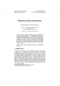
(a) von Neumann neighborhood

(b) Moore neighborhood

Figure 1: Two examples of a cell with a one-step update. The center cell examines its neighborhood and applies the update rule (in this case, it sets itself to the majority value of its neighbors). Dust (Warneke, Last, Liebowitz, & Pister, 2001). Each of these ideas proposes a network of very small, very numerous, interconnected units. These will likely have processing aspects similar to those of cellular automata. In order to understand how data mining might be performed by such “computational clouds”, it is useful to investigate how cellular automata might accomplish these same tasks. The purpose of this study is not to present a new, practical data mining algorithm, nor to propose an extension to an existing one; but to demonstrate that effective generalization can be achieved as an emergent property of cellular automata. We demonstrate that effective classification performance, similar to that produced by complex data mining models, can emerge from the collective behavior of very simple cells. These cells make purely local decisions, each operating only on information from its immediate neighbors. Experiments show that cellular automata perform well with relatively little data and that they are robust in the face of noise. The remainder of this paper is organized as follows. Section 1 provides basic background on cellular automata, sufficient for this paper. Section 2 describes an approach to using CA for data mining, and discusses some of the issues and complications that emerge. Section 3 presents some basic experiments on two-dimensional patterns, where results can be visualized easily, comparing CAs with some common data mining methods. It then describes the extension of CAs to more complex multi-dimensional data and presents experiments comparing CAs against other data mining methods. Section 4 discusses some related work, and Section 5 concludes.

1

Cellular Automata

Cellular automata are discrete, dynamical systems whose behavior is completely specified in terms of local rules (Toffoli & Margolus, 1987). Many variations on cellular automata have been explored; here will shall describe only the simplest and most common form, which is also the form used in this research. Sarkar (2000) provides a good historical survey. A cellular automaton (CA) consists of a grid of cells, usually in one or two dimensions. Each cell takes on one of a set of finite, discrete values. For concreteness, in this paper we shall refer to two-dimensional grids, although section 3.3 relaxes this assumption. Because we will deal with two-class problems, each cell will take on one of the values 0 (empty, or unassigned), 1 (class 1) or 2 (class 2). Each cell has a finite and fixed set of neighbors, called its neighborhood. Various neighborhood definitions have been used. Two common two-dimensional neighborhoods are the von Neumann neighborhood, in which each cell has neighbors to the north, south, east and west; and the Moore neighborhood, which adds the diagonal cells to the northeast, southeast, southwest and northwest2 . Figure 1 shows these two neighborhoods in two dimensions. In general, in a d-dimensional space, a cell’s von Neumann neighborhood will contain 2d cells and its Moore neighborhood will contain 3d − 1 cells. A grid is “seeded” with initial values, and then the CA progresses through a series of discrete timesteps. At each timestep, called a generation, each cell computes its new contents by examining the cells in its immediate neighborhood. To these values it then applies its update rule to compute its new state. Each cell follows the same update rule, and all cells’ contents are updated simultaneously and synchronously. A critical characteristic of CAs is that the update rule examines only its neighboring cells so its processing is entirely local; no global or macro grid characteristics are computed. These generations proceed in lock-step 2 In data mining terms, the von Neummann neighborhood allows each cell to be influenced only by immediately adjacent attribute values, whereas a Moore neighborhood allows adjacent pairwise interactions.

2

DRAFT -- DRAFT -- DRAFT -- DRAFT -- DRAFT --

Initial

Generation 2

Generation 3

Generation 4

Generation 20

Figure 2: Several generations of a cellular automaton (parabola target concept)

(a)

(b)

(c)

(d)

Figure 3: A 2D cellular automaton with the n4 V1 rule with all the cells updating at once. Figure 2 shows a CA grid seeded with initial values (far left) and several successive generations progressing to the right. At the far right is the CA after twenty generations and all cells are assigned a class. The global behavior of a CA is strongly influenced by its update rule. Although update rules are quite simple, the CA as a whole can generate interesting, complex and non-intuitive patterns, even in onedimensional space. In some cases a CA grid is considered to be circular or toroidal, so that, for example, the neighbors of cells on the far left of the grid are on the far right, etc. In this paper we assume a finite grid such that points off the grid constitute a “dead zone” whose cells are permanently empty.

2

Cellular Automata for Data Mining

We propose using cellular automata as a form of instance-based learning in which the cells are set up to represent portions of the instance space. The cells are organized and connected according to attribute value ranges. The instance space will form a (multi-dimensional) grid over which the CA operates. The grid will be seeded with training instances, and the CA run to convergence. The state of each cell of the CA will represent the class assignment of that point in the instance space. The intention is that cells will organize themselves into regions of similar class assignment. We use a simple voting rule that locally reduces entropy. A voting rule examines a cell’s neighbors and sets the cell according the number of neighbors that are set to a given class, but voting rules are insensitive to the location of these neighbors. In this work we use the von Neumann neighborhood because it is linear in the number of dimensions of the instance space, so it scales well. It is instructive to examine a simple example of a cellular automaton in action. Figure 3 shows the effect of a CA update rule called n4 V1. This rule examines each cell’s four neighbors and sets its class to the majority class. It is a stable rule in that once the cell’s class has been set it will not change. Figure 3a shows a grid with four cells initially set, two for each class. The remainder of the cells in the grid are blank, i.e., their class is unassigned. Informally, the effect of the rule is to spread the class activation outward in a diamond pattern from each set cell. Figures 3b and c show this progression after the first and second timesteps; Figure 3d shows the grid after it has been completely filled. The color of each cell indicates the

3


4

4

4

4

3.5

3.5

3.5

3.5

3

3

3

3

2.5

2.5

2.5

2.5

2

2

2

2

1.5

1.5

1.5

1.5

1

1

1

1

0.5

0.5

0.5

0.5

0

0 0

0.5

1

1.5

2

2.5

(a) Linear

3

3.5

4

0 0

0.5

1

1.5

2

2.5

3

3.5

4

0 0

(b) Parabolic

0.5

1

1.5

2

2.5

3

3.5

4

(c) Closed concave

0

0.5

1

1.5

2

2.5

3

3.5

4

(d) Disjunctive

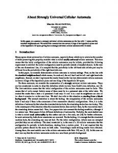
Figure 4: Four of the two-dimensional concept targets class that will be assigned to a point that falls into that grid position. The global effect of the nv V1 update rule is that each cell in the grid becomes assigned with the class of the nearest initial point as measured by Manhattan distance. The Manhattan distance aspect stems from the fact that the CA uses the von Neumann neighborhood, so each cell’s influence spreads outward along the two dimensions. The first neighbor of a cell that changes state, from empty to a class, will result in that cell changing state in the next timestep. Given the initial points in figure 3a, this results in the cell assignments shown in figure 3d. Note that in the experiments below, a different, more complex update rule is used. The rule, called n4 V1 nonstable, is a non-stable update rule in which a cell may change its class if the majority changes. Specifically, the rule is defined as:  0 : class 1 neighbors + class 2 neighbors = 0    1 : class 1 neighbors > class 2 neighbors n4 V1 nonstable = 2 : class 1 neighbors < class 2 neighbors    rand({1, 2}) : class 1 neighbors = class 2 neighbors where rand({1, 2}) selects randomly from the elements with equal probability.

3

Experiments in two dimensions

In the literature, CAs typically use only one or two-dimensions. They have been generalized to three and more dimensions, but complexity issues of space and time become problematic, and visualization is difficult. Because of this, the first experiments below were designed to illustrate and visualize the operation of cellular automata as a classification method and to compare them with well-known classifier induction algorithms.

3.1

Qualitative experiments in two dimensions

As a test, a set of two-dimensional geometric patterns of (approximately) increasing complexity were created: an axis-parallel line, a line of arbitrary slope, a parabola, a closed convex polygon, a closed concave polygon, and a disjunctive set of multiple closed concave polygons. Each target concept was generated in a square twodimensional plane x ∈ [0, 4], y ∈ [0, 4], sectioned into cells .05 on a side, producing a grid of 81 × 81 = 6561 cells. Figure 4 shows four of the target patterns. A two-class problem was created from each pattern by using the pattern as a boundary that divided the space. For example, for the parabolic pattern in 4b, points above the parabola were assigned class 1 and points below it are assigned class 2. For polygons, point interiors versus exteriors were used to determine classes. Examples were created from each problem by randomly sampling a cell and labeling each cell with the class of its region; in data mining terms, each example was a tuple hx, y, classi. A total of 6561 cells yielded 6561 total examples for each target concept. Varying numbers of training examples were sampled, as explained below. For comparison with cellular automata, several other common induction algorithms were chosen from the Weka package (Witten & Frank, 2000). J48, a decision tree induction algorithm, is a common and popular 4


4

4

4

3.5

3.5

3

3

3

2.5

2.5

2

2

2

1.5

1.5

1

1

1

0.5

0.5

0

0 0

0.5

1

1.5

2

2.5

3

3.5

4

0

0

1

(a) Parabolic target

2

3

0

4

4

4

3.5

3.5

3.5

3

3

3

2.5

2.5

2.5

2

2

2

1.5

1.5

1.5

1

1

1

0.5

0.5

0.5

0

0 0.5

1

1.5

2

2.5

3

(d) SMO hypothesis

3.5

4

1

1.5

2

2.5

3

3.5

4

3.5

4

(c) J48 hypothesis

4

0

0.5

(b) Training instances

0 0

0.5

1

1.5

2

2.5

3

(e) kNN hypothesis

3.5

4

0

0.5

1

1.5

2

2.5

3

(f) CA hypothesis

Figure 5: Two-dimensional parabolic target and the hypotheses generated by various learning methods. symbolic learning algorithm. kNN, an nearest-neighbor learning algorithm, was chosen to provide a “lazy” instance-based method to contrast with the CA. SMO, an implementation of support vector machines, was chosen because of their generally good performance.3 The CA used the n4 V1 nonstable rule discussed above. Space limitations prohibit showing all of these experiments, but figure 5 shows typical results with the parabolic pattern. Figure 5a shows the full target concept, and 5b shows a scatterplot of 200 data points randomly sampled from it, comprising a training set. Figures 5c-f shows the hypotheses generated by J48, SMO, kNN and CA, respectively. These diagrams were created by sampling 200 examples from the target concept then testing on the entire set4 Most of these results should be unsurprising. Because J48 is a decision tree learner which creates axisparallel splits in the instance space, its hypothesis region will always be composed of horizontal and vertical line segments. SMO was used with a kernel that could fit up to third degree polynomials, so it is able to model the target form, though its fit is not exact. Both kNN and CA are low-bias learners which have much greater latitude in approximating regions. Consequently their boundaries are usually more erratic and they risk over-fitting, but when irregular boundaries are required these methods can come closer to modeling the true boundary region. Note that although both are instance-space methods and their hypotheses look similar, the boundaries are not identical.

3.2

Quantitative results in two dimensions

The preceding diagrams are useful for visualization but they provide no estimates of modeling quality or variation due to sampling. For this we perform a standard data mining empirical validation: ten-fold cross3 Specifically, kNN was allowed to use up to five neighbors (-K 5), with cross-validation (-X) used to select k. SMO was used with a polynomial kernel with exponents up to 3 (-E 3). Otherwise, Weka’s default settings were used. 4 Strictly speaking, testing on an example set that includes the training examples is poor experimental methodlogy. This was only done for the visualization experiments so that the entire 2-D plane could be shown; the quantitative experiments used a stricter regimen.

5


100

90

90

80

80

80

70

70

70

60 50 40 30

50 40

50

100

200

150

250

300

350

400

450

0

500

0

50

100

90

90

80

80

70

70

60 50 40

0

300

350

400

450

500

0

0

50

100

150

200

250

300

350

400

450

500

Number of examples

Closed convex

50 40 CA kNN SVM J48

20

10

CA kNN SVM J48

60

30

CA kNN SVM J48

20

250

Closed concave

Accuracy

Accuracy

Linear

30

200

150

Number of examples 100

40

10

Number of examples 100

50

20

10 0

60

30

CA kNN SVM J48

20

10 0

60

30

CA kNN SVM J48

20

Accuracy

100

90

Accuracy

Accuracy

100

10 0

50

100

150

200

250

300

Number of examples

Parabolic

350

400

450

500

0

0

50

100

150

200

250

300

350

400

450

500

Number of examples

Disjunctive

Figure 6: Generalization performance on two-dimensional target concepts as a function of training set size validation of the example set using hold-one-out sampling. The first experiment was designed to test the sensitivity of CAs to the training set size. Because CAs are a non-parametric, low-bias method, we may expect them to be sensitive to the number of examples. In this experiment we performed ten-fold cross validation varying instance set sizes from 50 through 500 incrementing by 50. We measure the mean accuracy and standard deviation. The results are shown in figure 6. The error bars around each point mark the 95% confidence interval. Based on the accuracy figures, these patterns are approximately increasing in difficulty for all induction methods, with the disjunctive concept posing the greatest difficulty. All methods perform erratically if given only a few examples, with the confidence increasing steadily as more examples are provided. The CA method performs about as well as kNN, the other instance space method. SMO’s performance trails in many experiments, perhaps because its polynomial kernel cannot capture the irregular regions used here. The second experiment was designed to test the sensitivity to noise of cellular automata compared with the other modeling methods. Given the patterns above, the example set size was fixed at 100 points and class noise was injected randomly into the instance sets by inverting class labels. For example, with noise at 0.1, a randomly chosen 10% of the training instances would have their labels inverted. Using ten-fold cross-validation, the effect of this noise introduction was measured as the drop in accuracy. The results are shown in figure 7. All methods degrade with increasing amounts of noise, as should be expected. SMO, the support vector machine implementation, degrades most slowly. It is model based, so it has a higher bias than the other induction methods. The cellular automaton (CA) is more sensitive to noise and degrades similarly to the nearest neighbor (kNN) method; again, since they are low-bias methods they are more strongly influenced by individual noisy examples.

6


100

90

90

80

80

80

70

70

70

60 50 40 30

60 50 40 30

CA kNN SVM J48

20

10

0

0

0.05

0.1

0.15

0.2

0.25

0.3

0.35

0.4

0

0.05

0.1

90

80

80

70

70

60 50 40 30

0

0.25

0.3

0.35

0.4

0

0

0.05

0.1

0.15

0.2

0.25

0.3

0.35

0.4

Noise

Closed convex

50 40 CA kNN SVM J48

20

10

CA kNN SVM J48

60

30

CA kNN SVM J48

20

0.2

0.15

Closed concave

Accuracy

Accuracy

Linear 90

40

10

Noise 100

50

20

Noise 100

60

30

CA kNN SVM J48

20

10 0

Accuracy

100

90

Accuracy

Accuracy

100

10 0

0.05

0.1

0.15

0.2

0.25

0.3

0.35

0.4

0

0

0.05

0.1

Noise

Disjunctive

0.2

0.15

0.25

0.3

0.35

0.4

Noise

Parabolic

Figure 7: Generalization performance on two-dimensional target concepts as a function of class noise

3.3

Multi-dimensional data mining

Cellular automata are a natural fit to two dimensional problems. Up to this point we have dealt with CAs in two dimensions. To be a general data mining method, they must be extended to multiple dimensions. Several issues arise when doing so. Grid definition. One issue is how to map the instance space onto a grid so as to define cell neighborhoods for the CA. A solution is to assign one grid dimension to each attribute. For d attributes, we create a d-dimensional grid for the CA and partition each grid dimension by the attribute’s values. Each grid point (cell) then corresponds to a specific value or range of values in instance space. Each cell is connected to 2d neighbors. For ordinal attributes, the values naturally form a gradient which can constitute a neighborhood. Continuous attributes can be discretized so that each cell is responsible for a particular range of values. Thus, for example, a problem with six independent variables would give rise to a six-dimensional grid. Grid size. Another issue is how large the grid should be, i.e., how may cells each attribute should occupy. One solution is to assume that adjacent cells should be able to distinguish the minimum non-zero difference between data items. To do this we can simply measure the range of an attribute’s values in the data, find the minimum distance between any two adjacent values, then use this value to determine the size of the grid along that dimension: max(A) − min(A) Number of cells for attributeA = minimum distance This assures a minimal separation among attribute values.

7


Domain abalone breast-wisc iris new-thyroid pima

Classes 2 (34/66) 2 (35/65) 2 (50/50) 2 (86/14) 2 (35/65)

Attributes 3 9 4 5 8

Instances 4177 683 100 215 768

kNN 78.9 ± 2.4 96.8 ± 2.5 100 ± 0 97.5 ± 3.5 74.1 ± 3.8

Dtree 81.7 ± 2.0 95.7 ± 1.8 99 ± 6.3 95 ± 6.2 72.9 ± 4.3

SVM 80.2 ± 1.9 96.2 ± 2.1 100 ± 0 96 ± 4.6 76.4 ± 3.1

CA 79.1 ± 2.5 96.4 ± 3.0 99 ± 3.2 95 ± 3.3 73.1 ± 3.4

Table 1: Domains Convergence. Another issue is how many generations to let the CA run. When using a stable (i.e., monotonic) update rule, in which cells do not change state once they are set, the CA may simply be run until no new cells change state. With a non-stable update rule, oscillation may occur at boundary cells, so the CA as a whole may never stabilize. This is addressed by running the CA until no cells are left empty (unassigned), and then continuing until either no changes are made or a fixed threshold is exceeded. In the experiments below, the CA was run for a maximum of ten generations once all cells were assigned. Table 1 describes the domains used in experiments and the accuracy scores achieved by each technique. Each of the domains was taken from the UCI data repository (Hettich, Blake, & Merz, 1998), though some were modified as described below. 1. Abalone is a version of the Abalone domain in which abalone are described by the length, diameter and height of the abalone shell. The dependent variable is the number of rings, discretized into < 9 rings (class 1) and ≥ 9 rings (class 2). 2. Breast-wisc is a two-class problem in which the task is to classify breast tumor instances into benign (class 2) and malignant (class 4). 3. Iris is a two-class problem using only instances of class 1 (Iris Setosa) and 2 (Iris Versicolour). 4. New-thyroid is a variant of the Thyroid domain using only classes 1 (Normal) and 3 (Hypo). 5. Pima is a database for diagnosing diabetes mellitus from a population of Pima Indians. It is unaltered from the UCI version. The size of the domains was constrained by practical time and space considerations. Simulating CAs with hundreds of thousands of cells is time consuming on a serial computer. Since the number of cells is proportional to the number of dimensions, problems were chosen with relatively few (less than ten) attributes. The CA was given a total of 300,000 cells, which were allocated to each attribute on the basis of their value separations, as described in the discussion of “grid size,” above. The CA was then seeded with examples from the training set, and the CA run to convergence. The test set examples were then evaluated by mapping them to cells in the resulting CA and checking the true class against the cell’s class. Strict statistical testing (e.g., T-tests) was not performed with these results. The intention was not to show that CAs are superior to other methods, but to demonstrate that they can achieve similar generalization performance. Indeed, all methods tested here achieved fairly close levels of accuracy on these domains. The mean accuracies of the CA trail slightly on new-thyroid and pima, but the standard deviations on all methods are high enough that the differences are likely insignificant. These basic experiments show that a cellular automaton is able to demonstrate performance approximately equal to that of other data mining techniques on these domains.

4

Related Work

The use of CAs presented here is a form of instance-space classification, whereby the classifier operates directly in the instance space of the data rather than creating a model of the data. Instance-space classifiers are not new in data mining. Such classifiers have long been prevalent in machine learning, pattern recognition and statistics in the form of instance-based learning and nearest neighbor classifiers (Aha, Kibler, & Albert, 1991; Duda, Hart, & Stork, 2000). These classifiers store some portion of the labeled instances presented to 8


them. Given a new instance to be classified, they retrieve one or more close neighbors in the instance space and form a class hypothesis from the labels of these neighbors. However, these methods are distinguished from CAs in that they are not strictly local : there is no notion of a bounded and fixed neighborhood, and an instance’s nearest neighbor may be arbitrarily far away. As such, they are not bounded in their connectivity or in the information they use. Cellular automata have been employed in data mining and pattern recognition in various ways. In reviewing prior work, it is important to distinguish between work that uses a CA as a performance engine versus work that uses a CA as an induction technique. Much work is of the first type, in which a CA is developed or evolved, usually by a genetic algorithm or a genetic programming technique, to solve a particular task (Ganguly, 2004; Maji, Sikdar, & Chaudhuri, 2004). In such work, the induction is performed by a separate process, which searches a space of possible cellular automata. The output of the induction process is a specific cellular automaton adapted to perform the task characterized by the set of examples. The second approach uses CAs as an induction technique. Ultsch’s work (2000, 2002) is the closest in spirit to the work described in this paper. He described “Databots” as a kind of autonomous minirobot that can roam across a two-dimensional grid called a UD-Matrix. Their actions are influenced by their neighbor’s grid contents. One significant difference with the work described here is that the grid was simple but the messages passed between nodes—n-dimensional input vectors—were complex. Ultsch applied his technique to a dataset describing Italian olive oils and showed that it was able to cluster the oils geographically by their point of origin. However, Ultsch did not compare his method to other techniques, and did not address questions of how the method would scale to more than two dimensions and how those dimensions should be defined for problems that are not inherently spatial or geographical.

5

Discussion

As stated earlier, the purpose of this study is to demonstrate that effective classification performance can be achieved by very simple (cellular) automata that make purely local decisions. To the best of our knowledge, this has not been demonstrated in prior work. We show that effective classification performance, similar to that produced by complex data mining models, can emerge from the collective behavior of very simple cells. These cells make local decisions, each operating only on information from its immediate neighbors, and each performs a simple, uniform calculation. Many of the choices made in this initial work were intentionally simple and straightforward. Open issues remain concerning alternative choices. We have defined grid neighborhoods such that every attribute is a separate dimension. This makes mapping instances onto cells very convenient, but the grid size is exponential in the number of attributes. There are other ways to accomplish this mapping, and future work should experiment with this. Similarly, the domains chosen used only continuous attributes because they could be discretized into ranges so that a grid could be constructed easily. Other data mining methods (e.g., logistic regression) make similar requirements of attributes. However, a general data mining method should ideally handle discrete and ordinal attributes as well, and future work should address this. It is likely that techniques from nearest neighbor methods could be used, since they must address similar representation problems. For simplicity and efficiency we have chosen the von Neumann neighborhood with a simple (but nonstable) majority-vote update rule. This seems to perform reasonably well in practice, but future work could experiment with other update rules to determine their effects. This study is not intended to promote an immediately applicable data mining technique. Although CA hardware is available now, it is still not commonplace, and simulating networks of cells on a serial computer is not a good use of such processing power. However, nanotechnology is becoming increasingly important, with researchers exploring ideas such as motes, Smart Dust and Utility Fog (Warneke et al., 2001; Hall, 2001). These concepts involve very large collections of tiny interconnected processing units. It is likely that units will collectively perform some form of data mining and self-organization, either as their sole purpose or as an instrumental part of it. We hope that the ideas in this paper can serve as a foundation for such work.

9


References Aha, D. W., Kibler, D., & Albert, M. K. (1991). Instance-based learning algorithms. Machine Learning, 6, 37–66. Bandini, S., & Mauri, G. (Eds.). (1996). Proceedings of the Second Conference on Cellular Automata for Research and Industry. Springer-Verlag. Benyoussef, A., HafidAllah, N. E., ElKenz, A., Ez-Zahraouy, H., & Loulidi, M. (2003). Dynamics of HIV infection on 2d cellular automata. Physica A: Statistical Mechanics and its Applications, 322, 506–520. Brady, M., Raghavan, R., & Slawny, J. (1989). Probabilistic cellular automata in pattern recognition. In International Joint Conference on Neural Networks, pp. 177–182. Duda, R. O., Hart, P. E., & Stork, D. G. (2000). Pattern Classification (Second edition). Wiley Interscience. Ganguly, N. (2004). Cellular Automata Evolution: Theory and Applications in Pattern Classification and Recognition. Ph.D. thesis, Bengal Engineering College. Gardner, M. (1970). Mathematical games: The fantastic combinations of John Conway’s new solitaire game ”life”. Scientific American, 223, 120–123. Available: http://hensel.lifepatterns.net/ october1970.html. Hall, J. S. (2001). Utility fog: The stuff that dreams are made of. Available: http://www.kurzweilai. net/articles/art0220.html?m=18. Hettich, S., Blake, C., & Merz, C. (1998). UCI repository of machine learning databases.. http://www.ics. uci.edu/∼mlearn/MLRepository.html. Maji, P., Sikdar, B. K., & Chaudhuri, P. P. (2004). Cellular automata evolution for distributed data mining. Lecture Notes in Computer Science, 3305, 40–49. Ramos, V., & Abraham, A. (2003). Swarms on continuous data. In Proceedings of CEC-03 - Congress on Evolutionary Computation, pp. 1370–1375. IEEE Press. Sarkar, P. (2000). A brief history of cellular automata. ACM Computing Surveys, 32 (1). Sipper, M., Capcarrere, M. S., & Ronald, E. (1998). A simple cellular automaton that solves the density and ordering problems. International Journal of Modern Physics, 9 (7). Sullivan, A. L., & Knight, A. K. (2004). A hybrid cellular automata/semi-physical model of fire growth. In The 7th Asia-Pacific Conference on Complex Systems. Syphard, A. D., Clark, K. C., & Franklin, J. (2005). Using a cellular automaton model to forecast the effects of urban growth on habitat pattern in southern California. Ecological Complexity, 2, 185–203. Toffoli, T., & Margolus, N. (1987). Cellular Automata Machines. MIT Press. Ultsch, A. (2000). An artificial life approach to data mining. In Proc. European Meeting of Cybernetics and Systems Research (EMCSR). Ultsch, A. (2002). Data mining as an application for artificial life. In Proc. Fifth German Workshop on Artificial Life, pp. 191–197. Warneke, B., Last, M., Liebowitz, B., & Pister, K. S. J. (2001). Smart dust: Communicating with a cubic-millimeter computer. Computer, 34 (1), 44–51. Witten, I., & Frank, E. (2000). Data mining: Practical machine learning tools and techniques with Java implementations. Morgan Kaufmann, San Francisco. Software available from http://www.cs.waikato. ac.nz/∼ml/weka/. Wolfram, S. (1994). Cellular Automata and Complexity: Collected Papers. Westview Press. Wolfram, S. (2002). A New Kind of Science. Wolfram Media, Inc., Champaign, IL.

10
