Modeling of asynchronous cellular automata with fixed-point attractors for pattern classification Biswanath Sethi∗
Sukanta Das
Department of Information Technology Bengal Engineering and Science University, Shibpur, Howrah, West Bengal, India-711103. Email:
[email protected],
[email protected] * Corresponding author Abstract—This paper addresses a detail characterization of the one-dimensional two-state 3-neighborhood asynchronous cellular automata (ACA) having multiple fixed-point attractors with the target to model this class of CA for designing efficient pattern classifier. The cells of ACA are independent, and they are updated independently. When an ACA cell is updated, it reads the states of its neighbors and then updates its state following the state transition function. The ACA rules are characterized considering an arbitrary cell is updated in each time step. A theorem is designed for the identification of ACA with only fixed-point attractors. From this theorem we get 146 out of 256 ACA in two-state 3-neighborhood interconnection which always approach towards fixed-Point attractors. To identify individual fixed-point attractors, a directed graph, namely Fixed-point graph (FPG) is proposed. The FPG guides us to point out the ACA having multiple fixed-points attractors. There are 83 such ACA (out of 146 ACA with only fixed-point attractors) that are utilized to design efficient pattern classifier. Finally, the proposed classifier is tested with real-life data sets, and it is observed that the performance of the proposed ACA based classifier is always better than that of traditional CA based classifier and is also better than many other well-known pattern classifiers. Index Terms—Cellular automata model, asynchronous cellular automata (ACA), fixed-point attractor, Fixed-point graph (FPG), pattern classifier.
I. I NTRODUCTION With the increase of computing power, the researchers have been showing their interest on the study of global behavior of cellular automata (CA). The CA have become popular tool to simulate various real-world systems. CA were originally introduced as an abstract mathematical model capable of selfreproduction [12]. They are defined by a lattice of cells and a local rule by which state of a cell is determined as a function of the state of its neighbors. In early 1980, the CA structure was simplified, and a two-state, 3-neighborhood CA structure was proposed on an one-dimensional lattice [13]. The researchers working with VLSI design and test have got attracted to this type of CA due to their simplicity and ease of hardware implementations [1]. This contribution also concentrates on such one-dimensional two-state 3-neighborhood CA. While characterizing the CA, a set of CA states have been identified, toward which neighboring states asymptotically approach in the course of dynamic evolution, called attractors [1], This work is supported by DST Fast Track Project Fund (No.SR/FTP/ETA0071/2011)
978-1-4799-0838-7/13/$31.00 ©2013 IEEE
[14]. The attractors can be of length 1 (fixed-point attractor) or of length greater than 1 (multi-state attractor). The CA with multiple fixed-point attractors have been targeted to design effective solutions for patten classification [1]. The characterization of CA for pattern classification has received special attention for cost effective solutions of real life applications. The CA, contributing with this context, are addressed in [2], [3], [5]–[8]. However, all such contributions have dealt with synchronous CA, where all the CA cells are forced to be updated simultaneously. On the other hand, in asynchronous CA (ACA) the cells are independent, and as a result, the cells are free to get updated independently [4], [9]. This independence property of ACA cells may affect the performance of ACA while they are utilized to address some real life problems. The ACA, however, have rarely been considered to solve pattern classification problem. Two dimensional ACA are studied in [10], [11] to utilize them for pattern classification. To our knowledge, no target has been taken to study one-dimensional ACA as pattern classifier. In this scenario, we concentrate on characterization of ACA in one-dimensional two-state 3-neighborhood interconnection, with the target to design an efficient model for pattern classification. The ACA with multiple fixed-point attractors are utilized for pattern classification. We refer such ACA as multiple attractor ACA (MAACA). Here, we design 2-class classifier. We explore the essential properties of attractors that enable us for such characterization. A theorem has been reported for the identification of ACA with fixed-point attractors. One of the major contributions of this work is, it introduces the idea of Fixed-point graph to identify the fixed-point attractors of ACA. An algorithm is also developed to find the fixedpoint attractors from the graph. Finally, the pattern classifier is designed and tested with real-life data sets. It is shown that performance of ACA based classifier is much better than that of traditional (that is, synchronous) CA based classifier. Moreover, the proposed classifier is very much competitive with other well-known classifier, even better than them in many cases. The next section introduces the preliminaries of ACA and some definitions which are relevant for the current work. Section III reports the characterization of ACA. A theorem and algorithms for characterization are addressed in this section.
311
TABLE II R ELATIONSHIP BETWEEN ith AND (i + 1)th RMT S
TABLE I L OOK - UP TABLE FOR RULE 36, 77 AND 219 PS : (RMT ) (i)NS : (ii)NS : (iii)NS :
111 (7) 0 0 1
110 (6) 0 1 1
101 (5) 1 0 0
100 (4) 0 0 1
011 (3) 0 1 1
010 (2) 1 1 0
001 (1) 0 0 1
000 (0) 0 1 1
Rule
ith RMT 0, 4 1, 5 2, 6 3, 7
36 77 219
The design of pattern classifier are devised in section IV. The algorithm for the design of pattern classifier is also reported. The performance of the proposed scheme with other are also reported in this section. II. P RELIMINARIES
OF
ACA
Cellular automaton (CA) is a discrete dynamical system which evolves in discrete time and space. A CA consists of a lattice of cells, each of which stores a boolean variable at time t, that refers to the present state of the CA cell [13]. The next state of a cell of one-dimensional two-state 3-neighborhood CA is determined by the present states of left, self and right neighbors. Hence, t t Sit+1 = f (Si−1 , Sit , Si+1 ) t Si−1 ,
(1)
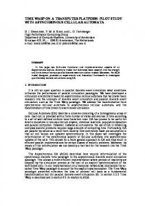
where f is the next state function; and are the present states of the left neighbor, self and right neighbor of the ith CA cell at time t respectively. A collection of (local) states S t (S1t , S2t , · · · , Snt ) of cells at time t is referred as a configuration or a (global) state of the CA at t. The function f : {0, 1}3 7→ {0, 1} can be expressed as a look-up table (see TABLE I). The decimal equivalent of the 8 outputs is called ‘rule’ [13]. There are 28 = 256 CA rules in two-state 3-neighborhood dependency. Three such rules (36, 77 and 219) are shown in TABLE I. From the view point of Switching Theory, a combination of the present states can be considered t t as the Min Term of a 3-variable (Si−1 , Sit , Si+1 ) switching function. So, each column of the first row of TABLE I is referred to as Rule Min Term (RMT). The column (011) is the RMT 3. The next states corresponding to this RMT are 0 for rule 36 and, 1 for rule 77, and 1 for rule 219 (TABLE I). When the left most and right most cells of an n-cell CA are t the neighbors of each other (that is, S0t = Snt and Sn+1 = S1t ), the CA is called periodic boundary CA. Traditionally, the cells of a CA are updated simultaneously. In asynchronous update, on the other hand, the cells are considered as independent and so, updated independently. We have considered here that a single arbitrary cell is updated in each time step. Such CA are referred as asynchronous cellular automata (ACA). This work deals with one-dimensional twostate 3-neighborhood ACA under periodic boundary condition. The next state of a synchronous CA is determined by the rule only. However, in ACA, the next state does not only depend on the rule, but also on the cell which is being updated randomly. Fig. 1 shows state transition diagram of 4-cell rule 219 ACA in periodic boundary condition. The cells, updated randomly during state transition, are noted over arrows. An ACA state can be viewed as a sequence of RMTs. For example, the state 1110 in periodic boundary condition can Sit
t Si+1
(i + 1)th RMT 0, 1 2, 3 4, 5 6, 7
be viewed as h3765i, where 3, 7, 6 and 5 are corresponding RMTs on which the transitions of first, second, third and fourth cell can be made. To get a sequence of RMTs for a state, we consider an imaginary 3-bit window that slides over the state. The window contains a 3-bit binary value which is equivalent to RMT. To get the ith RMT, the window is loaded with (i − 1)th , ith and (i + 1)th bits of the state. The window slides one bit right to report the (i + 1)th RMT. Now the current content of the window is ith , (i + 1)th and (i + 2)th bit of the state. In the sequence of RMTs, however, two consecutive RMTs are related. If 5 (101) is the ith RMT in some sequence, then (i + 1)th RMT is either 2 (010) or 3 (011). Similarly, if 0 (000) or 4 (100) is the ith RMT, then 0 (000) or 1 (001) is the (i + 1)th RMT. The relations of two consecutive RMTs in a sequence of RMTs are noted in TABLE II. These relations play an important role in the design of pattern classifier, reported in this paper. Definition 1: An RMT r of a rule is active if an ACA cell flips its state (1 to 0 or 0 to 1) on r. Otherwise, the RMT r is passive. For example, RMT 1 (001) of rule 219 (see TABLE I) is active. Because, while a cell is acting on that particular RMT, then the cell’s present state is 0 and next state for the rule is 1. Hence, transition occurs. So, it can be said that if the middle bit of an RMT is unequal with the RMT value, the RMT is active. RMT 7 (111) of rule 219, on the other hand, is passive. Definition 2: A fixed-point attractor is an ACA state, next state of which is the state itself for any style of update of cells. That is, if an ACA reaches to a fixed-point attractor, the ACA remains in that particular state forever. In Fig. 1, the states 1101, 0111, 1111, 1011 and 1110 are fixed-point attractors for rule 219 ACA. The RMT sequence for the state 1111 is h7777i. The next state of 1111 is always 1111 for the update of any cell in any sequence. The RMT 7 is passive for rule 219. It can be observed that the RMTs in the RMT sequence of a fixed-point attractor are to be passive. Hence, we get the following lemma. Lemma 1: Rule R ACA forms a fixed-point attractor with state S if the RMTs of the RMT sequence of S are passive. Since there are five, attractors in 4-cell rule 219 ACA, we can find five basins of attraction (Fig. 1). An attractor is the representative of the corresponding basin. If not specified otherwise, we shall refer fixed-point attractor as just attractor in our further discussion. III. C HARACTERIZATION
OF
ACA
This section reports the properties of ACA to explore the fixed-point attractors. The proposed characterization is based
312
0000 1
0001
0100
0001
0101
1
1
1000
1001
3 0011
1101
1111
2 0001 3 0011 2 0111
(a)
1/2/3/4 (c)
1/23/4 (b)
2
0001 1 1001 3
4
0000 1 1000 4
1000 1 0000 1
1001
1000 4 1001
3 1011 1/2/3/4 (d)
Fig. 1.
2
2
4
1100
1100
3
0010
1000
2
2
0110
1100 3
1
1110
1010 1 0010 3 0110 4
1001 1 1001 4 1000 2 1100 3
1/2/3/4 (e)
A state transition diagram of 4-cell rule 219 ACA.
on a theorem and algorithms. The theoretical foundation is thus evolved and then employed to identify fixed-point attractors. A. ACA with only fixed-point attractors The following theorem states the necessary conditions of ACA, having only fixed-point attractors. Theorem 1: Rule R ACA converges to fixed-point attractor if (i) RMT 0 (RMT 7) of R is passive and RMT 2 (RMT 5) is active, or (ii) RMTs 0 and 7 are passive and RMT 2 or 5 is active, or (iii) RMTs 0, 1, 2, and 4 (RMTs 3, 5, 6, and 7) are passive and RMT 3 or 6 (RMT 1 or 4 ) is active, or (iv) RMTs 1, 2, 4, and 5 (RMTs 2, 3, 5 and 6) are passive. Proof: Proof of case (i): Let us consider RMT 0 of R is passive and RMT 2 is active. We shall show that the rule R ACA can reach to a fixed-point attractor from any initial state. Since RMT 0 is passive, the all-0 state (RMT sequence h00 · · · 0i) is a fixed-point attractor. In any other state (except all-1), a sequence of consecutive 1s guided by 0s can always be found. Consider, RMT 7 of R is active. Now in such a state (like · · · 0111110 · · ·), we can find RMT 7 in its corresponding RMT sequence. If a cell with RMT 7 is selected to update, in that case, the sequence of consecutive 1s is divided into two sub-sequences of consecutive 1s guided by 0s. The new sequences have less number of 1s (like · · · 0111110 · · · → · · · 0101110 · · ·). After a number of similar updates, we can get a state with a number of single 1 and two consecutive 1s guided by 0s. A cell has state 1 with left and right neighbor’s states as 0s (010) implies that the cell can act on RMT 2. Since RMT 2 is active, all such cells can reach to state 0. So, finally, we get either the all-0 state (that is, the ACA is converged to all-0), or a state with two consecutive 1s guided by 0s (· · · 001100 · · ·). In second case, the RMT sequence contains RMT 0 and RMTs 1, 3, 6 and 4. If RMTs 1, 3, 4 and 6 are passive, the state · · · 0110 · · · itself is a fixed-point attractor. Otherwise, the ACA can reach to all-0 (fixed-point) attractor after some update of cells. Hence, from an arbitrary
state with sequences of consecutive 1s guided by 0s, the ACA can reach to a fixed-point attractor. The all-1 state is a special state which contains no 0. However, if an arbitrary cell is updated, then we can get a 0, and then the new state can reach to fixed-point attractor with the above logic. Now consider, RMT 7 is passive. Then, the all-1 state (RMT sequence h77 · · · 7i) is another fixed-point attractor. A state with a sequence of consecutive 1s guided by 0s contains RMTs 3 and 6. If any one of them is active, the ACA with that state can reach to all-0 fixed-point. If both (RMT 3 and 6) are passive but RMT 1, 4 or 5 is active, the ACA can reach to all-1 fixed-points. If all RMTs except 2 are passive, then the state itself is a fixed-point attractor. Hence, the rule R ACA that can reach to fixed-point attractors from any initial state if RMT 0 of R is passive and RMT 2 is active. While RMT 7 is passive and RMT 5 is active (and the rest RMTs are active or passive) it can be shown by similar logic that the rule R ACA converge to fixed-point attractors Proof of case (ii): While RMTs 0 and 7 of R are passive and RMT 2 or RMT 5 is active, the ACA converges to fixed-point attractor. This proof can obviously followed from the proof of case (i). Proof of case (iii): Consider RMTs 0, 1, 2 and 4 of R are passive. Then, the states where two 1s are separated by at least two consecutive 0s (like · · · 001000100 · · ·) are fixedpoint attractors, because the corresponding RMT sequences of these states contain only RMTs 0, 1, 2 and 4 (Lemma 1). Now consider a state which contains two or more consecutive 1s. Therefore, the corresponding RMT sequence of the state contains RMTs 3, 7 and 6 (along with others). If RMTs 3 or 6 is active, the number of 1s can be reduced to a single 1 separated by 0s during evolution of the ACA. The resultant state is a fixed-point attractor if corresponding RMT sequence contains RMTs 0, 1, 2 and 4 only. If the resultant state (like · · · 001010 · · ·) contains any other RMT which is active (except 3 or 6) then updating the cells properly, we can reach to a state which is a fixed-point attractor. While RMTs 3, 5, 6, and 7 are passive, the states where two 0s are separated by at least two consecutive 1s (like · · · 11011011 · · ·) are fixed-point attractors because the corresponding RMT sequences of these states contain RMTs 3, 5, 6 and 7 only (Lemma 1). Now consider a state which contains two or more consecutive 0s. Therefore, the corresponding RMT sequence of state contains RMTs 4, 0 and 1 (along with other). If RMT 1 or 4 is active, the number of 0s can be reduced to single 0 separated by 1s during the evolution of the ACA. The resultant state is a fixed-point attractor if corresponding RMT sequence contains RMT 3, 5, 6, 7 only. If the resultant state contains any other RMT which is active (except RMT 1 or 4) then we can reach to a fixed-point attractor. Proof of case (iv): Consider RMTs 1, 2, 4 and 5 of R are passive. We shall next show that from any state, the ACA can reach to a fixed-point attractor while RMT 0, 3, 6, or 7 or none is active. Let us consider RMTs 0 and 7 are active. Now, from all-0 state, updating cell with RMT 0
313
we can reach to 0101 · · · after a number of time steps. The state 0101 · · · is a fixed-point attractor. The transitions are : 0000 · · · → 0100 · · · → · · · → 0101 · · ·. Similarly, from all-1 state, the ACA can reach to 0101 · · · 01 or 0101 · · · 011 (depending on the number of cells). The state 0101 · · · 01 is itself a fixed-point attractor and 0101 · · · 011 can be a fixed-point attractor if RMTs 3 and 6 are passive. If RMT 3 or 6 is active, the ACA can obviously reach to a fixed-point attractors. Now it can easily be shown that the ACA can reach to a fixed-point attractor from any state. Lastly, it can also be shown that rule R ACA can reach to a fixed-point attractor, if RMTs 2, 3, 5 and 6 are passive. We omit the detail steps of this proof because the rationale is similar with other cases. There are 64 rules where the RMT 0 is passive and RMT 2 is active (Theorem 1(i)). Similarly, identifying this way theorem 1 dictates that there are 146 ACA out of 256, which always approach to some fixed-point attractors. Such ACA rules are listed in TABLE III. Example 1: Let us consider the rule 36 ACA, in which RMTs 0, 1, 2 and 4 are passive. Therefore, the rule satisfies the condition for convergence to fixed-point attractor (Theorem 1 (iii)). Here, we assume number of cells are 4 and the initial state is 1111. The ACA can reach to a fixed-point attractor after some random update of cells from the initial state. One possible transition is: 1111(1) → 0111(4) → 0110(4) → 0110(2) → 0010 (the cell updated in a step is noted in bracket). TABLE III T HE RULES OF ACA WHICH ALWAYS APPROACH TOWARDS FIXED - POINT ATTRACTORS
0 16 42 68 80 96 122 141 163 171 179 187 197 208 222 230 238 246 254
2 18 44 69 82 98 128 144 164 172 180 188 200 210 223 231 239 247 255
4 24 48 72 88 100 130 146 165 173 181 189 202 216 224 232 240 248
5 26 50 74 90 104 132 152 166 174 182 190 203 217 225 233 241 249
8 32 56 76 92 106 133 154 167 175 183 191 204 218 226 234 242 250
10 34 58 77 93 112 136 160 168 176 184 192 205 219 227 235 243 251
12 36 64 78 94 114 138 161 169 177 185 194 206 220 228 236 244 252
13 40 66 79 95 120 140 162 170 178 186 196 207 221 229 237 245 253
B. Identification of fixed-point attractors Following Theorem 1, we can get the list of ACA which always converge to fixed-point attractors (TABLE III). However, the individual attractors of ACA are not identified. To utilize ACA as pattern classifier, one has to identify the attractors. This subsection reports the concept of Fixed-point graph (FPG) to identify the attractors. The FPG is a directed graph, where the nodes represent the passive RMTs. To get
1 2
3 6
4 Fig. 2.
5 Fixed-point graph (FPG) of rule 77 ACA
FPG for some ACA, we first identify the passive RMTs of the corresponding rule. As a next step, a forest considering the passive RMTs as individual nodes is formed. Now, we draw an edge from node u to node v, if u and v are related following TABLE II. For example, if RMTs 1, 2 and 5 are passive, then we can draw directed edges from node 1 to node 2, node 2 to node 5 and node 5 to node 2. But we can not draw the directed edge from node 1 to node 5, as RMT 1 and RMT 5 are not related (see TABLE II). We next propose an algorithm that constructs FPG of a given ACA rule. Algorithm 1: Construction of FPG Input: Rule R, TABLE II. Output: Fixed-point graph (G) with all passive RMTs are its vertices. Step 1. Point out the passive RMTs of R Step 2. Make forest with passive RMTs of R Step 3. For each vertex u repeat step 4 and step 5. Step 4. Find the next possible RMTs from TABLE II. Step 5. If the next possible RMT is a vertex v, then draw a directed edge from u to v Step 6. Report the graph as FPG Example 2: This Example illustrates the steps of Algorithm 1. Let us consider rule 77 ACA. Here, the passive RMTs are 1, 2, 3, 4, 5 and 6 (see TABLE I). As per step 2 of Algorithm 1, the vertices of the graph are 1, 2, 3, 4, 5 and 6 (see Fig. 2). Now considering the first vertex as vertex 1, we find the next RMTs of vertex 1 are RMT 2 and 3 (from TABLE II). As these two RMTs are also vertices, we draw directed edges from vertex 1 to both vertices 2 and 3 (see Fig. 2). Similarly, for vertex 3 the next possible RMTs are 6 and 7. But only one directed edge is possible from vertex 3 to vertex 6, since vertex 7 is absent (Fig. 2). After the construction of directed edges for all the vertices, the graph is the desired FPG. Fig. 2 is the FPG, resulted from the Algorithm 1 of rule 77 ACA. Following Algorithm 1, we can get the FPGs for the rules of ACA, which always approach to some fixed-point attractors. Algorithm 2, reported next, provides the procedure for counting the number of attractors from a FPG of a particular ACA. For each vertex in the FPG, we count number of cycles of length equal to the ACA size. The sum of all cycles for each vertex is the total number of fixed-point attractors for that particular ACA.
314
Algorithm 2: Counting Attractors Input : FPG (G) from Algorithm 1, n (CA size) Output: Number of fixed-point attractors Step 1. For each vertex v of (G), repeat steps 2 and 3. Step 2. Find whether v can be reached after exploring (n-1) vertices of (G) Step 3. If there are m ways to return back to v, add this m with the total no. of fixed-point attractors to be reported. Step 4. If no such path is found, a fixed-point attractor can not be formed with vertex v. Step 5. Report the total no. of fixed-point attractors. Example 3: This Example illustrates the execution steps of Algorithm 2. Let us consider, for the graph G (Fig. 2), we count the number of fixed-point attractors for 4 cell ACA. Starting from vertex 1, the vertex 1 can be reached after exploring vertices 3, 6 and 4 (step 2 of Algorithm 2). The path is 1 → 3 → 6 → 4 → 1 (Fig. 2). Similarly, other cycles of length 4 (as 4 cell ACA) in G can be found, and the total cycles of length 4 are the total number of fixed-point attractors in G. The cycles of length 4 in G (Fig. 2) are: 1) 1 → 3 → 6 → 4 → 1 2) 3 → 6 → 4 → 1 → 3 3) 6 → 4 → 1 → 3 → 6 4) 4 → 1 → 3 → 6 → 4 5) 2 → 5 → 2 → 5 → 2 6) 5 → 2 → 5 → 2 → 5 Hence, the total number of attractors in G is 6 (see Fig. 2). TABLE IV T HE RULES OF ACA WITH MULTIPLE FIXED - POINT ATTRACTORS (MAACA) 4 72 95 138 162 178 194 206 220 236 250
5 76 100 140 164 180 196 207 221 237 252
12 77 104 141 166 182 197 208 222 238 254
13 78 128 144 168 184 200 210 223 240
36 79 130 146 170 186 202 216 224 242
44 92 132 152 172 188 203 217 228 244
68 93 133 154 174 190 204 218 232 246
69 94 136 160 176 192 205 219 234 248
P
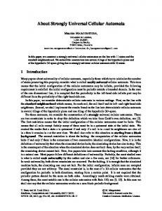
II I Memory
Fig. 3.
OF CLASSIFIER
An n-cell ACA with multiple fixed-point attractors (MAACA) can be viewed as a natural classifier. It classifies a set of patterns into different distinct classes, each class contains set of states of the attractor basin. For the identification
MAACA based classification strategy
Example 4: Let the MAACA of Fig. 1 be employed to classify patterns into two classes (say 1 and 2), where class 1 is represented by the states of three attractor basins and class 2 is represented by the states in the rest of basins. Let the attractors 1111, 0111 and 1110 be for class 1 and the rest attractors 1101 and 1011 be for class 2. Hence, the MAACA of Fig. 1 can act as 2-class pattern classifier. The design of MAACA based 2-class classifier for pattern classification demands the proper distribution of the patterns among the CA attractor basins. The design of classifier for two pattern sets P1 and P2 should ensure that elements of one class (say P1 ) are covered by a set of attractor basins that do not include any member from the class P2 . However, for real-life data sets, the attractor basins may mix up the patterns of two classes. Therefore, the primary metric for evaluating classifier performance is the classification accuracy. It is measured as: ef f iciency =
Out of 256, 146 ACA in two-state 3-neighborhood interconnection that always approach towards fixed-point attractors are already listed in TABLE III (Theorem 1). However, we can further identify a set of ACA which are having multiple attractors. Algorithm 2 guides us to find such set of ACA. There are 83 ACA (TABLE IV) which have multiple attractors and are referred as multiple attractors ACA (MAACA). These MAACA are utilized in designing pattern classifier. IV. D ESIGN
of a class of patterns, the attractors, representing the classes, need to be stored in memory (Fig. 3). To identify the class of an input pattern P, the MAACA is loaded with P and updated till it reaches to an attractor. Then, from the attractor and the stored information, one can declare the class of the pattern P. In Fig. 3, the class of P is I. However, if there are more than two attractors, then a set of attractors identify a class.
# patterns properly classif ied × 100 (2) T otal N o. of patterns
Example 5: Let us consider two pattern sets of class 1 say P1 ={1111, 0011, 1100, 0110} and class 2 say P2 ={0000, 0001, 1000}. Suppose the MAACA of Fig. 1 is considered as the classifier. The pattens 1111, 0011, 1100 and 0110 from set P1 are under attractor basin class 1 while patterns 0000, 0001 from set P2 are in attractor basin class 2. However, the pattern 1000 is in class 2, but it is wrongly identified by the classifier as class 1. Hence, The total number of properly identified patterns are 6. So, by using the formula of equation 2 the efficiency of the classifier utilizing the above given patterns, for the particular ACA is 85.714%. Depending on the pattern sets and the MAACA, the efficiency can vary. The above discussion shows that the MAACA are the candidates to qualify as a pattern classifier. Out of 83 MAACA (TABLE IV), however, we exclude rule 204 ACA, because all the states of 204 ACA are attractors. For the rest 82 rules, we design Algorithm 3 for getting the target classifier. Algorithm 3 takes two pattern sets (P1 and P2 ) and a list of 82 ACA. Then
315
the algorithm reports the ACA having maximum efficiency as pattern classifier. Algorithm 3: Classifier Input: TABLE IV – {204 ACA}, n (Size of ACA), Two pattern set P1 and P2 . Output: ACA with maximum efficiency Step 1. For each ACA, A ∈ TABLE IV –{204} repeat Step 2 to Step 8. Step 2. Identify the attractors of A utilizing FPG (Section III-B). Step 3. Repeat Step 4 and Step 5 for each pattern p of P1 and P2 . Step 4. Load A with p. Step 5. Run A until it reaches to an attractor, attr. Step 6. Suppose n1 and n2 are the number of patterns from P1 and P2 respectively mapped into an attractor, attr if n1 > n2 , then declare the attr for P1 . if n1 < n2 , then declare the attr for P2 . if n1 = n2 , then declare attr for P1 or P2 arbitrarily. Step 7. Repeat Step 6 for each P attractor.
The efficiency of the proposed classifier, with respective ACA rule is reported in the last column. TABLE V E FFICIENCY OF ACA DURING TRAINING OF MONK -1 DATA SET ACA 4 13 68 76 79 94 104 132 138 144 154 164 170 176 182 188 194 200 205 208 217 220 223 232 237 242 248 254
max (n1 ,n2 )
. Step 8. Find efficiency as |P1 |+|P2 | Step 9. Report the ACA with maximum efficiency as our target classifier. Algorithm 3, designs the classifier for given pattern sets. This phase is commonly referred as training. However, to understand the effectiveness of the designed classifier, we need to test it with a new set of patterns. Here, we report the efficiencies of training phase as well as testing phase for some data sets. For our purpose, we have taken standard and widely studied data sets, available at http://www.ics.uci.edu/∼ mlearn/MLRepository.html. Six data sets are considered for experimentation–Monk 1, Monk 2, Monk 3, Haber-man, TicTac-Toe, Spect Heart. All the data sets taken into consideration have two classes. Two handle such real data, data sets are suitably modified to fit the input characteristics of the proposed pattern classifier. To calculate the efficiency of the proposed classifier, the training of data sets are performed, and the ACA with maximum efficiency is reported as the proposed classifier. Then, the classifier (that is, the ACA) is tested with different data sets to measure the classification efficiency. Since the cells of ACA are updated arbitrarily, classification efficiency for a single ACA rule may little change in different runs. TABLE V shows the maximum efficiency of different ACA using monk-1 data set obtained during training of the classifier. It shows that efficiency of a data set (in training) changes if the ACA changes. TABLE VI reports the performance result of the proposed classifier using different real-life data sets. Column 1 shows the name of data set while column 2 reports the size of ACA. The efficiencies of the classifier during training and testing are depicted in next two columns, and the ACA, acting as the classifier is in the last column. We further compare the performance of proposed classifier with others [2], [3]. TABLE VII reports a comparative study of efficiency of various classifier algorithms with our classifier.
Efficiency (in %) 95.161 72.580 95.161 99.193 70.161 70.967 73.387 50.000 50.000 50.000 50.000 87.096 60.483 54.838 50.000 50.000 50.000 84.677 94.354 50.000 91.129 84.677 93.548 85.483 72.580 54.838 51.612 50.000
ACA 5 36 69 77 92 95 128 133 140 146 160 166 172 178 184 190 196 202 206 210 218 221 224 234 238 244 250 -
Efficiency (in %) 73.387 84.677 73.387 82.258 75.000 70.967 50.000 70.161 84.677 50.000 52.419 50.000 83.064 61.290 59.677 50.000 84.677 76.612 84.677 50.000 83.870 91.935 53.225 51.612 50.000 50.000 51.612 -
ACA
Efficiency (in %) 95.967 84.677 71.774 69.354 71.580 83.064 50.000 50.000 72.580 50.000 54.838 51.612 50.000 50.000 54.838 50.000 69.354 79.032 91.129 79.838 84.677 87.903 83.064 91.741 62.096 50.000 50.000 -
12 44 72 78 93 100 130 136 141 152 162 168 174 180 186 192 197 203 207 216 219 222 228 236 240 246 252 -
TABLE VI P ERFORMANCE OF PROPOSED CLASSIFIER Data set
ACA size
Monk 1 Monk 2 Monk 3 Haber-man Tic-Tac-Toe Spect Heart
11 11 11 9 18 22
Efficiency in % Training Testing 99.193 92.129 97.633 91.435 100.000 94.212 80.666 84.615 100.000 99.432 100.000 100.000
ACA rule 76 76 76 164 76 76
From the results of the proposed classifier during training and testing (TABLE VI, TABLE VII), it is observed that the proposed classifier performs more efficiently than other wellknown pattern classifiers, and always better than the traditional synchronous CA based classifier. V. C ONCLUSION This paper has reported a detail characterization of asynchronous cellular automata having multiple fixed-point attractors with the target to model this class of ACA in designing the efficient pattern classifier. Theorem and algorithms have designed for the characterization of these ACA. The concept of FPG has proposed for the counting of attractors, which identify the MAACA, utilized for the pattern classification. The algorithm for the design of pattern classifier has also been proposed which calculates the efficiency of the classifier.
316
TABLE VII C OMPARISON OF CLASSIFICATION ACCURACY Data set
Algorithms
Monk 1
Bayesian C4.5 TCC MTSC MLP Traditional CA Bayesian C4.5 TCC MTSC MLP Traditional CA Bayesian C4.5 TCC MTSC MLP Traditional CA Traditional CA
Efficiency in % 99.9 100 100 98.65 100 61.111 69.4 66.2 78.16 77.32 75.16 67.129 92.12 96.3 76.58 97.17 98.10 80.645 73.499
Sparse grid ASVM LSVM Traditional CA Traditional CA
98.33 70.000 93.330 63.159 91.978
Monk 2
Monk 3
Haber-man Tic-Tac-Toe
Spect Heart
[11] Tomoaki Suzuko. Spatial pattern formation in asynchronous cellular automata with mass conservation. Elsevier,Physica A: Statistical Mechanics and its Applications, 343:185–200, November 2004. [12] John von Neumann. The theory of self-reproducing Automata, A. W. Burks ed. Univ. of Illinois Press, Urbana and London, 1966. [13] S. Wolfram. Theory and applications of cellular automata. World Scientific, Singapore, 1986. ISBN 9971-50-124-4 pbk. [14] Andrew Wuensche and Mike Lesser. The Global Dynamics of Cellular Automata, volume Reference Vol 1 of Santa Fe Institute Studies in the Sciences of Complexity. Addison-Wesley, 1992. IBSN 0-201-55740-1.
Efficiency in % (proposed) 92.129 (rule 76)
91.435 (rule 76)
94.212 (rule 76)
84.615 (rule 164) 99.432 (rule 76) 100.000 (rule 76)
The performance of the proposed classifier has also tested with real-life date sets and compared with some well-known classifier. It has been reported that, the proposed ACA based classifier, performs better than them, and always better than traditional CA based classifier. R EFERENCES [1] P Pal Chaudhuri, D Roy Chowdhury, S Nandi, and S Chatterjee. Additive Cellular Automata – Theory and Applications, volume 1. IEEE Computer Society Press, USA, ISBN 0-8186-7717-1, 1997. [2] Sukanta Das, Sukanya Mukherjee, Nazma Naskar, and Biplab K. Sikdar. Characterization of single cycle ca and its application in pattern classification. Electr. Notes Theor. Comput. Sci., 252:181–203, 2009. [3] Sukanta Das, Sukanya Mukherjee, Nazma Naskar, and Biplab K. Sikdar. Modeling single length cycle nonlinear cellular automata for pattern recognition. In NaBIC, pages 198–203, 2009. [4] Nazim Fat`es, Eric Thierry, Michel Morvan, and Nicolas Schabanel. Fully asynchronous behavior of double-quiescent elementary cellular automata. Theor. Comput. Sci., 362(1-3):1–16, 2006. [5] N. Ganguly, A. Das, P. Maji, B. K. Sikdar, and P P. Chaudhuri. Evolution of cellular automata based associative memory for pattern recognition. High Performance Computing, Hyderabad, India, 2001. [6] N. Ganguly, P. Maji, B. K. Sikdar, and P Pal Chaudhuri. Design of a Cellular Automata Based Pattern Classifier. Transaction on Pattern Analysis and Machine Intelligence, TPAMI, (116429), 2002. [7] Niloy Ganguly. Cellular Automata Evolution : Theory and Applications in Pattern Recognition and Classification. PhD thesis, Bengal Engineering College (a Deemed University), India, 2004. [8] Pradipta Maji. Cellular Automata Evolution for Pattern Recognition. PhD thesis, Jadavpur University, Kolkata, India, 2005. [9] Anindita Sarkar, Anindita Mukherjee, and Sukanta Das. Reversibility in asynchronous cellular automata. Complex Systems, 21(1):71–84, June,2012. [10] Tomoaki Suzuko. Searching for pattern-forming asynchronous cellular automata-an evolutionary approach. In Proceedings of International Conference on Cellular Automata for Research and Industry, ACRI, Greece, pages 151–160. Springer, 2004.
317