Research Center (ITRC) in the context of the project. T/500/3462. It partially supported by the Hartes project EU-. IST-035143, the Morpheus project ...
Data path Configuration Time Reduction for Run-time Reconfigurable Systems M. Fazlali1, A. Zakerolhosseini1, M. Sabeghi2, K. Bertels 2 and G. Gaydadjiev 2 1
2
Department of Computer Engineering, Shahid Beheshti University G.C, Tehran, Iran Computer Engineering Laboratory., Delft University of Technology, Delft, The Netherlands
Abstract - The FPGA (re)configuration is a time-consuming process and a bottleneck in FPGA-based Run-Time Reconfigurable (RTR) systems. In this paper, we present a High Level Synthesis (HLS) method, based on the data path merging technique to amortize the hardware configuration time in RTR systems. It merges the Data Flow Graphs (DFGs) of two or more computational intensive parts of the application and makes one general purpose data path (merged data path) which results in shorter bit-stream length and therefore reduces the configuration time. Our experimental results using the proposed method on mediabench applications, show up to 40% reduction in the configuration time compared to conventional synthesis method.
Several researches have been carried out to reduce the configuration time and improve the performance of the RTR systems. The works presented in [5, 6] change the execution order of the kernels to reduce the number of configurations. Authors in [7] present a temporal algorithm for partitioning and scheduling the DFGs of the applications. They have attempted to increase similarity of subsequent configurations in such a way that the configuration time decreases. The COMMA methodology for dynamic reconfiguration has been described in [8] which is mainly about the generation of a communication infrastructure that is supported by a sequence of dynamically-placed modules with the aim of minimizing the configuration time. An algorithm which solves the wire delay estimation and merging sub-problems for minimizing configuration time is also presented in [9].
Keywords: FPGA, Run-time Reconfigurable Systems, High Level Synthesis (HLS).
Another direction in research elaborates on the physical configuration of the FPGA. The FPGA configuration time is amortized by reducing the size of the bit-stream. Some compression techniques have been employed in [10, 11] to shorten the bit-stream length. Authors in [12] used caching technique for the reduction of the configurations time. [13] removes a piece of configuration bit-stream on Virtex FPGA and replaces it with another piece to create a new configuration and reduce the overhead of placement.
1. Introduction Many applications contain computational intensive parts which can be implemented in hardware to increase the performance. In this paper, we refer to each of these parts as a kernel and a group of them as a "module". A reconfigurable system can accelerate such modules by executing them on the reconfigurable fabric. However, the FPGA resources are constrained and applications may have several modules. Therefore, RTR system should be able to share the FPGA resources by (re)configuration of the hardware whenever it is necessary [1]. Nonetheless, the run-time reconfiguration imposes a considerable overhead to the performance of the system and the reconfiguration should be done as fast and efficient as possible to prevent the benefit gained by hardware acceleration to be eclipsed by the overhead of the configuration [2]. The bit-stream length and the configuration time of the hardware into FPGA are directly proportional [3]. In fact, the most of the configuration time is the time to transmit the bitstream into FPGA and therefore reducing the bit-stream length reduces the configuration time [4].
Although these techniques are suitable for reducing the configuration time of RTR systems and new generation of the FPGAs supports some of these features, they are usually costly. For instance, compressing bit-stream to reduce the transmission time has additional time-overhead for decompressing the bit-stream. We can reduce configuration time in off-line stages of creating hardware. Therefore, we can use high level synthesis technique for the reduction of configuration time [14]. Data path merging is a high level synthesis method which has been presented to reduce the resource area usage for partially reconfigurable system [15]. In this paper, we apply the same method based on datapath merging but use different approach to reduce the configuration time. It means that the main contribution of this paper is to present a new synthesis approach, based on the data path merging technique for reducing the bit-stream length and consequently reducing
the configuration time. In fact, merging multiple data paths into a larger multipurpose data path will reduce the number of resources we need and results in a shorter bit-stream length. The organization of this paper is as follows. In the next section, the basic idea of data path merging is explained and the impact of data path merging on the module configuration time is described. Section 3 presents the proposed method for configuration time reduction followed by the experimental results in section 4. Ultimately, chapter 5 concludes this paper.
2. Reducing the Configuration Time Using Data path Merging High-level synthesis methods aim of exploiting the intra-DFG resource sharing to reduce the hardware cost [14]. On the other hand, Data path merging takes advantage of inter-DFGs resource sharing for the same purpose. In [16] a novel data path merging method is presented for the area reduction in partially reconfigurable system. In this paper, we apply the same method based on datapath merging but use different approach to reduce the configuration time in the FPGA-based RTR systems. The proposed method is explained as follows. Let a DFG be a directed graph G=(V,E), where V={v1,v2,…vn} is the set of vertices and E={e1=(u1,v1,p1),…en=(un,vn,pn)} is the set of edges. A vertex vi∈V represents an operation that can be performed with a functional unit while each vi has a set of input ports pi. An edge ei=(ui,vi,pi)∈E indicates a data transfer from vertex ui to the input port pi of vertex vi. A data path D=(V’,E’) is a directed graph, where is the set of vertices and V’={v’1,v’2,…v’n} E’={e’1=(u’1,v’1,p’1),…e’n=(u’n,v’n,p’n)} is the set of edges. A vertex v’∈ V’ represents a merge of vertices vi from Gi and an edge, and e’=(u’,v’,p’)∈E’ represents a data transfer from vertex u’ to the input port p’ of vertex v’. After applying intra-DFG resource sharing possibilities to a DFG Gi., the data path D is generated for it. This way, some multiplexers are added into the input ports of the vertices in D. Data path configuration time Tcc, is the required time for configuring the data path into the FPGA. Considering a data path D=(V’,E’), the data path configuration time is: Tcc= Tf + Ti where T f =
∑
(1)
T f (v )
∀v ′∈V ′
time and T i =
∑
Ti
∀v ′∈V ′
is the functional units configuration (MUX )
is the multiplexers configuration
time. Tf (v) is the configuration time of a functional unit
allocated to v, and Ti (MUX) represents the configuration time of a multiplexer used in the input port of each vertex. The module configuration time TC, is the aggregate sum of the data paths configuration time for the DFGs corresponding to all the kernels in the module. TC =∑ Tcc
(2)
A merged data path, MDP=(V’’,E’’), corresponding to DFGs Gi, i=1…n is a directed graph, where: a vertex v’’∈ V’’ represents a merging of vertices vj from various Gi. An edge e’’=(u’’,v’’,p’’)∈E’’ represents a merging of edges, ej=(uj,vj,pj), each one from a different Gi, in such a way that all uj have been mapped onto u’’ and all vj have been mapped onto v’’ and corresponding input ports pi have been matched together and mapped to p’’.
G1
a1
÷a
a2
+
G2
b1
a3 +
÷ ×
4
MOD
×
b2 −
b3
a5
MDP
a1/b 1 a2/− ÷ + MOD
a 3 /b 2 + /−
a4/−
MUX
×≤
a 5 /b 3 Fig.1: The merged data paths MDP for DFGs G1 and G2 [16].
Fig.1 illustrates an example of data path merging where DFGs G1 and G2 from this figure are merged and the merged data path MDP is made. Considering these DFGs, if operation of a vertex from G1 and operation of a vertex from G2 can be performed with the same functional unit, they will become potential for merging. For example, a1∈G1 and b1∈G2 can be executed by a functional unit. Thus, these vertices are merged together and the vertex (a1/ b1) is made for them in MDP. If a vertex cannot be merged onto other vertices, it will remain in the merged data path without any modification. After merging two vertices, multiplexers are employed in the input ports of their corresponding vertex in the merged data path to
select the input operand. This is illustrated in the input ports of vertex (a5/ b3) in Fig.1. An edge from G1 cannot be merged onto an edge from G2 unless the vertices of the edges are merged. As it can be seen in Fig.1, because of merging both of the vertices a3 and a5∈ G1 onto the other vertices b2 and b3∈G2, the edges (a3, a5) and (b2, b3) are merged together and the edge (a3/b2 , a5/b3) is made instead in the resulting MDP. In this case, there is no need for any multiplexer in the input ports of the vertex (a5 / b3) to select the input operands. If we use a data path merging as HLS tool, the module configuration time (TC) is equal to the merged data path configuration time and our ultimate goal here is to reduce this configuration time.
3. The Proposed Synthesis Method To merge DFGs, we need to merge the hardware units and the interconnection units simultaneously. If we merge vertices without considering the interconnections or using only estimates for the interconnections, the resulting merged data path’s configuration time will not be optimized. To do this, we use the graph-based technique presented in [16]. It merges DFGs in steps to compute the merged data path. At each step, one DFG is merged onto the merged data path. To merge, we should find the similarities between DFG resources and the resources from the merged data path. To do that, we use the concept of compatibility graph. A compatibility graph Gc=(Nc,Ac) corresponding to the merged data path MDP and a DFG Gj, is an undirected weighted graph where: • Each node nc ∈ Nc represents a merging between vertices, or edges. It corresponds to merging vertices vj ∈ Gj and vi ∈ MDP (to create the vertex (v’’) in the next merged data and path) or, merging edges ej=(uj,vj,pj) ∈ Gj ei=(ui,vi,pi) ∈ MDP (to create the edge e’’i=(u’’i,v’’i,p’’i) instead). For merging edges, their corresponding vertices should be merged together. • Each arc ac=(nc,mc) illustrates that its nodes nc and mc do not merge the same vertex from Gj, onto two different vertices from MDP or vice-versa. • Each node's weight wc represents the reduction in configuration time obtained by merging. After merging vi∈MDP onto vj∈Gj., a vertex v’’ is made instead of them in the next merged data path. Moreover, for each input port of v’’ which has multiple incoming edge, a multiplexer is needed to select the input operands. In this case, configuration time reduction of the nc ∈ Gc is equal to the difference between the configuration time of the hardware units and multiplexers before merging vertices and, their configuration time after merging, that is:
wi = (Tf (vi) + Tf ( vj)) - (Tf (v’’) + m×T(muxi))
(3)
Tf (vi) and Tf (vj) in equation (3) are the hardware units configuration time before the merging and (Tf (v’’) is the hardware units configuration time after the merging. Furthermore, m×T(muxi) is used to show the increase due to the multiplexer configuration time. If the multiplexer has the same number of inputs as it has before, the merging then m=0. Otherwise, m shows the increase in the size of multiplexer (for example going from 4 ports multiplexer to 8 port multiplexer, m=1). To merge edges (uj,vj,pj)∈Gi and (ui,vi,pi)∈MDP, each input port of v’’, has just one incoming edge. So, it does not increase in the size of the multiplexer and therefore, the configuration time reduction achieved by this type of merging corresponds to equation (4) that is the weight of removing the multiplexers, or decreasing the size of the multiplexers. wi = m × T(muxi)
(4)
For merging, we should find a number of compatible nodes from the compatibility graph that provides the maximum reduction in configuration time. This overall reduction is equal to the aggregated weights of all the compatible nodes in Gc. Choosing compatible nodes from the compatibility graph Gc=(Nc,Ac), is equal to finding a completely connected sub graph in Gc, which is called a clique in graph theory. A clique is called maximal clique, if there are no larger cliques in Gc. The maximum weighted clique Mc is a maximal clique in Gc that total weight of its nodes is larger than any other maximal clique in compatibility graph. By using the maximum weighted clique, the desired merged data path is made. Listing 1: Merging algorithm to make the merged data path
Program DPM (Input: DFGs Gi=(Vi,Ei) i=1…n, Output: merged data path MDP=(V,E)) {assuming Gi i=1…n are sorted}; Begin MDP