constructed on contaminated error distribution. In the following, we adopt and develop this idea for the data reconciliation problem. Section 2 will be devoted to ...
Author manuscript, published in "16th IFAC World Congress, Prague : Czech Republic (2005)"
DATA RECONCILIATION: A ROBUST APPROACH USING CONTAMINATED DISTRIBUTION. APPLICATION TO A PETROCHEMICAL PROCESS Jos´ e Ragot ∗ Didier Maquin ∗
hal-00151265, version 1 - 2 Jun 2007
∗
Centre de Recherche en Automatique de Nancy CNRS UMR 7039 Institut National Polytechnique de Lorraine 2, Avenue de la forˆet de Haye, 54516 Vandœuvre-les-Nancy Cedex, FRANCE {Jose.Ragot, Didier.Maquin}@ensem.inpl-nancy.fr
Abstract: On-line optimisation provides a means for maintaining a process around its optimum operating range. An important component of optimisation relies in data reconciliation which is used for obtaining consistent data. On a mathematical point of view, the formulation is generally based on the assumption that the measurement errors have Gaussian probability density function (pdf) with zero mean. Unfortunately, in the presence of gross errors, all of the adjustments are greatly affected by such biases and would not be considered as reliable indicators of the state of the process. This paper proposes a data reconciliation strategy that deals with the presence of such gross errors. Application to total flowrate and concentration data in a petroleum network transportation is provided c 2005 IFAC. Copyright Keywords: Data reconciliation, Robust estimation, Gross error detection, Linear and bilinear mass balances.
1. INTRODUCTION The problem of obtaining reliable estimates of the state of a process is a fundamental objective, these estimates being used to understand the process behaviour. For that purpose, a wide variety of techniques has been developed to perform what is currently known as data reconciliation (Mah, et al., 1976), (Maquin, et al., 1991). Data reconciliation, which is sometimes referred too as mass and energy balance equilibration, is the adjustment of a set of data so the quantities derived from the data obey physical laws such as material and energy conservation. Since the pionner works devoted to the so-called data rectification (Himmelblau, 1978), the scope of research has expanded
to cover other fields such as data redundancy analysis, system observability, optimal sensor positionning, sensor reliability, error characterization, measurement variance estimation. Many applications are related in scientific papers involving various fields in process engineering (Dhurjati and Cauvin, 1999), (Heyen, 1999), (Singh, et al., 2001), (Yi, et al., 2002). Unfortunately, the measurement collected on the process may be unknowingly corrupted by gross errors. As a result, the data reconciliation procedure can give rise to absurd results and, in particular, the estimated variables will be corrupted by this bias. Several schemes have been suggested
hal-00151265, version 1 - 2 Jun 2007
to cope with the corruption of normal assumption of the errors, for static systems (Narasimhan and Mah, 1989), (Kim, et al., 1997), (Arora, 2001) and also for dynamic systems (Abu-el-zeet, et al., 2001). Methods to include bounds in process variables to improve gross error detection have been developed. One major disadvantage of these methods is that they give rise to situations that it may impossible to estimate all the variable by using only a subset of the remaining free gross errors measurements. Alternative approach using constraints both on the estimates and the balance residual equations has been developped for linear system (Ragot, et al., 1999), (Maquin and Ragot, 2004). There is also an important class of robust estimators whose influence function are bounded allowing to reject outliers (Huber, 1981), (Hampel, et al., 1986). Another approach is to take into account the non ideality of the measurement error distribution by using an objective function constructed on contaminated error distribution. In the following, we adopt and develop this idea for the data reconciliation problem. Section 2 will be devoted to recall the background of data reconciliation. Robust data reconciliation based on the use of a contaminated error distribution is firstly developed in section 3, for the linear case, and extended to the bilinear case in the following section. Finally, in section 5, the proposed method is implemented on a fictitious but realistic petroleum network transportation.
2. DATA RECONCILIATION BACKGROUND The classical general data reconciliation problem (Mah, et al., 1976), (Hodouin and Flament, 1989), (Crowe, 1996), deals with a weighted least squares minimisation of the measurement adjustments subject to the model constraints. Here, the process model equations are taken as linear for sake of simplicity: Ax = 0,
A ∈ IRn.v ,
x ∈ IRv
(1)
where x, with components xi is the state of the process. The measurement devices give the information: x ˜ = x + ε,
p(ε) ∝ N (0, V )
(2)
where ε ∈ IRn is a vector of random errors characterised by a variance matrix V and p is the normal probability distribution (pdf). For each component xi of x, the following pdf is defined: � �2 ! 1 1 xi − x˜i pi (˜ xi | xi , σi ) = √ exp − 2 σi 2πσi (3) where σi2 are the diagonal elements of V . From (3) one derives the likelihood function of the ob-
servation with the hypothesis of independant realisations. Maximisation of the likelihood function leads to the estimate x ˆ = (I −V AT (AV AT )−1 A)x (Maquin, et al., 1991). In fact, the method doesn’t work in any situation, the main drawback being the contamination of all estimated values by the outliers. For that reason robust estimators could be preferred, robustness being the ability to ignore the contribution of extreme data such as gross errors. There are two approaches to deal with outliers. The first one consists to sequentially detect, localise and suppress the data which are contaminated and after to reconcile the remaining data. The second approach is global and reconcile the data without a preliminary classification; in fact, weights in the reconciliation procedure are automatically adjusted in order to minimise the influence of the abnormal data. The method presented in this paper is only focused on this last strategy.
3. ROBUST DATA VALIDATION. THE LINEAR CASE. 3.1 Robust estimation If the measurements contain random outliers, then a single pdf described as in (3) cannot account for the high variance of the outliers. To overcome this problem let us assume that measurement noise is sampled from two pdf, one having a small variance representing regular noise and the other having a large variance representing outliers (Wang and Romagnoli, 2002), (Ghosh and Schafer, 2003). In a first approach, each measurement x ˜i is assumed to have the same normal σ1 and abnormal σ2 standard deviations; this hypothesis will be released later on. Thus, for each observation x ˜i , we define the two following pdf (j = 1, 2): � �2 ! 1 xi − x ˜i 1 exp − pj,i (˜ xi | xi , σj ) = √ 2 σj 2πσj (4) The so-called contaminated pdf is then obtained using a combination of these two pdf: p(˜ xi | xi , θ) = wp1,i + (1 − w)p2,i
0 ≤ w ≤ 1 (5)
where the vector θ collects the standard deviations σ1 and σ2 . The quantity (1 − w) can be seen as an a priori probability of the occurrence of outliers. Assuming the independence of the measurements, the log-likelihood function of the measurement set is then written as: v Y Φ = ln p(˜ xi | xi , θ) (6) i=1
As previously said, the best estimate x ˆ (in the maximum likelihood sense) of the state vector x is obtained by maximizing the log-likelihood
function with respect to x subject to the model constraints: v Y xˆ = arg max ln p(˜ xi | xi , θ) (7a) x
i=1
subject to
Ax = 0
(7b)
Using the classical Lagrange method leads to the following estimate x ˆ: x ˆ = (I − Wxˆ AT (AWxˆ AT )−1 A)˜ x ! 1−w w p ˆ + p ˆ σ12 1,i σ22 2,i Wxˆ−1 = diag wpˆ1,i + (1 − w)ˆ p2,i i=1..v �2 ! � 1 ˜i 1 xˆi − x pˆj,i = √ exp − 2 σj 2πσj
(8a)
hal-00151265, version 1 - 2 Jun 2007
k = 0,
x
=x ˜
(k) xˆi
(8b) (8c)
(9a) !2
3.2 Weigthing function In order to appreciate how the weights in W , which should be compared to an influence function as explained in (Hampel, et al., 1986), are able to reject the data contaminated by gross errors, figure 1 shows the graph of the function: g(u) =
+
1
w = 0.02 σ = 0.5 σ : 1
2
1
0.5 0
0 -2
0
2
4
1
1−w p2 σ22
wp1 + (1 − w)p2 � �2 ! 1 1 u p1 = √ exp − 2 σ1 2πσ1 � �2 ! 1 1 u p2 = √ exp − 2 σ2 2πσ2 with σ1 = 0.5 and σ2 = {1, 4} and where w takes the indicated values. For a better comparison, the graphs have been normalized, i.e. we have represented g(u) = g(u)/g(0). For w = 1, we naturally obtain a constant weight; thus all the data are equally weighted and, in particular, the
-4
2
4
2
4
2
4
2
4
w = 0.1 σ1= 0.5 σ2: 1
0 -2
0
2
4
-4
-2
0
1 w = 0.5 σ1= 0.5 σ2: 4
w = 0.5 σ1= 0.5 σ2: 1
0.5
0.5
0
0 -2
0
2
4
1
-4
-2
0
1 w = 0.9 σ = 0.5 σ : 4 1
w = 0.9 σ = 0.5 σ : 1
2
1
0.5
2
0.5
0 -4
0
0.5
0
-4
-2
1 w = 0.1 σ1= 0.5 σ2: 4
-4
2
0.5
1
A stopping criterion must be chosen for implementing the algorithm. For sake of simplicity, the proof for the local convergence of the algorithm is omitted and the reader is invited to refer to the specialized literature for obtaining more details about fixed point theory (Border, 1985).
w p σ12 1
1 w = 0.02 σ = 0.5 σ : 4
0.5
1 −x ˜i 1 =√ (9b) exp − 2 σ 2πσj j 1−w (k) w (k) p ˆ + p ˆ 2 2 2,i σ 1,i σ2 (k) (9c) (Wxˆ )−1 = diag 1(k) (k) i=1..v wpˆ1,i + (1 − w)ˆ p2,i � � (k) (k) x ˆ(k+1) = I − Wxˆ AT (AWxˆ AT )−1 A x ˜ (9d) (k) pˆj,i
1
-4
where the diag operator allows one to define a diagonal matrix from the elements (pointed by i) of a vector. Thus system (8) is clearly non linear and we suggest to solve it using the following direct iterative scheme: (k)
optimisation criterion will be sensitive to large magnitude of data, i.e. to outliers. Taking w = 0.02 reduces the influence of outliers. For example, with σ2 = 4, the weight decreases from 1 for data around the origin to 0.1 for data with large magnitude.
0 -2
0
2
4
-4
-2
0
Fig. 1. Influence function
4. EXTENSION TO BILINEAR SYSTEMS We consider now the case of a process characterised by two types of variables such as flowrates x and concentrations y. As for the linear case, measurement noise is sampled from two pdf, one having a small variance representing regular noise and the other having a large variance representing outliers. In order to simplify the presentation, each measurement xi (resp. yi ) is assumed to have the same normal σx,1 (resp. σy,1 ) and abnormal σx,2 (resp. σy,2 ) standard-deviation. This hypothesis will be withdrawn later on. Thus, for each observation x ˜i and y˜i , we define the following pdf: 1 1 p(˜ xi |xi , σx,j ) = √ exp − 2 2πσx,j
�
xi − x ˜i σx,j
1 1 exp − p(˜ yi |yi , σy,j ) = √ 2 2πσy,j
�
yi − y˜i σy,j
�2 !
(10a) �2 ! (10b)
with j = 1, 2, i = 1..v. In the rest of the paper, px,j,i and py,j,i respectively are shortening notations for p(˜ xi |xi , σx,j ), and p(˜ yi |yi , σy,j ) where indexes i and j are respectively used to point the number of data and the number of the distribution. As for the linear case, the contaminated pdf of the two types of measurements are defined: px,i = wpx,1,i + (1 − w)px,2,i py,i = wpy,1,i + (1 − w)py,2,i
i = 1..v i = 1..v
(11a) (11b)
In order to simplify the presentation, one used here the same mixture coefficient w for the two xi and yi distributions. Assuming independence of the measurements allows the definition of the global log-likelihood function: Φ = ln
v Y
px,i py,i
(12)
i=1
Mass balance constraints for total flowrates and partial flowrates are written using the operator ⊗ to perform the element by element product of two vectors: Ax = 0 A(x ⊗ yc ) = 0
(13) (14)
Let us now define the optimisation problem consisting in estimating the process variables x and y. For that, consider the Lagrange function:
hal-00151265, version 1 - 2 Jun 2007
L = Φ + λT Ax + µT A(x ⊗ y)
(15)
Constraints are taken into account through the introduction of the Lagrange parameters λ and µ. A sequence of very elementary matrix algebra leads to the stationarity conditions of (15) (the estimates are now noted x ˆ and yˆc ): Wxˆ−1 (ˆ x − x˜) + AT λ + (A ⊗ yˆ)T µ = 0 Wyˆ
−1
T
(ˆ y − y˜) + (A ⊗ x ˆ) µ = 0 Aˆ x=0 A(ˆ x ⊗ yˆ) = 0
(16a) (16b) (16c) (16d)
where the weighting matrices Wxˆ and Wyˆ are defined by: wp (1−w)pxˆ,2,i x ˆ,1,i + 2 2 σ σ x,1 x,2 (17a) Wxˆ−1 = diag wpxˆ,1,i + (1 − w)pxˆ,2,i i=1..v wp (1−w)py,2,i y,1,i ˆ ˆ + 2 2 σy,1 σy,2 −1 (17b) Wyˆ = diag wpyˆ,1,i + (1 − w)pyˆ,2,i i=1..v
Notice that if each measurement xi (resp. yi ) has a particular standard-deviation, formulas (17a) and (17b) still hold by replacing the parameters σx,1 and σx,2 (resp. σy,1 and σy,2 ) by σx,1,i and σx,2,i (resp. σy,1,i and σy,2,i ). System (16) may be directly solved and the solution is expressed as: x ˆ = (I − Wxˆ AT (AWxˆ AT )−1 A)...
...(˜ x − Wxˆ ATyˆ (Axˆ WyˆATxˆ )−1 Axˆ y˜)
yˆ = (I −
WyˆATxˆ (Axˆ WyˆATxˆ )−1 Axˆ )˜ y
(18a) (18b)
where the shortening notations Ax and Ay respectively stand for A diag(x) and A diag(y). System (18) is clearly non linear with regard to the unknown x ˆ and yˆ, the weights Wxˆ and Wyˆ depending on the pdf (10) which themselves depend on the x ˆ and yˆ estimations (18). In fact (18) is an implicit system in respect to the estimates x ˆ and yˆ for which we suggest the following iterative scheme:
Step 1: initialisation k=0 x ˆ(k) = x ˜ yˆ(k) = y˜c Choose w Adjust σx,1 and σy,1 from an a priori knowledge about the noise distribution Adjust σx,2 and σy,2 from an a priori knowledge about the gross error distribution. Step 2: estimation Compute the quantities (for j = 1, 2, i = 1..v ) !2 (k) 1 1 x ˆ − x ˜ i (k) i exp − pxˆ,j,i = √ 2 σxj 2πσxj !2 (k) 1 − y ˜ y ˆ 1 i i exp − =√ 2 σyj 2πσyj (k) (k) (1−w)pxˆ,2,i wpxˆ,1,i + 2 σx σx2 2 Wxˆ−1 = diag (k)1 (k) i=1..v wpxˆ,1,i + (1 − w)pxˆ,2,i
(k) pyˆ,j,i
Wyˆ−1 = diag i=1..v
(k)
(k)
wpy,1,i ˆ σy21
+
(1−w)py,2,i ˆ σy22
(k)
(k)
wpyˆ,1,i + (1 − w)pyˆ,2,i
(k)
Axˆ = A diag(ˆ x(k) )
(k)
Ayˆ = A diag(ˆ y (k) )
Update the estimation of x and y � � (k) (k) x ˆ(k+1) = I − Wxˆ AT (AWxˆ AT )−1 A ... � � (k) (k)T (k) (k) (k)T (k) ... x ˜ − Wxˆ Ayˆ (Axˆ Wyˆ Axˆ )−1 Axˆ y˜c (k)
(k)T
yˆ(k+1) = (I −Wyˆ Axˆ
(k)
(k)
(k)T −1
(Axˆ Wyˆc Axˆ
)
(k)
y Axˆ )˜
Step 3: convergence test Compute an appropriate norm of the corrective (k+1) (k+1) terms: τx = kˆ x(k+1) − x˜k and τy = (k+1) (k+1) (k+1) kˆ y − y˜k. If the variations τx − τx and (k+1) (k+1) τy −τy are less than a given threshold then stop, else k = k + 1 and go to step 2. Remark : for non linear systems, the initialisation remains a difficult task, convergence of the algorithm being generally sensitive to that choice. In our situation, measurements are a natural choice for initializing the estimates (step 1 of the algorithm). The solution given by classical least square approach would also provide an acceptable initialization although its sensitivity to gross errors may be sometimes important; the reader should verify that this solution may be obtained by redefining the distributions (11) with w = 1.
5. EXAMPLE AND DISCUSSION The method described in section 4 is applied to the system (a part of a petroleum network
transportation) depicted by figure 2, for which 11 streams are considered; each stream is characterized by total flowrate (oil plus water) and water percentage (ratio water/oil). Random errors were added to the 11 variables but the gross errors were added only on some of them. 1
5
7
9
10
Analysing figure 3 shows two advantages of RLS upon LS approach: first, the corrective terms are more precisely estimated, second, the scattering of the gross errors is less (the corrective terms mainly affect the measurements corrupted by the gross errors and not the others). Figure 4 shows mean values of the corrective terms obtained from 100 runs. 11
0.1
10
2 3
6
8
11
4
9
x
-x
y
RLS
-y
RLS
8 7 6 0.05 5 4 3 2 1 0
0 1
2
3
4
5
6
7
8
9
10
11
1
2
3
4
5
6
7
8
9
10
11
8
9
10
11
7
8
9
10
11
7
8
9
10
11
Fig. 2. Flowsheet
hal-00151265, version 1 - 2 Jun 2007
11
The performance results are given when two gross errors of magnitudes 8 affect the measurements 3 and 7, and simultaneously, two gross errors of magnitude 10 affect the measurements of the concentration for streams 1 and 9. Comparison of the proposed robust least square algorithm (RLS) with the classical least square (LS) algorithm is now provided in table 2.
10 9
x
-x
y
LS
0.1
7 6 5 4
0.05
3 2 1 0
0 1
2
3
4
5
6
7
8
9
10
11
1
2
3
4
5
6
7
Fig. 3. Corrective terms 11
Table 1. Measurements and estimations
-y
LS
8
0.1
10 9
xRLS
yRLS
8 7
1 2 3 4 5 6 7 8 9 10 11
Measurement x y 16.9 19.9 13.6 9.5 19.6 25.8 3.0 100 30.7 9.7 3.8 7.6 38.2 9.5 5.9 32.9 40.4 22.9 36.4 2.2 3.9 112.0
RLS estimate x ˆ yˆ 17.06 14.41 13.54 8.20 16.49 24.98 2.98 100.52 30.63 11.39 3.84 7.41 34.49 10.81 5.87 32.49 40.36 13.92 36.32 2.70 4.04 113.77
LS estimate x ˆ yˆ 16.61 12.89 14.97 8.29 15.26 31.64 0.33 46.86 31.76 11.24 3.55 7.51 35.27 10.80 6.12 33.27 41.28 14.72 33.57 2.26 7.71 128.82
6 0.05 5 4 3 2 1 0
0 1
2
3
4
5
6
7
8
9
10
11
11
3
4
5
6
0.1
9
x
y
LS
LS
8 7 6 0.05 5 4 3 2 1 0 1
For another data set, figure 3 visualizes more clearly the estimation errors (ˆ x−x ˜ and yˆc − y˜c ) both for RLS (upper part) and LS (lower part). On each graph, horizontal and vertical axes are respectively scaled with the number of the data and the magnitude of the absolute estimation error; the dashed horizontal line is the threshold chosen to detect abnormal corrective terms.
2
10
0
Columns 2 and 3 relate the row measures, columns 4 and 5 show the estimations obtained with RLS and columns 6 and 7 the estimations obtained with LS. Analysing the RLS estimation errors clearly allows to suspect variables 3 and 7 for being contaminated by a gross error. Such conclusion is more difficult to express with LS estimator. Indeed, stream 4 for x variable has a measurement of 3.0 and respective RLS and LS estimates are 2.98 and 0.33; it means that LS corrects data which are not a priori corrupted by errors. The same effect may be seen on several other streams such as stream 11 for variable y for which LS also proposes a important correction of a free gross error variable.
1
2
3
4
5
6
7
8
9
10
11
1
2
3
4
5
6
Fig. 4. Mean corrective terms (100 runs) Performances of the proposed approach can be also analysed when using a great number of data. For that purpose, the same process has been used with different additive random noise on the data, the gross errors being superposed to the same data as previously. 10000 runs have been performed, allowing the enumeration of the cases where the gross errors have been correctly detected and isolated, both for RLS and LS methods. Results, expressed in percentage of correct fault detection, are shown in table 2. Roughly speaking, for the given example, the ability of gross error detection for RLS is twice of those of LS. This has been confirmed by many other runs involving various distributions of the measurement errors. Table 2. Correct fault detection in %
Var. w=0.10
RLS gross error detection x y 92.5 95.3
LS gross error detection x y 41.4 56.6
Of course, the choice of the tuning parameters w, σx,i and σy,i of the contaminated distribution affects the detection and the estimation of outliers and therefore requires special attention. In fact, due to the structure of the function defining the weight, we can reduce these parameters to w, σx,1 /σx2 and σy,1 /σy,2 . Therefore, it is relatively easy to adjust manually the parameters of the method and a “large” range of acceptable values may be found. However, it is also possible to use an adaptive algorithm for this adjusting.
hal-00151265, version 1 - 2 Jun 2007
6. CONCLUSION To deal with the issues of gross errors influence on data estimation, the paper has presented a robust reconciliation approach. For that purpose, a cost function which is less sensitive to the outlying observations than that of least squares was introduced. The algorithm can handle multiple biaises or outliers at a time and for the given example, 4 outliers have been correctly detected on 22 variables. The results of reconciliation clearly depend not only on the data, but also on the model of the process itself. As a perspective of development of robust reconciliation strategies, there is a need for taking into account the model uncertainties and optimise the balancing parameter w. Moreover, for process with unknown parameter, it should be important to jointly estimate the reconciled data and the process parameters. REFERENCES Abu-el-zeet, Z.H., P.D. Roberts and V.M. Becerra (2001). Bias detection and identification in dynamic data reconciliation. European Control Conference, Porto, Portugal, September 4-7. Arora, N. and L.T. Biegler (2001). Redescending estimator for data reconciliation and parameter estimation. Computers and Chemical Engineering, 25 (11/12), 1585-1599. Border, K.C. (1985). Fixed point theorems with applications to economics and game theory. Cambridge University Press. Crowe, C.M. (1996). Data reconciliation - progress and challenges. Journal of Process Control, 6 (2/3), 89-98. Dhurjati, P., S. Cauvin (1999). On-line fault detection and supervision in the chemical process industries. Control Engineering Practice, 7 (7), 863-864. Ghosh-Dastider, B. and J.L. Schafer (2003). Outlier detection and editing procedures for continuous multivariate data. Working paper 2003-07, RAND, Santa Monica OPR, Princeton University.
Hampel, F.R., E.M. Ronchetti, P.J. Rousseeuw and W.A. Stohel (1986). Robust statistic: the approach on influence functions. Wiley, NewYork. Heyen, G. (1999). Industrial applications of data reconciliation: operating closer to the limits with improved design of the measurement system. Workshop on Modelling for Operator Support, Lappeenranta University of Technology, June 22. Himmelblau, D.M. (1978). Fault detection and diagnosis in chemical and petrochemical processes. Elsevier Scientific Pub. Co. Hodouin, D. and F. Flament (1989). New developments in material balance calculations for mineral processing industry. Society of Mining Engineers annual meeting, Las Vegas, February 27 - March 2. Hubert, P.J. (1981). Robust statistic. John Wiley & Sons, New York. Kim, I., M.S. Kang, S. Park. and T.F. Edgar (1997). Robust data reconciliation and gross error detection: the modified MIMT using NLP. Computers and Chemical Eng., 21, 775-782. Mah, R.S.H., G.M. Stanley and D. Downing (1976). Reconciliation and rectification of process flow and inventory data. Ind. Eng. Chem., Process Des. Dev., 15 (1), 175-183. Maquin, D., G. Bloch and J. Ragot (1991). Data reconciliation for measurements. European Journal of Diagnosis and Safety in Automation, 1 (2), 145-181. Maquin, D. and J. Ragot (2003). Validation de donn´ees issues de syst`emes de mesure incertains. Journal Europ´een des Syst`emes Automatis´es, 37 (9), 1163-1179. Narasimhan, S. and R.S.H. Mah (1989). Treatment of general steady state process models in gross error identification. Computers and Chemical Engineering, 13 (7), 851-853. Ragot, J., D. Maquin and O. Adrot. LMI approach for data reconciliation (1999). 38th Conference of Metallurgists, Symposium Optimization and Control in Minerals, Metals and Materials Processing, Quebec, Canada, August 22-26. Singh, S.R., N.K. Mittal and P.K. Sen (2001). A novel data reconciliation and gross error detection tool for the mineral processing industry. Minerals Engineering, 14 (7), 808-814. Wang, D. and J.A. Romagnoli (2002). Robust data reconciliation based on a generalized objective function. 15th IFAC World Congress on Automatic Control, Barcelona, Spain, July 2126. Yi, H.-S., J. H. Kim and C. Han (2002). Industrial application of gross error estimation and data reconciliation to byproduction gases in iron and steel making plants. International Conference on Control, Automation and Systems, Muju, Korea, October 16-19.