get me hooked on swing dancing and fine dark beers. ...... reprocessing stage that proposes and executes a search plan to find a new front end (i.e., a set .... fusion where results from various reprocessings can be combined as evidence for ...
DATA REPROCESSING IN SIGNAL UNDERSTANDING SYSTEMS
A Dissertation Presented by
FRANK I. KLASSNER, III
Submitted to the Graduate School of the University of Massachusetts Amherst in partial fulfillment of the requirements for the degree of DOCTOR OF PHILOSOPHY September 1996 Department of Computer Science
c Copyright by Frank I. Klassner, III 1996 All Rights Reserved
DATA REPROCESSING IN SIGNAL UNDERSTANDING SYSTEMS
A Dissertation Presented by FRANK I. KLASSNER, III
Approved as to style and content by:
Victor R. Lesser, Chair
Roderic A. Grupen, Member
Allen R. Hanson, Member
S. Hamid Nawab, Member
Lewis E. Franks, Member
David W. Stemple, Department Chair Computer Science
Cursum perficio.
ACKNOWLEDGMENTS Since ancient times, patience and wisdom have always been ranked among the more desirable virtues to find in another person. I’m very grateful to have had a thesis committee of virtuous men. Lewis Franks, Roderic Grupen, and Allen Hanson each helped me shape this multi-disciplinary thesis with advice about how to improve my ideas with regard to the signal processing and machine perception communities. Hamid Nawab not only trained the scientist within me in the field of signal processing but also challenged the philosopher within me during our off-work conversations. I can’t even begin to describe the debt of thanks I owe to my advisor Victor Lesser for his patience with a perfectionist who didn’t always know when to let go of a problem. Victor runs an interesting research group collectively called the Distributed AI group. Although I’ve often joked about how in my own research I didn’t “do DIS,” I’m grateful for the intellectual and personal support I received from the group’s students over the years: Alan Garvey, David Hildum, Susan Lander, Dorothy Mammen, Maram V. Nagendrapassad (Nagi), Dan Neiman, Tom Wagner, and Bob Whitehair. I’m particularly indebted to Norm Carver for his work on RESUN, and for his patience with me as I learned how to really use the framework. I also want to thank Malini Bhandaru, my coworker in the IPUS project, for her curiosity (it debugged a lot of IPUS) and mirthful friendship. Having Hamid as a co-advisor gave me the benefit of working with students in his Knowledge-Based Signal Processing lab: Erkan Dorken, Ramamurthy Mani, and Joe Winograd. They did their best to train me in the arts and sciences of signal processing, and I’m deeply grateful for their help and friendship. The computer science department has a very dependable and friendly staff of secretaries, and I want to say thanks to Darlene Fahey, Laura LaClaire, Sharon Mallory, Michele Roberts,
v
and Barbara Sutherland for their help in navigating me through the paperwork of being a graduate student and getting a degree. After hanging around a large university for eight years, even a cloistered computer science student will meet many kinds of people. I’ve been fortunate to have usually met the right people for the right times in my doctoral journey. When I first arrived at UMass I met the “Bad Boys:” Raj Das and Concha Grande, Glenn Fala and Janine Purcell, David and Lisa Oskardmay, and Oddmar Sandvik, and Deirdre Smith. I’m thankful for their keeping me sane and sociable during those first three years of heavy courseloads. Later on in my research trek I met Bruce Draper and Scott Anderson, who helped me to develop the rigor and confidence I needed to finish this thesis. In between academic and political debates they and their wives (Kristen Draper and Holly Anderson) also managed to get me hooked on swing dancing and fine dark beers. Thanks to them all! I also want to thank Betty Adkins, Ian Beatty, Francis Bogusz (Shadow), Jeff Clouse, Joshua Grass, Eric Hansen, Ken Magnani, Ellen Riloff, and Adolfo Socorro for their friendship and support during my graduate years. From my high school and college days I’ve been blessed with a group of good friends who’ve done more than just “keep in touch” over the years: John and Liz Dunstone, Jeff Gabello, Michael Kane and Dorothea Mast, Carol Latzanich, Kathy Ozark, Barbara Svachak, Cindee Zawacki, and Bill Zuerblis. If they weren’t calling or writing they were visiting me from exotic places such as Poland or Washington, DC. I’m particularly grateful to Michael and Dorothea for housing and entertaining me during my many road trips to Boston, as well as for their unlimited supply of optimism. I close these acknowledgments with the people dearest of all to me, my family. My brother Steven and his wife Tonya treated me to healthy rounds of hospitality and encouragement every time I visited home for a break (contrary to popular opinion, questions about when I’d finally finish were great motivators for me!). Now I’m looking forward to having time to spend with my nephew, Steven Jr., born the day before I handed in this thesis! Finally, I thank my
vi
parents, Frank and Lorraine Klassner, for their loving support, as the years drew on, even when they didn’t fully understand what it was I was working on, or why I felt compelled to do it. I dedicate this work to them in gratitude for the life, upbringing, and faith that they gave me.
vii
ABSTRACT DATA REPROCESSING IN SIGNAL UNDERSTANDING SYSTEMS SEPTEMBER 1996 FRANK I. KLASSNER, III B.S., UNIVERSITY OF SCRANTON M.S., UNIVERSITY OF MASSACHUSETTS AMHERST Ph.D., UNIVERSITY OF MASSACHUSETTS AMHERST Directed by: Professor Victor R. Lesser Signal understanding systems have the difficult task of interpreting environmental signals: decomposing them and explaining their components in terms of an arbitrary number of instances of perceptual object categories whose properties can interact with one another. This dissertation addresses the problem of designing blackboard-based perceptual systems for interpreting signals from complex environments. A “complex environment” is one that can (1) produce signal-to-noise ratios that vary unpredictably over time, and (2) can contain perceptual objects that mutually interfere with each others’ signal signature, or have arbitrary time-dependent behaviors. The traditional design paradigm for perceptual systems assumes that some particular set of fixed front-end signal processing algorithms (SPAs) can provide adequate evidence for reliable interpretations regardless of the range of possible scenarios in the environment. In complex environments, with their dynamic character, however, a commitment to parameter values inappropriate to the current scenario can render a perceptual system unable to interpret entire classes of environmental events correctly. To address these problems, this research advocates a new view of signal interpretation as the product of two interacting search processes. The first search process involves the dynamic, context-dependent selection of signal features and interpretation hypotheses, and the second viii
involves the dynamic, context-dependent selection of appropriate SPAs for extracting evidence to support the features. For structuring bidirectional interaction between the search processes, this dissertation presents the Integrated Processing and Understanding of Signals (IPUS) architecture as a formal and domain-independent blackboard-based approach. The architecture is instantiated by a domain’s formal signal processing theory, and has four components for organizing and applying signal processing theory: discrepancy detection, discrepancy diagnosis, differential diagnosis, and signal reprocessing. IPUS uses an iterative process of “discrepancy detection, diagnosis, reprocessing” for converging to the appropriate SPAs and interpretations. Convergence is driven by the goal of eliminating or reducing various categories of interpretation uncertainty. This dissertation discusses the IPUS architecture’s features, the basic problem of auditory scene analysis (the application domain used in testing IPUS), and evaluates performance results in experiment suites that test the utility of the reprocessing loop and the ability of the architecture to apply special-purpose SPAs effectively. Although the specific research reported herein focuses on acoustic signal understanding, the general IPUS framework appears applicable to the design of perceptual systems for a wide variety of sensory modalities.
ix
TABLE OF CONTENTS Page
:::::::::::::::::::::::::::::::::::::::: ABSTRACT : : : : : : : : : : : : : : : : : : : : : : : : : : : : : : : : : : : : : : : : : : : : : : : : : LIST OF TABLES : : : : : : : : : : : : : : : : : : : : : : : : : : : : : : : : : : : : : : : : : : : : : LIST OF FIGURES : : : : : : : : : : : : : : : : : : : : : : : : : : : : : : : : : : : : : : : : : : : : ACKNOWLEDGMENTS
v viii xiii xvi
Chapter
:::::::::::::::::::::::::::::::::::::::::::: 1.1 Traditional Interpretation System Design : : : : : : : : : : : : : : : : : 1.2 Complex Environments and Traditional Design : : : : : : : : : : : : : : 1.3 Thesis Paradigm : : : : : : : : : : : : : : : : : : : : : : : : : : : : : : 1.3.1 Motivation : : : : : : : : : : : : : : : : : : : : : : : : : : : : 1.3.2 Architecture Overview : : : : : : : : : : : : : : : : : : : : : : 1.4 Analysis of IPUS : : : : : : : : : : : : : : : : : : : : : : : : : : : : : 1.4.1 Architectural Implications : : : : : : : : : : : : : : : : : : : : : 1.4.2 Architecture Validation Domain : : : : : : : : : : : : : : : : : : 1.5 Contribution Summary : : : : : : : : : : : : : : : : : : : : : : : : : : 1.6 Thesis Organization : : : : : : : : : : : : : : : : : : : : : : : : : : : : INTEGRATED PROCESSING AND UNDERSTANDING OF SIGNALS : : : : : : : : : : : : : : 2.1 IPUS-Based System Behavior: An Example : : : : : : : : : : : : : : : : 2.2 Control in IPUS : : : : : : : : : : : : : : : : : : : : : : : : : : : : : : 2.3 Generic Architectural Strategy : : : : : : : : : : : : : : : : : : : : : : : 2.4 Basic IPUS Machinery : : : : : : : : : : : : : : : : : : : : : : : : : : : 2.4.1 SOUs and IPUS : : : : : : : : : : : : : : : : : : : : : : : : : : 2.4.2 Basic IPUS Control Plans : : : : : : : : : : : : : : : : : : : : : 2.4.3 IPUS and Front Ends : : : : : : : : : : : : : : : : : : : : : : : 2.5 IPUS Reprocessing Loop Components : : : : : : : : : : : : : : : : : : : 2.5.1 Discrepancy Detection : : : : : : : : : : : : : : : : : : : : : : 2.5.2 Discrepancy Diagnosis : : : : : : : : : : : : : : : : : : : : : : 2.5.3 Reprocessing : : : : : : : : : : : : : : : : : : : : : : : : : : : 2.5.4 Differential Diagnosis : : : : : : : : : : : : : : : : : : : : : : : 2.6 Summary : : : : : : : : : : : : : : : : : : : : : : : : : : : : : : : : :
1. INTRODUCTION
2.
x
1 1 5 10 10 12 14 15 17 19 19 20 20 25 30 31 32 35 42 48 48 52 55 56 57
3. RELATED RESEARCH :
4.
5.
6.
: : : : : : : : : : : : : : : : : : : : : : : : : : : : : : : : : : : : : : : : : 60 3.1 Architectural Work : : : : : : : : : : : : : : : : : : : : : : : : : : : : 60 3.2 IPUS and Control Theory : : : : : : : : : : : : : : : : : : : : : : : : : 64 3.3 Auditory Scene Analysis Work : : : : : : : : : : : : : : : : : : : : : : : 65 3.4 Research Summary : : : : : : : : : : : : : : : : : : : : : : : : : : : : 67 THE IPUS SOUND UNDERSTANDING TESTBED : : : : : : : : : : : : : : : : : : : : : : : : 68 4.1 SUT Acoustic Knowledge : : : : : : : : : : : : : : : : : : : : : : : : : 69 4.1.1 Sound Library : : : : : : : : : : : : : : : : : : : : : : : : : : : 69 4.1.2 Acoustic Structure Knowledge : : : : : : : : : : : : : : : : : : : 71 4.1.2.1 Microstream Entropy Values : : : : : : : : : : : : : : 74 4.1.2.2 Noisebed Models : : : : : : : : : : : : : : : : : : : : 75 4.2 Architecture Instantiation : : : : : : : : : : : : : : : : : : : : : : : : : 75 4.2.1 SPAs and SIAs : : : : : : : : : : : : : : : : : : : : : : : : : : 75 4.2.1.1 SPAs and Support Information : : : : : : : : : : : : : 75 4.2.1.2 SIAs and Support Information : : : : : : : : : : : : : 79 4.2.2 Hypothesis Beliefs and Summarization : : : : : : : : : : : : : : 81 4.2.3 Domain-Dependent Focusing Heuristics and Plans : : : : : : : : 82 4.2.4 Discrepancy Diagnosis KS : : : : : : : : : : : : : : : : : : : : : 86 4.2.4.1 Diagnostic Distortion Operators : : : : : : : : : : : : 89 4.2.5 Differential Diagnosis KS : : : : : : : : : : : : : : : : : : : : : 90 4.2.6 Reprocessing Strategies : : : : : : : : : : : : : : : : : : : : : : 92 EVALUATING THE SUT : : : : : : : : : : : : : : : : : : : : : : : : : : : : : : : : : : : : : : : : 96 5.1 Basic Experiment Design : : : : : : : : : : : : : : : : : : : : : : : : : 96 5.1.1 Phase I Experiments : : : : : : : : : : : : : : : : : : : : : : : : 96 5.1.2 Phase II Experiments : : : : : : : : : : : : : : : : : : : : : : : 97 5.1.3 Library Styles : : : : : : : : : : : : : : : : : : : : : : : : : : : 98 5.1.4 Experiment Statistics : : : : : : : : : : : : : : : : : : : : : : : 99 5.2 Suite 1: Effects of Reprocessing Loop : : : : : : : : : : : : : : : : : : : 102 5.3 Suite 2: Approximate Front Ends : : : : : : : : : : : : : : : : : : : : : 110 5.4 Suite 3: Effects of Front-End Complexity : : : : : : : : : : : : : : : : : 114 5.5 Summary : : : : : : : : : : : : : : : : : : : : : : : : : : : : : : : : : 118 CONCLUSIONS AND FUTURE RESEARCH : : : : : : : : : : : : : : : : : : : : : : : : : : : : : 121 6.1 Conclusions and Contributions : : : : : : : : : : : : : : : : : : : : : : 121 6.2 Future Research : : : : : : : : : : : : : : : : : : : : : : : : : : : : : : 123
APPENDICES
xi
A. THE SUT SOUND LIBRARY
: : : : : : : : : : : : : : : : : : : : : : : : : : : : : : : : : : : : : 126
B. SUT TRACE
: : : : : : : : : : : : : : : : : : : : : : : : : : : : : : : : : : : : : : : : : : : : : : : 127
REFERENCES
: : : : : : : : : : : : : : : : : : : : : : : : : : : : : : : : : : : : : : : : : : : : : : : 129
xii
LIST OF TABLES Page
Table
::::::::::::::::::::::::
18
::::::::::::::::::::::::::::
69
::::::::::::::::::::
70
1.1
IPUS Sound Library Categories
4.1
SUT Sound Library :
4.2
Sound Library Category Definitions
4.3
Summary of SUT Front-End SPAs, Part 1 :
4.4
::::::::::::::::: Summary of SUT Front-End SPAs, Part 2 : : : : : : : : : : : : : : : : : :
4.5
SUT Distortion Operators
5.1
Suite 1 Front End
5.2
Suite 1, Phase I: Results From 40 Isolated-Sound Runs
5.3
Suite 1, Phase II: Results From 15 Complex-Scenario Runs
5.4
Suite 2 “Precise” Front End
5.5
Suite 2 “Approximate” Front End
5.6
Suite 2, Phase II: Results for 15 Complex Scenario Runs with Low-Resolution Front End : : : : : : : : : : : : : : : : : : : : : : : : : : : : : : : : : 113
77 78
:::::::::::::::::::::::::
91
::::::::::::::::::::::::::::::
103
:::::::::::
104
:::::::::
108
:::::::::::::::::::::::::
112
::::::::::::::::::::::
112
xiii
LIST OF FIGURES Page
Figure
:::::::::::::::::::::
2
::::::::::::::::::
4
::::::::::::
7
1.1
Abstract “Tracks” in a Spectrogram
1.2
Classic Signal Interpretation Architecture
1.3
Example Problems from Fixed-Front-End Processing
1.4
Example of Dual Interpretation and Front-End Search
2.1
::::::::::: IPUS Processing Example : : : : : : : : : : : : : : : : : : : : : : : : : :
21
2.2
IPUS Processing Example’s Sound Database
:::::::::::::::::
22
2.3
Control Plan and Focusing Heuristics
::::::::::::::::::::
27
2.4
RESUN Subgoal Relationships
:::::::::::::::::::::::
28
2.5
The Abstract IPUS Architecture :
2.6
Highest-Level IPUS Control Plans
2.7
“No Evidence” Control Plan
2.8
“Uncertain Hypothesis” Control Plan
2.9
“Uncertain Answer” Control Plan
11
::::::::::::::::::::::
30
:::::::::::::::::::::
36
::::::::::::::::::::::::
37
::::::::::::::::::::
37
::::::::::::::::::::::
37
2.10 “Uncertain Nonanswer” Control Plan
::::::::::::::::::::
38
2.11 “Solve PSM SOU List” Control Plan
::::::::::::::::::::
38
2.12 “Simplify Interpretation” Control Plan
:::::::::::::::::::
39
2.13 “Resolve Extension SOU” Control Plan
:::::::::::::::::::
41
2.15 Context-Dependent Feature Example Part 2
:::::::::::::::: ::::::::::::::::
2.16 Context-Dependent Feature Example Part 3
::::::::::::::::
45
::::::::::::::::::::::::::
47
2.14 Context-Dependent Feature Example Part 1
2.17 “Call SPA” Control Plan
xiv
44 44
::::::::::::::::::::::::: Sample Distortion Explanation : : : : : : : : : : : : : : : : : : : : : : :
2.18 Fault Discrepancy Example
49
2.19
54
:::::::::::::::::
57
::::::::::::::::::::::
71
::::::::::::::::::::
72
:::::::::::::::::::
87
::::::::::::::
89
::::::::::::::::::
90
2.20 “Differential Diagnosis” Basic Control Plan 4.1
SUT Library Spectral Histogram
4.2
SUT Acoustic Abstraction Hierarchy
4.3
SUT Discrepancy Diagnosis KS Design
4.4
SUT Frequency-Resolution Distortion Operator
4.5
Sample Differential Diagnosis Execution
5.1
Phase II Scenarios, Part 1
::::::::::::::::::::::::::
98
5.2
Phase II Scenarios, Part 2
::::::::::::::::::::::::::
99
5.3
Phase II Scenarios, Part 3
::::::::::::::::::::::::::
100
5.4
Phase II Scenarios, Part 4
::::::::::::::::::::::::::
101
5.5
Sample Frequency Resolution Patterns
:::::::::::::::::::
116
5.6
ATF Example Scenario
:::::::::::::::::::::::::::
118
5.7
Comparison of ATF and STFT
B.1 Trace Scenario
::::::::::::::::::::::: :::::::::::::::::::::::::::::::
xv
120 127
CHAPTER 1 INTRODUCTION This thesis addresses the problem of designing systems for interpreting signals from complex environments. In this work, a “complex environment” is one that can produce signal-to-noise ratios that vary unpredictably over time, can contain perceptual objects that mutually interfere with each others’ signal signature, and can have perceptual objects that have arbitrary timedependent behaviors. Although the specific research reported herein focuses on acoustic perceptual systems, the general design framework discussed in this thesis is applicable to the design of perceptual systems for a wide variety of sensory modalities. The initial sections of this chapter introduce the central ideas of the thesis by presenting 1) the traditional design paradigm for signal interpretation systems, 2) the difficulties it encounters in complex environments, and 3) the alternative design approach explored in the thesis. The concluding sections of this chapter establish evaluation criteria for the thesis by summarizing 4) the research and validation issues for the new approach, 5) the thesis contributions, and 6) the organization of the thesis. 1.1 Traditional Interpretation System Design The problem of signal interpretation, the generation of a set of symbolic hypotheses that best explains which perceptual objects and their attributes could have produced a particular numeric signal, has a long and venerable history in the field of machine perception. The need for interpretation in perceptual systems became apparent in the early 1970’s with the recognition in both the machine vision and speech recognition communities that numeric signal representations alone do not provide a suitable basis for specifying systems for recognizing perceptual objects [Brady and Wielinga, 1978, Erman et al., 1980]. This idea led researchers to consider augmenting perceptual systems with the ability to use symbolic signal representations.
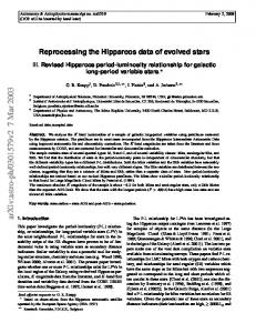
2 Symbolic representations are formal entities with which a perceptual system could make inferences about the abstract structures within a signal, such as surfaces in images or harmonic track sets in spectrograms [Milios and Nawab, 1989]. Consider in Figure 1.1 the example of the spectrogram, which is a discrete representation of the time-dependent frequency content of a signal. Specifically, it is a matrix of values indicating, for particular time regions of the signal, the coefficients (energy) for discrete sinusoid functions into which some frequencyanalysis algorithm has decomposed the signal. Examination of a three-dimensional view of the spectrogram shows that, over time, certain patterns in a signal’s frequency content can be discerned. The local maxima within the coefficients from a single time point represent “peaks,” or frequencies that are prominent in the signal at the given time. The regions within the spectrogram where a peak remains prominent over time form structures which are called tracks. The tracks can be modelled symbolically within a system as abstract structures with particular frequency variations, duration time durations, and energy variations, permitting the system to represent still “higher-level” structure such as observed relationships among the average frequency values of several tracks. A harmonic set, for example, is a set of tracks whose frequencies are integer multiples of some fundamental frequency f0.
"Track" f r e q "k" u e n c y
[ ]
s a m p l e s
v v ... v 1,k 2,k n,k . . . . . . . . . v v ... v 1,1
2,1
n,1
Energy Frequency
Time
"n" time points
Figure 1.1. Abstract “Tracks” in a Spectrogram.
Symbolic representations can serve as a basis for perceptual object models that impose top-down constraints on how a system processes a signal. For a basic example, consider
3 when a track is detected in a spectrogram (generated “bottom-up” from the spectrogram values). Symbolic sound-source models that list the frequency ranges in which a sound will generate tracks could limit (provide “top-down” constraints for) the time-frequency areas where additional tracking is done in the spectrogram to those within the track-regions of sounds containing the observed track.1 The presumed existence of one symbolic structure can also impose constraints on the nature of other structures to be searched for. An example of this occurs in the case of co-articulation phenomena in connected speech processing, where a phoneme at the end of one word can impose constraints on the acoustic characteristics to be expected at the beginning of the next word [Lee et al., 1990, Lowerre and Reddy, 1980]. Of course the decision to add interpretation processes to perceptual systems involved far more than the symbolic representations themselves. The inferencing processes that manipulate the representations, the control processes that schedule the inferencing and data-collection processes, and the data structures that organize data and the symbolic representations had to be built into the new perceptual systems as well. The body of knowledge to be incorporated in the software for perceptual systems would be quite complex. It was natural, therefore, for researchers to design software architectures that would provide "scaffolding" around which system code could be organized. Several architectures were developed from the mid-1970’s to the mid-1980’s, of which the most widely-used today is the blackboard architecture [Carver and Lesser, 1993a, Nii, 1986]. This architecture provides support for 1) a blackboard, or shared central storage data structure, that contains and organizes hypotheses about various signal features, 2) knowledge sources (KSs), or pieces of code each implementing expert knowledge about the relationships among signal hypotheses and the data that support them, and 3) a control component, or code that schedules the access of KSs to data and hypotheses stored on the blackboard, as well as the order of their execution. Since the early 1980’s, most perceptual architectures have incorporated the basic design shown in Figure 1.2. This design scheme produces systems with a numeric-oriented front end 1 As
discussed in Dorken’s thesis [Dorken 1994], the bottom-up generation of spectrogram tracks is a highly context-dependent problem.
4 that is logically separated from a symbolic-oriented interpretation component. The front end is permitted only one pass over the incoming signal, and the interpretation component is designed with the assumption that the front end’s output is always an "adequate" decomposition of the signal. Interpretation processes do not usually provide structured feedback to the front end about either the adequacy of the signal processing outputs to be interpreted or any anticipated signal behavior. The development of this scheme can be attributed to several factors, foremost among them being the influence of Marr’s reconstructionist school of thought in computer vision [Marr, 1982] and early psychophysical research on human perception which ignored the role of expectations in human interpretation of visual and auditory signals. Both influences led to the view that symbolic interpretation follows and depends upon signal decomposition by the front end through inversion of the geometry and physical processes that led to the original signal [Draper, 1993].
data correlates
signals
ENVIRONMENT
Front-End Signal Processing Algorithms
environmental interpretation
Interpretation Algorithms
Control Strategy + Object Models verification requests
Figure 1.2. Classic Signal Interpretation Architecture.
Within the blackboard paradigm, this design scheme resulted in a split at the control level between KSs that implement numeric signal processing algorithms (SPAs) and KSs that implement symbolic interpretation algorithms (SIAs).2 Control components generally pursue a strategy that first applies to the incoming signal a predetermined set of SPAs (the front end) with fixed control parameter values to obtain data correlates, or SPA outputs.3 The control 2 This
view, to be sure, is not the only one within the machine perception community. There is an alternative school of thought [Draper, 1993, Strat 1991, Kohl et al., 1987, Nagao and Matsuyama, 1980] that advocates feedback (in various degrees) between the front end and interpretation components of a signal interpretation system. As will be discussed in Chapter 3 the research in this thesis is complementary with this school. 3 Note
that the term “correlate” is taken from the voice-recognition literature. Within the signal processing
5 parameters of the SPAs are fixed to some setting that would provide correlates of adequate quality for generating hypotheses about symbolic structures. These correlates are then interpreted as reasonably certain support for symbolic signal structures at various abstraction levels. The control component uses these “islands of certainty” [Lesser et al., 1977] within the signal to index into an object-model database. The retrieved models then inform the control component in the application of additional interpretation algorithms to verify other signal structures that are required by the models. 1.2 Complex Environments and Traditional Design The traditional design paradigm assumes that a fixed front end can provide adequate (not necessarily optimal) evidence for reliable interpretations regardless of the range of possible scenarios in the environment. This assumption is plausible for systems that monitor stable environments, but not for those that monitor complex environments. In complex environments with interacting objects and variable signal-to-noise ratios, the choice of front-end SPAs and their parameter settings greatly impacts the generation of adequate correlates for interpretation processes.
Indeed, parameter values inappropriate to the current scenario can render a
perceptual system unable to interpret entire classes of environmental events correctly. An SPA’s parameter values induce capabilities or limitations with respect to the scenario being monitored. Consider the use of the generic Short-Time Fourier Transform (STFT) algorithm [Nawab and Quatieri, 1988] to produce spectrograms for acoustic signals. Conceptually, the algorithm implementing the STFT computes a series of Discrete Fourier Transforms (DFTs) [Oppenheim and Schafer, 1989] on successive blocks of data points in a discrete time signal. Referring to Figure 1.1, consecutive columns in the spectrogram matrix from an STFT are the DFTs of consecutive blocks of signal data. An STFT instance has particular values for its parameters: analysis window length (number of signal data points analyzed at a time), frequency-sampling rate (number of points computed per column in Figure 1.1’s matrix), and decimation interval (number of signal data points between consecutive analysis research community SPA outputs are referred to variously as “measurements,” “functionals,” or “statistics.”
6 window positions).4 Depending on assumptions about a scenario’s spectral features and their time-variant nature, these parameter values increase or decrease the usefulness of the spectrogram produced by the instance. It can be shown through analysis of Fourier theory (see [Oppenheim and Schafer, 1989], Section 11.3, for example) that a fixed STFT with a long analysis window length will provide fine frequency resolution for scenarios containing sounds with time-invariant components, but at the cost of poor time resolution for sounds with time-varying components. Tracks of sounds that change in frequency over time, or “chirp,” too quickly for the STFT will produce correlate peaks that look too widely separated to be linked as a track with a steep slope, while the onsets and decays of impulsive sounds will be “smeared” over the spectrogram, making it difficult to detect the presence of such sounds. Conversely, a fixed STFT instance with short window lengths will provide fine time resolution for scenarios containing sounds with time-varying components such as chirps or reverberatory decays, but at the cost of poor frequency resolution for sounds with close frequency components. The tracks of sounds which are too close to each other in frequency to be resolved (separated) by the STFT will produce correlate peaks that indicate only a single merged track in the output spectrogram. It should be noted at this point that analysis of the Uncertainty Principle [Gabor 1946] implies that one cannot obtain an STFT SPA instance (or, for that matter, design a new SPA) that simultaneously provides infinite frequency resolution and infinite time resolution. Figure 1.3 illustrates the difficulty in using fixed front ends to interpret a complex acoustic environment. Figure 1.3a shows the stylized frequency tracks of four sounds as they would appear in an ideal spectrogram if they were processed with STFT SPAs appropriate for each portion of the scenario. Darker shading indicates higher energy. Figure 1.3b shows how the tracks appear when the entire scenario is processed by one STFT SPA appropriate only 4 Note that this is a nonstandard usage of the term “decimation.”
The term “decimation” is most often used in the signal processing literature to refer to the process of first downsampling (reducing the number of sample values considered) a discrete signal and then lowpass filtering the result. (see [Oppenheim and Schafer, 1989], Section 3.6.1) There is no standard terminology for the STFT parameter being described here; “decimation interval” was selected because the parameter effectively controls how often windows of signal data are analyzed (i.e. how often the signal is “window-sampled”) to produce DFTs.
7 3760 Hz
Buzzer-Alarm 2540 Hz 2230 Hz
2350 Hz
Glass-Clink 1675 Hz
1475 Hz
950 Hz 500 Hz 460 Hz 420 Hz
Phone-Ring 1.0
Siren-Chirp 2.0
3.0
4.0 sec
1.0
2.0
TIME
TIME
(a)
(b)
3.0
4.0 sec
Figure 1.3. Example Problems From Fixed-Front-End Processing.
for the steady-state portion of the last sound (Siren-Chirp’s last 0.5 seconds) in the scenario. The STFT parameter settings used throughout Figure 1.3b were FFT-SIZE: 512, WINDOW: 256, and DECIMATION: 256, while the peak-picker’s parameter setting was PEAK-THRESHOLD: 0.09. The signal was sampled at 8KHz. DECIMATION is the separation between consecutive analysis window positions; the value was set to 512 to permit the fastest possible processing of the data. PEAK-THRESHOLD is the energy required for a Discrete Fourier Transform point to be considered as a peak, and its value here was selected to keep low-energy noise in the spectrogram from generating false-alarm tracks. Due to inappropriate processing, the analysis of the first two seconds of signal data introduces some distortions that would lead to ambiguous interpretations and completely undetected sources. A distortion is a process caused by poor SPA parameter settings that produces correlates that inaccurately represent the state of the environment to interpretation processes. In the first block of data (time 0.0 to 1.0 seconds) in Figure 1.3b, Phone-Ring’s tracks are merged because the frequency resolution afforded by the STFT is not adequate for features so close in frequency. Glass-Clink’s frequency track is not even detected in 1.3b’s next data block (time 1.0 to 2.0 seconds) because the STFT’s analysis window does not provide adequate time resolution to isolate the sound’s spectral features. The high peak-energy
8 threshold causes the peak-picker to miss low-energy peaks in the STFT spectrogram that could have served as evidence for Buzzer-Alarm’s high-frequency, low-energy track. Within the traditional design paradigm the approach to handling these types of problems is to add to the system’s front end more SPAs with settings appropriate to the problematic environmental scenarios. This requires an exhaustive analysis of the environment and intricate tailoring of front ends to each possible combination of perceptual objects in the environment. This approach is feasible only for significantly constrained environments. To avoid ambiguous signal-symbol mappings in complex environments, interpretation systems often require combinatorially explosive SPA sets with multiple parameter settings [Dorken et al., 1992], with consequent processing time costs. At this point one might question these criticisms of interpretation systems with fixed, one-pass front ends by claiming that the human auditory system, with its cochlear signal processing, is an example of a fixed, one-pass system that handles a wide variety of complex acoustic scenarios quite well. However, the claim misses (1) the fact that the human auditory system’s front end is only well-adapted for interpreting sounds from a moderately restricted environment that was evolutionarily important to the species, and (2) the possibility that two-pass revision, or reprocessing, occurs in the intermediate stages of the auditory system’s interpretation process. The cochlea’s time-frequency processing has been shown to be similar to that performed by wavelet analysis [Rioul and Vetterli, 1991] parameterized to produce spectrograms having fine frequency resolution with poor time resolution in the lower frequency regions, and poor frequency resolution with fine time resolution in the higher frequency regions. Thus, the human ear is able to discriminate low-frequency sounds (which, from an evolutionary standpoint, is useful for differentiating the growls and calls of predators or mates) and determine precise times for high-frequency events (which, from an evolutionary standpoint, is useful, for example, for localizing the position of stalking predators which may have snapped twigs or scrapped rocks). However, the fixed front end of this system creates difficulties for humans when they must handle scenarios from a more unrestricted environment. For example, the human ear’s poor
9 frequency resolution in the high-frequency spectral regions makes it ill-suited for discriminating among various aircraft engine whines that could indicate metal fatigue or poor balancing. Such unrestricted environments ultimately require additional “SPAs” (electronic hardware tuned to the particular engines) beyond those of the human ear for adequate interpretation, leading to the same type of combinatorial SPA explosion previously described. In regard to the second objection, Ellis [Ellis, 1996] summarizes work [McAdams, 1984, Warren, 1984] that indicates there is a possibility that the human auditory system reprocesses its initial interpretations. The McAdams work reported that during the initial presentation of an oboe note to human observers, a single note is perceived. However, as the note progresses, the even harmonics of the note undergo progressively deeper frequency modulation. This led observers to change their initial interpretation of the spectral energy as a single note to one in which there were two distinct sounds, and to apply that changed interpretation to the entire note. The Warren work examined how changes in the order of presentation of alternating wider (0-2KHz) and narrower (0-1KHz) noise-bands influenced the grouping humans performed on the signal components. When the narrower band came first, observers interpreted the signal as containing a continuous 0-1KHz sound with a periodic 1KHz-2KHz sound. That is, the lower 0-1KHz energy of the wider bands was merged over time with that of the narrower bands, as one might expect of a one-pass interpretation system that is primed to group new data with data that has just been observered. However, when the wider band started the alternation, observers reported that the first 0-2KHz band was interpreted as a single sound. After the initial wider band was completed, and as the alternation continued, however, the interpretation of the first band was revised to that obtained for the first alternation. That is, the observer reported that the first 0-2KHz band was perceptually “broken” into a 1KHz-2KHz burst simultaneous with a continuous narrower 0-1KHz sound, in light of the rest of the signal. Though by no means conclusive, both experiments lend support to the possibility that the human auditory system can revise its earlier interpretations.
10 1.3 Thesis Paradigm 1.3.1 Motivation To circumvent the combinatorial explosion of fixed SPAs, a small SPA set would be sufficient if comparisons could be made between the SPAs’ computed correlates and dynamicallygenerated signal structure expectations. Failure in the verification of expectations about SPA outputs can indicate that either 1) the signal structure expectations are based on incorrect interpretations or that 2) the SPA’s computed correlates have been distorted because the SPA’s parameter values are inappropriate to the current scenario. In the first case a perceptual system could follow the behavior of traditional interpretation systems and reinterpret the current scenario based on the SPA’s given correlates. In the second case a system could reconfigure the SPA’s parameters or selectively replace it with a more appropriate SPA, and reprocess the signal in a focused manner to obtain expected correlates. Adopting a search-oriented model of these two possible system responses to unmet expectations, one can see that the first behavior corresponds to a decision to evaluate how much better an alternative state in the interpretation state space might explain the front end’s output. The second behavior then translates into a decision to evaluate how much better an alternative state in the front end state space might be at generating evidence for unambiguously supporting an interpretation. Figure 1.4 shows how an interleaving of these behaviors results in progress in each search space. Figure 1.4A shows an interpretation system’s progress within its interpretation space. The label outside each state indicates the front end(s) being used to provide support evidence for the state’s interpretation (set of instances of perceptual objects Hn). Figure 1.4B shows the front ends explored by the system. The label outside each state indicates the interpretation expected for the front end, and whether the front end’s correlates supported the interpretation. The system behavior in Figure 1.4 can be summarized as follows. Initially, the interpretation system uses front end
A to collect evidence, and hypothesizes that one perceptual object of
type H1 is present. Attempting to account for more signal energy, the system then explores the
11 A
H1
SPA1(P1,P2) SPA2(Q1)
A A
H1 H3 SPA1(P1,P3) SPA1(P1,P2) SPA2(Q1)
H1 H1 H3 H1 H2 H3
A,B
Success! {H1} & {H1,H3} Failure! {H1,H2,H3}
H1 H3 H5
B
Failure! {H1,H2,H3}, {H1,H3,H5}, & {H1,H1,H3}
B,C
B SPA1(P1,P2) SPA3(P1)
H1 H1 H3 H4
C
C
Success! {H1,H1,H3} & {H1,H1,H3,H4}
B. FRONT-END SPACE
A. INTERPRETATION SPACE
Figure 1.4. Example of Dual Interpretation and Front-End Search.
f
g
interpretation state H1, H3 and finds that
A’s SPAs have also produced evidence to support
the interpretation. When attempting to explain the remaining signal energy, the system finds that an additional single object of either type H1, H2, or H5 could be hypothesized. Choosing
f
g
H2 first (i.e. the interpretation state H1,H2,H3 ), the system finds that the SPAs in front
A do not provide sufficient or unambiguous evidence for the H2 instance. Deciding that A is not suited for the interpretation, the system applies front end B ’s SPAs to the end
signal data, and this time finds negative evidence for H2’s instance, causing it to abandon
f
g
f
g
interpretation state H1,H2,H3 and proceed to explore H1,H3,H5 . The SPAs in front
B provided indisputable negative evidence for any instance of H5, leading the system to explore interpretation state fH1,H1,H3g. This time although B did not provide positive evidence for the second instance of type H1, the system finds that B was inappropriate to end
the interpretation. The system then uses signal processing constraints to determine that front end
C
should be appropriate for supporting or disproving the existence of the extra H1.
According to Figure 1.4B the correlates produced by the new front end do in fact support the second H1 hypothesis, and ultimately support the creation of a final H4 hypothesis. The final
f
g
interpretation state is H1,H1,H3,H4 , and because it accounts for enough signal energy, interpretation search stops. A domain’s explicitly-represented signal processing theory can play three generic roles in controlling the application of SPAs within constraints that dynamically arise from the emerging
12 list of observed symbolic structures: discrepancy detection: provide methods to determine discrepancies between an SPA’s expected correlate set and its computed correlate set. diagnosis: define distortion processes that explain how discrepancies between expectations and an SPA’s computed correlates result when the SPA has inappropriate values for specific parameters. reprocessing: specify new strategies to reprocess signals so that distortions are removed or ambiguous data is disambiguated. These observations about the power of formal signal processing theory in analyzing complex environments are the reasons behind the claim in this thesis that the explicit representation of the knowledge in signal processing theory is crucial to systems that monitor complex environments. The processing of signals from complex environments will benefit from a new view of signal interpretation as the product of two interacting search processes. The first search process involves the dynamic, context-dependent selection of signal features and interpretation hypotheses, and the second involves the dynamic, context-dependent selection of appropriate SPAs for extracting correlates to support the features. Signal interpretation architectures should support the use of theoretical relationships between SPA parameters and SPA outputs to structure these dual searches for SPAs appropriate to a scenario and for interpretations appropriate to the SPA correlates. 1.3.2 Architecture Overview This thesis proposes the Integrated Processing and Understanding of Signals (IPUS) architecture as a formal and domain-independent blackboard-based framework for structuring bidirectional SIA/SPA interaction in complex environments. This interaction combines the search for front end SPA configurations appropriate to the environment with the search for plausible interpretations of front end processing results. The architecture is instantiated by a
13 domain’s formal signal processing theory. It has four primary components as conceptual “hooks” for organizing and applying signal processing theory: discrepancy detection, discrepancy diagnosis, differential diagnosis, and signal reprocessing. These components have the following functionality:
� detect discrepancies between data expectations and actual data observations, � diagnose these discrepancies and ascribe reasons for observational uncertainty, � determine reprocessing strategies for uncertain data and expected scenario changes, based on the results of the diagnosis, and
� determine differential diagnosis strategies to disambiguate data with several alternative interpretations. To exploit the constraints that signal processing theory can impose on the dual searches within the signal interpretation problem, IPUS is designed with a “discrepancy detection, diagnosis, reprocessing loop.” The architecture uses an iterative process for converging to the appropriate SPAs and interpretations. For each block of data, the loop starts by processing the signal with an initial configuration of SPAs (KSs). These SPAs are selected not only to identify and track the signals most likely to occur in the environment, but also to provide indications of when less likely or unknown signals have occurred. In the next part of the loop, a discrepancy detection process tests for discrepancies between the correlates of each SPA in the current configuration and (1) the correlates of other SPAs in the configuration, (2) application-domain constraints, and (3) the correlates’ anticipated form based on high-level expectations. Opportunism in the architectural control mechanism permits this process to execute both after SPA output is generated and after interpretation problem solving hypotheses are generated. If discrepancies are detected, a diagnosis process attempts to explain them by mapping them to a sequence of qualitative distortion hypotheses. The loop ends with a signal reprocessing stage that proposes and executes a search plan to find a new front end (i.e., a set
14 of instantiated SPAs) to eliminate or reduce the hypothesized distortions. After the loop’s completion, if there are any similarly-rated competing top-level interpretations, a differential diagnosis process selects and executes a reprocessing plan to find correlates for features that will discriminate among the alternatives. Although the architecture requires the initial processing of data one block at a time, the loop’s diagnosis, reprocessing, and differential diagnosis components are not restricted to examining only the current block’s processing results. If the reprocessing results from the current block imply the possibility that earlier blocks were misinterpreted or inappropriately reprocessed, those components can be applied to the earlier blocks as well as the current blocks. Additionally, reprocessing strategies and discrepancy detection application-constraints tests can include the postponement of reprocessing or discrepancy declarations until specified conditions are met in the next data block(s). The dual searches discussed earlier become apparent in IPUS with the following two observations. First, each time signal data is reprocessed, whether for disambiguation or distortion elimination, a new state in the SPA instance search space is examined and tested for how well it eliminates or reduces distortions. Second, failure to remove a hypothesized distortion after a bounded search in the SPA instance space leads to a new search in the interpretation space. This happens because the diagnosis and reprocessing results represent an attempt to justify the assumption that the current interpretation is correct. When either diagnosis or reprocessing fails, there is a stronger likelihood that the current interpretation is not correct and a new search is required in the interpretation space. 1.4 Analysis of IPUS The IPUS architecture implements perception as the integration of search in a front-endSPA space with search in an interpretation space. This integration raises several issues, and encourages use of an alternative methodology for the design of perceptual systems’ front ends. This section briefly describes the major issues and introduces the real-world problem domain in which the thesis validates IPUS.
15 1.4.1 Architectural Implications The ability to interleave searches within the interpretation and front-end spaces raises the question of how one search process is determined to be the guide for the other, and how their roles can switch. In general, the search process whose current state produces the lower uncertainty serves as the standard against which progress toward a complete interpretation or adequate front end is measured in the other. Within the interpretation search process “uncertainty” refers to the portion of the signal5 explained by the current interpretation state and the strength of the negative (i.e. missing or incomplete) evidence against each hypothesis in the interpretation. Within the front-end search process “uncertainty” refers to the degree of inconsistency found among the data correlates from SPAs whose outputs are supposed to be related according to their domain signal processing theory. This reliance on uncertainty for driving and halting the dual searches in IPUS requires some mechanism for representing uncertainty; Chapter 2 details how the RESUN [Carver and Lesser, 1993b, Carver and Lesser, 1991] planning framework provides this mechanism. Another important question to consider about the interleaved searches is whether the interleaving process will converge. Although it is beyond the scope of this thesis to provide a formal convergence proof, the following line of reasoning serves as an informal indication that for a given finite subset of an input signal, convergence to a final interpretation hypothesis-set and a final front-end SPA-set will occur. With a given interpretation as a standard, IPUS might iterate on several diagnoses and reprocessings of a portion of the signal in attempts to verify particular missing data correlates required by the interpretation. With each iteration, correlates from various SPA-sequences with different control parameter settings will be generated. In the IPUS paradigm these correlates are said to have originated from different processing contexts. Assuming that not just each processing context but also their data correlates are recorded during reprocessing, the successive diagnose-then-reprocess iterations will generate tighter and 5 In
the IPUS framework evaluated in the thesis this will be the percent of the total input signal energy accounted for by the current interpretation.
16 tighter constraints on the types of signal features that could remain unobserved given all previous reprocessings. Eventually a point will be reached when the domain’s formal signal processing theory and the narrowing constraints on the possible values of an interpretation’s feature (e.g. track energy) preclude the existence of the desired data correlates. If search is restarted in the interpretation space, the results from previous reprocessings will constrain the new interpretation search by eliminating from consideration objects with features requiring correlates that should have been found during the reprocessing. As an IPUS-based system performs reprocessing, it will generate correlates from various processing contexts. Given the previous discussion’s conclusion that these correlates should be saved rather than discarded, the question arises as to how this data should be managed and exploited to offset its storage costs with time savings. As will be seen in Chapter 2, the explicit representation of processing contexts and the domain’s signal processing theory permits IPUS-based systems to examine their reprocessing history for processing contexts that would provide data correlates that were at least as detailed as those required by a current reprocessing request. If data correlates from such previous processing contexts exist, IPUS-based systems can save reprocessing effort by reusing them as evidence for missing evidence. This process is referred to as context mapping, and will be seen to be a useful mechanism for a type of sensor fusion where results from various reprocessings can be combined as evidence for time-dependent signal features. The final issue considered in this section involves the implications of the IPUS architecture for front-end design in interpretation systems. Since the traditional design paradigm has emphasized one pass over input signal data, there has been a tendency to build systems with fixed front ends that are expensive because they must provide detail for the most ambiguous cases even when the detail is unnecessary. Because IPUS has the ability to selectively reprocess uncertain portions of a signal with specialized SPAs, the framework provides many opportunities for using approximate processing techniques to reduce the complexity of front ends while sacrificing precision in SPA output where permissible. Approximate processing [Decker et al., 1990]
17 refers to the deliberate limitation of search processes in order to trade off certainty for reduced execution time. Approximate SPAs are algorithms whose processing time can be limited in order to trade off precision in their output correlates for reduced execution time. The availability of approximate SPAs permits the formulation of IPUS control strategies that first use approximate SPAs to generate a rough picture of the environment that is refined only where the front-end correlates’ interpretations are too uncertain. Refinement is achieved by reprocessing these limited signal portions with SPAs that produce correlates having greater precision. These non-approximate SPAs would ordinarily be quite expensive if applied to the entire signal, but when they are applied only in restricted signal regions their costs become manageable. 1.4.2 Architecture Validation Domain This thesis validates the IPUS architecture on the auditory scene analysis problem [Bregman 1990], which involves the segregation and identification of simultaneous and sequential sounds in an acoustic signal. Auditory scene analysis is an interesting problem that arises in applications such as assistive devices for the hearing impaired and robotic audition. The field is replete with issues concerning the relationship between the determination of an SPA’s appropriateness and multi-sound interactions in complex environments. In particular, the thesis work focuses on the problem of adaptively generating spectrograms that provide time- and frequencyresolution (i.e. detail in time or frequency) adequate to the task of separating signal signatures of simultaneous sounds with a variety of time-dependent behaviors. A secondary reason for performing validation in the acoustic domain is that signals from individual real-world sounds are relatively simpler to collect and easier to combine for experimental work than signals from other perceptual modalities such as vision or taction. All thesis evaluation experiments are performed on an IPUS-based Sound Understanding Testbed (SUT) implemented within the blackboard framework [Lesser et al., 1995, Lesser et al., 1993]. The system has 10 KSs implementing SPAs that can be used in front-end processing and 7 KSs implementing SIAs (signal interpretation algorithms) that generate high-level interpretations, as well as other KSs implementing the key components within the
18 IPUS architecture specification: discrepancy detection, discrepancy diagnosis, and differential diagnosis.
Table 1.1. IPUS Sound Library Categories CATEGORY chirp harmonic impulsive repetitive transient
PROPERTIES time-dependent frequency shifts sound has frequencies f1 ; : : : ; fn that are integer multiples of some fundamental f0 . short acoustic bursts cause wideband energy over entire frequency spectrum. need not have a precise period. signal onset or signal turn-off behaviors differ from those in steady-state.
EXAMPLES owl hoot, door creak fire alarm, car horn door knock, pistol shot footsteps, phone ring bell toll, hairdryer start
The testbed has a library of 40 real-world sound models from which to generate signal interpretations. The library sounds were selected to provide a reasonably complex subset of the acoustic behaviors and sound interactions that can arise in random real-world auditory scenarios. Table 1.1 summarizes the acoustic behaviors that can be found in the library. As an indication of the potential for interactions among sounds randomly selected from the library and placed in scenarios with random start times, it should be noted that the expected frequency range of each narrowband track (e.g.
� 100 Hz wide) of each library sound overlaps a track
of at least one other sound. Note that the greater the number of overlapping tracks there are in a spectral region, the greater the amount of interpretation search that must be done to disambiguate competing sound hypotheses that may arise. The IPUS performance experiments in this thesis are designed first to demonstrate in general the framework’s dexterity at effectively applying both special-purpose (e.g. approximate) SPAs and general-purpose (e.g. non-approximate) SPAs and adapting interpretations in complex scenarios and second to provide indications of the importance of the framework’s major “reprocessing loop” components to signal interpretation.
19 1.5 Contribution Summary To summarize, this thesis makes the following research contributions:
� a generic architecture for designing perceptual systems for complex environments that represents a significant departure from conventional systems,
� a framework for fusing correlates obtained from disparate front ends’ analysis, � through validation of the IPUS architecture in the real-world problem of auditory scene analysis: – a demonstration of the role of reprocessing and SPA theory in improving the quality of interpretations – a demonstration of the applicability and potential advantages of approximate processing within the IPUS architecture,
� a platform for future exploration of how to computationally approximate theories of auditory perception. 1.6 Thesis Organization The subsequent chapters in this thesis are organized as follows. Chapter 2 presents a detailed description of the IPUS architectural paradigm. Chapter 3 discusses work in signal interpretation architectures that is related to IPUS. Chapter 4 presents a description of how IPUS was instantiated in a sound understanding testbed (SUT). Chapter 5 reports on the SUT’s interpretation performance on acoustic scenarios composed of real-world sounds. Chapter 6 concludes with an evaluation of the SUT’s performance results and the IPUS framework’s organization, with respect to the research contributions outlined earlier. Appendix A supplies the interested reader with details on the sounds in the SUT library that was used in the experiment suites, while Appendix B contains a trace of the SUT’s behavior for one of the acoustic scenarios in Chapter 5’s experiments.
CHAPTER 2 INTEGRATED PROCESSING AND UNDERSTANDING OF SIGNALS This chapter presents the abstract, domain-independent specification for the IPUS architecture. It has five sections. The first section recounts an extended example of the basic behavior that this thesis aims for in a blackboard interpretation system for complex environments. With this description as a backdrop, the second section justifies and describes the RESUN planning framework that was selected to implement the architecture and provide appropriate control over blackboard KSs’ execution. The third section describes the RESUN implementation of the basic IPUS control strategy as well as the data structures and code that provide IPUS with the concepts of processing-context and adaptive front ends. The fourth section discusses the generic specifications of each component of the architecture’s reprocessing loop: discrepancy detection, discrepancy diagnosis, reprocessing, and differential diagnosis, including their abstract realization in the planning framework. The fifth section closes the chapter with a summary of what the architecture requires for instantiation. 2.1 IPUS-Based System Behavior: An Example In Section 1.2 the acoustic scenario in Figure 1.3 was used to illustrate the pitfalls of fixed front-end processing in complex environments. This section returns to that scenario for a concrete example of how an IPUS-based interpretation system with an initially inappropriate front end would ideally behave in processing a complex environment’s signal. Figure 2.1a shows the time-domain waveform for the signal, while Figures 2.1b and 2.1c duplicate the information from Figure 1.3 for the reader’s convenience. Figure 2.1b shows how the correlates for the sounds in the scenario would appear in the time-frequency domain using context-appropriate processing. Phone-Ring and Siren-Chirp are 1.2 times as energetic
21 as Buzzer-Alarm, and Glass-Clink is an impulsive source 3.0 times as energetic as Buzzer-Alarm. Darker shading indicates higher frequency-domain energy. Figure 2.1c shows how the sounds’ correlates are distorted when a front end reasonably designed for the end of the fourth data block is applied indiscriminately throughout the scenario.
Phone-Ring
Glass-Clink
Buzzer-Alarm
Siren-Chirp
2.5
2
1.5
1
0.5
0
-0.5
-1
-1.5
-2
-2.5
5000
10000
15000
20000
25000
30000
(a)
3760 Hz 2540 2230
Buzzer-Alarm 2350 Hz 1675 Hz
Glass-Clink
1475
500 460 420
Phone-Ring
950 Hz
Siren-Chirp 1.0 sec
2.0
3.0
4.0
3.0
4.0
(b)
1.0 sec
2.0
(c)
Figure 2.1. IPUS Processing Example.
Assume that an IPUS interpretation system has an STFT SPA, a local-peak-picker SPA, a time-domain energy-tracker SPA, and is configured to interpret the 8KHz-sampled waveform data in 1.0-second blocks. Assume also that the system’s sound-model database was loaded with models for the five narrowband sources shown in Figure 2.2. The vertical axis represents frequency and the horizontal axis represents time. The range below the time axis indicates the minimum and maximum expected durations for the sound’s spectral tracks. The energy changes for each track are represented qualitatively by shading gradations, with darker shades
22 indicating higher energy. In the figure the sounds’ frequency components are labelled by single-frequency values only for clarity; the formal sound definitions would have frequency ranges specified for each component.
3760 Hz 2540 Hz 500 Hz 460 Hz 420 Hz
1470 Hz [3.0, 5.0]
[1.6, 1.7]
Phone Ring Attack
Buzzer Alarm
Steady 2350 Hz
1950 Hz 1275 Hz
1675 Hz
730 Hz
950 Hz
440 Hz
550 Hz [1.3, 1.5]
[0.4, 2.5]
[0.4, 0.7]
Siren Chirp
Car Horn
2235 Hz
[0.10, 0.13]
Glass Clink
Figure 2.2. IPUS Processing Example’s Sound Database.
Next, assume that the front end SPAs were initialized with the following parameter values under the assumption that Siren-Chirp’s steady behavior (seen at the end of block 4) would predominate in the scenario: FFT-SIZE: 512 The number of uniformly-spaced frequency samples computed for each Short-Time Fourier Transform (STFT) analysis window position. WINDOW: 256
�
The number of data points to which each FFT in the STFT algorithm is applied ( FFT-SIZE).
23 DECIMATION: 256 The number of points between consecutive STFT analysis window positions. PEAK-THRESHOLD: 0.09 Spectrum points with energy below this value are rejected by the peak-picking algorithm. That is, assuming that Siren-Chirp’s steady frequency tracks are all separated by approximately 700 Hz, and that this kind of signal would predominate in the environment, the 31.25 Hz frequency resolution permitted by the length of the 256-point analysis window would enable the STFT to resolve the siren’s tracks with little difficulty. The decimation value of 256 is selected to ensure no overlap between consecutive analysis windows, which in turn provides the quickest complete processing of the signal data points, at a cost of interacting with the analysis window length to produce a spectrogram that can resolve frequency events no closer than 0.032 seconds in time. Lastly, the peak-threshold was selected to prevent the system from becoming distracted with noise-generated peaks whose energies are lower than that generally observed for Siren-Chirp’s steady tracks. Finally, assume that the system pursues an “island-driving” control strategy for each block where it executes the front end and produces peak hypotheses, then retrieves the models of sounds whose tracks roughly overlap the frequency regions covered by the peaks, then confirms the models’ tracks by verifying that the peak bounds unambiguously lie within the tracks’ expected regions. There are several critical behaviors that the IPUS system should perform if it is to reasonably analyze Figure 2.1a’s signal. In block 1, after initial front-end processing and model-retrieval, the system finds three alternative interpretations of the data in the [420; 500] frequency region. That is, there is the possibility that it could be caused by Phone-Ring or Car-Horn, or perhaps both occurring simultaneously. One reason for this confusion stems from the fact that the energy threshold setting for the peak-picking algorithm is high and would prevent Car-Horn’s low-energy microstream from being detected if in fact it were present. The second reason is that the frequency-sampling provided by the STFT algorithm’s fft-size parameter does not provide
24 enough frequency sample points to resolve the
;
[420 500]
region into Phone-Ring’s three
microstreams.1 The uncertainty in this situation should be resolved through reprocessing under the direction of differential diagnostic reasoning, which increases resolution and decreases the energy threshold. While verifying that the data in block 1’s supports all of Buzzer-Alarm’s tracks, the system also should detect that the sound’s track at 3760 Hz is missing. After engaging in signal processing diagnosis of the discrepancy, the system should find that one reason for this is that the track’s energy might be too low for the peak-picker’s peak-threshold parameter setting. The discrepancy would be resolved when the system reprocessed the existing spectrogram with a peak-picker having a lower peak-threshold value. In block 2, as it executes its front end, the system should detect a discrepancy between the outputs of its time-domain energy estimator SPA and its STFT SPA. Due to Glass-Clink’s presence, the energy tracking SPA’s correlates will indicate a substantial energy increase followed about 0.1 seconds later by a precipitous decrease. The STFT SPA, however, will produce a spectrogram with only one or two high-energy peaks, which, in a noisy environment, is not significant enough for believing that new short frequency track accounting for the time-domain energy flux is present at 2235 Hz. The system should determine through diagnosis that this could be because the STFT’s decimation value is too long. The testbed also detects a discrepancy between expectations established from block 1 for the [420; 500] frequency region and the STFT SPA’s output. The STFT SPA produces short contours that cannot support the expected microstreams for Phone-Ring because of inadequate frequency sampling in the region. Both discrepancies are resolved by reprocessing. The first discrepancy is resolved through reprocessing with a smaller decimation value and smaller STFT intervals, while the second is resolved through reprocessing with the finer frequency sampling provided by a 1024 fft-size. 1 Although the center frequencies of each track are further apart than the 8000=512 = 16:25 Hz frequency sampling afforded by the STFT, the tracks’ expected frequency ranges are too close.
25 In block 3, Siren-Chirp’s attack interacts with the poor time-resolution of the STFT SPA to produce a set of widely-separated peaks that the testbed cannot immediately interpret as the sound’s attack region. In block 4, however, the testbed should use the discovery of Siren-Chirp’s steady region as the basis for looking back to block 3’s region for the attack. After finding no conclusive peak support for the sound’s attack region, the system should diagnose the discrepancy as being attributable to poor time resolution in the spectrogram. It should then reprocess the waveform in the time-region of the expected chirp with an STFT suitable for detecting the behavior (e.g. one with a short WINDOW around 64 points long). 2.2 Control in IPUS From the preceding description of desired IPUS behavior, one should be struck by the important role the concept of “discrepancy” plays in how the architecture controls the application of SPAs and other KSs. It would appear useful therefore to design IPUS with the ability to represent discrepancies as symbolic, explicit factors that can influence the confidence levels a system maintains for interpretation hypotheses or numeric SPA outputs. Such sources of uncertainty (SOUs) could provide some of the cues for a control mechanism to use in making context-sensitive decisions to engage or interrupt the architecture’s reprocessing loop or dynamically modify a system’s default front end. Indeed, the overall context-sensitive nature of the hypothetical system’s behavior is a key feature. Though the hypothesized system required that the signal be processed one block at a time, the diagnosis, reprocessing, and differential diagnosis components were not restricted to examining only the current block’s processing results. When the current block’s processing results implied the possibility that earlier blocks were misinterpreted or inappropriately reprocessed, those components were applied to the earlier blocks as well as the current blocks. Although it did not happen in the example scenario, the postponement of reprocessing until specified conditions are met would also be a useful context-sensitive behavior for cases when uncertain signal data at the very end of a block requires the next block’s data for meaningful reprocessing.
26 For these reasons, IPUS uses Carver’s RESUN [Carver and Lesser, 1993b] planner framework to control blackboard KS execution. This framework views interpretation as a process of gathering evidence to resolve hypotheses’ SOUs. It incorporates a rich language for representing SOUs as structures which trigger the selection of appropriate interpretation strategies. For some idea of the this representation’s scope, consider the following partial list of SOUs in the language. There is an SOU called Partial-Support, which, when found on a blackboard hypothesis, represents the situation that the hypothesis has uncertainty because support evidence has not yet been sought for it (e.g. a spectrogram track’s termination has not been searched for yet). Another SOU called Possible-Alternative-Explanation represents the situation that a hypothesis is uncertain because there exist other explanations for it that have not yet been considered. A third SOU called Support-Exclusion represents the uncertainty that a hypothesis has because some subset of the support evidence desired for it has not been found because it is highly likely that the evidence in fact does not exist. In addition to its SOU language, the RESUN planning framework provides an elaborate language for specifying and executing the plans available to a system for satisfying the goals it generates as it solves an interpretation problem. The following brief description of the controlplan framework concentrates on the RESUN features that are relevant to IPUS; interested readers can find more detailed treatments in the planning community’s literature [Carver and Lesser, 1993b, Carver and Lesser, 1991]. Problem-solving under RESUN is driven by information in a problem solving model (PSM), which is a data structure that maintains a list of the current highlevel blackboard interpretation hypotheses and the SOUs associated with each one’s supporting hypotheses. SOUs from the PSM are selected by the planner to be resolved. That is, with selection of an SOU, the RESUN planner establishes a goal that the SOU be eliminated or reduced, if possible. Goals are expressed as predicate statements such as (Have-SOU-Solved *SOU*) where *SOU* would be an SOU to be solved. The planner controls the selection and execution of blackboard KSs for achieving this goal with its library of control plans and focusing heuristics. Both Figures 2.3 and 2.4 should be consulted closely
27 in the following discussion of control-plan definitions, while Figure 2.3 should aid in the later discussion of focusing heuristics.
Root-Plan GOAL: ROOT IN: ?A, ?B INTERNAL: ?C, ?D OUT: ?E
SEQ
Subgoal-2 IN: FOCUS(?C) OUT: ?X
Plan
Plan
Matching
IN: ?A, ?B OUT: ?C
Matching
Subgoal-1
Subgoal-3 IN: ?A, ?X OUT: ?E
FOCUS(match-list)
Primitive-X
Plan-9
Plan-1
GOAL: Subgoal-1 IN: ?IN1, ?IN2 OUT: ?OUT1*
GOAL: Subgoal-2 IN: ?IN1 INTERNAL: OUT: ?OUT1
GOAL: Subgoal-3 IN: ?IN1, ?IN2 INTERNAL: ?X, ?Y, ?Z OUT: ?OUT1
Figure 2.3. Control Plan and Focusing Heuristics.
A control plan is a plan schema that specifies either a set of subgoals that must be met in order achieve the plan’s goal, or a primitive action (e.g. blackboard KS or other code for manipulating objects on the blackboard or planner’s data structures) that can be taken immediately to achieve the plan’s goal. As shown in Figure 2.3, a control plan’s definition includes a GOAL form indicating the predicate form of the goal that the plan is intended to satisfy. The RESUN planner uses this information to retrieve any relevant plan from its plan library, then logically unify the goal form with the plan’s goal form and variables. IN and OUT plan variables are used to pass information to higher-level plans, while INTERNAL variables are used to pass information among a plan’s subgoals. RESUN’s subgoal grammar supports the specification of rather complex scheduling relationships and dependencies among the subgoals of a plan. To aid the reader in understanding the structure of IPUS control plans, Figure 2.4 illustrates the five common subgoal relationships used in plans for IPUS:
28 (A) Subgoals must be achieved in sequential order left-to-right. (B) Subgoal-1 must first be achieved, then depending on the value returned by g(), either subgoal-2 (g (?C ) = 0) or subgoal-3 (g (?C ) = 1) must be achieved. (C) Subgoal-1 and subgoal-2 both must be achieved, but in any order. (D) Subgoal-2 needs to be achieved only if the condition is true. (E) Subgoal-2 must be repeatedly achieved until the condition is false.
Root-Plan
Root-Plan GOAL: ROOT IN: ?A,?B INTERNAL: ?C OUT: ?D
GOAL: ROOT IN: ?A, ?B INTERNAL: ?C OUT: ?D
SEQ
SEQ XOR(g(?C))
Subgoal-1
Subgoal-2
Subgoal-1
Subgoal-2
Subgoal-3
IN: ?A OUT: ?C
IN: ?B, ?C OUT: ?D
IN: ?A OUT: ?C
IN: ?A, ?B OUT: ?D
IN: ?B, ?C OUT: ?D
(A)
(B)
Root-Plan
Root-Plan
GOAL: ROOT IN: ?A,?B INTERNAL: OUT: ?C
GOAL: ROOT IN: ?A, ?B INTERNAL: ?C OUT: ?D
SEQ
SHUFFLE
COND(?C = NIL) Subgoal-1
Subgoal-2
IN: ?A OUT: ?C
IN: ?B OUT:
Subgoal-1
Subgoal-2
Subgoal-3
IN: ?A OUT: ?C
IN: ?A, ?B OUT: ?C
IN: ?A, ?C OUT: ?D
(C)
(D) Root-Plan GOAL: ROOT IN: ?A,?B INTERNAL: ?C, ?X OUT: ?D
SEQ ITER(?X > 100) Subgoal-1
Subgoal-2
Subgoal-3
IN: ?A OUT: ?C
IN: ?B, ?C OUT: ?X
IN: ?A, ?X OUT: ?D
(E)
Figure 2.4. RESUN Subgoal Relationships
Focusing heuristics are context-sensitive tests for making a choice when there is more than one way to refine a plan. Figure 2.3 shows the two types of focusing heuristics used in IPUS:
29 variable-focusing heuristics and match-focusing heuristics. To see the role of variable-focusing, note that Primitive-X returns an uncertain value (?OUT1) which means that Subgoal-1’s ?C variable could have two or more possible values. A variable-focusing heuristic is applied to uncertain-valued variables when an attempt is made to use them in another subgoal (Subgoal-2 in Figure 2.3’s case). To see the role of match heuristics, note that Plan-1 was not the only plan in the control-plan database that could possibly satisfy Subgoal-3. A match-focusing heuristic, however, selected Plan-1. In both types of focusing, the decision is not final; if a subgoal could not be achieved with the first result of a focusing heuristic, the planner can (if the user so specifies) re-apply the heuristic to obtain the next best choice. Most significantly for IPUS, RESUN is an incremental planner, which means that plans are only expanded into constituent subgoals until the next primitive action that can be executed is identified. The action is then executed, and its effects on the blackboard or its output plan-variable results are used to update planner structures before more planning is performed. This has the important consequence of interleaving planning and KS execution, which in turn makes possible the kind of context-dependent behavior the thesis seeks for IPUS. The RESUN framework was developed to address existing interpretation systems’ limited ability to express and react to the reasons for interpretation hypotheses’ uncertainty. It emphasizes the separation of hypothesis belief evaluation from control decision evaluation by making control responsive not only to the levels of numeric belief in hypotheses but also to the presence of specific SOUs in the problem-solving model or on hypotheses. The refocusing formalism supports opportunistic control by enabling the planner to switch among several plan elaboration points (current leaf nodes in the plan tree) in a context-dependent manner. RESUN facilitates two basic problem-solving modes: evidence aggregation and differential diagnosis. Problem-solving for evidence aggregation seeks data for increasing or decreasing the certainty of one particular interpretation, whereas problem-solving for differential diagnosis seeks data for resolving ambiguities (uncertainties) that produced competing interpretations. IPUS-based systems need to use both problem-solving approaches in deciding when to reprocess
30 data previously examined under one SPA with another SPA to obtain evidence for resolving uncertainties. 2.3 Generic Architectural Strategy The generic IPUS architecture, with its primary data and control flow, appears in Figure 2.5. Solid arrow lines indicate dataflow relations. Dotted arrow lines indicate classes of plans that the planner can pursue when trying to reduce or eliminate particular uncertainties (discrepancies) in the problem solving model that were selected by the focusing heuristics. Note that the figure shows reprocessing being done only on the lowest-level SPAs for clarity’s sake. Within IPUS, reprocessing can cause SPA execution at any SPA output level, not just the lowest. Two types of signal interpretation hypotheses are stored on the hierarchical blackboard: interpretations of correlates from current and past signal analyses, and expectations about the interpretations of data correlates from future analyses.
SOU summary
SOU selected by focusing heuristics Problem Solving Model
{
Control Planner
hypotheses expectations Level N . . .
(Interpretation KSs)
hypotheses expectations Level k+1 SPA output Level k+1 . . . SPA output Level 1
{
Blackboard
Selected Control Plan: one of Interpretation KSs, Reprocessing Loop, Differential Diagnosis, or SPA execution
(SPA KSs)
Discrepancy Detection
Differential Diagnosis
Diagnosis
Reprocessing
Reprocessing Loop
Signal Data
Figure 2.5. The Abstract IPUS Architecture
The IPUS architecture is designed to support variations on the following four-phase general control strategy. Within the first phase, each block of signal data is processed with an
31 initial configuration of SPAs (initial front end), producing data correlates at various blackboard abstraction levels up to some cutoff level. As the initial front end is executed, discrepancy detection tests are performed to check for discrepancies between each SPA’s data correlates and (1) the correlates of other SPAs in the configuration, and (2) application-domain constraints. Depending upon the system designer’s intentions, IPUS provides the ability either to proceed to the second phase of execution, to act immediately upon detected discrepancies at this point (third phase), or to interleave these behaviors. In the second control-strategy phase, IPUS applies signal interpretation algorithms (SIAs) to the front end results both to confirm support for expectations from previous data blocks’ interpretations and to generate new hypotheses to explain unexpected correlates’ occurences.2 In the course of confirming expected correlates, IPUS performs a third set of discrepancy-detection tests to compare the initial front end’s output with the correlates’ anticipated form based on high-level expectations. During the third general control phase IPUS selects various discrepancies, generates diagnostic explanations for them, and, if explanations exist, searches for and applies new front ends to eliminate or reduce the discrepancies. As before, IPUS permits a system designer to interleave actions from this phase with actions from the second phase. In the fourth and final control-strategy phase, if there are any similarly-rated competing top-level interpretations, IPUS can perform differential diagnosis to select and execute reprocessing plans to find correlates for features that will discriminate among the alternatives. At the end of this phase, IPUS also allows the system designer to specify methods for updating the initial front end for the next data block so as to prevent reprocessings for predictable discrepancies. 2.4 Basic IPUS Machinery This section describes both the RESUN elements and the IPUS-specific mechanisms that provide the framework for the general IPUS architecture. The first subsection describes the role of RESUN’s SOU concept in IPUS, while the second subsection presents the basic control 2 for example, new tracks from a newly-started
a camera’s field of view.
sound or a new shadow from an object that has just moved into
32 plans that implement IPUS. The third subsection concludes with a discussion of the IPUS mechanisms for supporting processing contexts and adaptable front ends. 2.4.1 SOUs and IPUS The key to using RESUN to implement the general IPUS control strategy yet provide generality for system designers using IPUS in various domains lies in RESUN’s SOU concept. It is the generality of the RESUN SOU language that gives IPUS its own generality. IPUS requires a system designer to specify control decision tests using both application-specific focusing heuristics and application-specific control plans. These tests must be expressed in terms of what kinds of SOUs are present in the PSM or on a particular hypothesis. There are three general categories of SOU that IPUS borrows from RESUN, which are named according to where SOUs in the category can be found within IPUS: 1. Problem-Solving-Model SOUs These SOUs are used to summarize the general state of the current interpretation. IPUS makes use of four RESUN SOUs in this category: (a) No-Evidence: Summarizes where the current interpretation is uncertain because there is unprocessed signal data beyond the current data block. (b) Uncertain-Hypothesis: Summarizes which hypotheses in the current interpretation are uncertain and why. This SOU is used with symbolic interpretation hypotheses that are not at the “answer” blackboard abstraction level (the level of hypotheses at which a system is supposed to return results). (c) Uncertain-Answer: This SOU is used with symbolic interpretation hypotheses that are at the “answer” blackboard abstraction level, and that have sufficient (though possibly incomplete) support to be believed. Summarizes which believed answer-level hypotheses are uncertain and why. (d) Uncertain-Nonanswer: This SOU is used with symbolic interpretation hypotheses that are at the “answer” blackboard abstraction level, and that have sufficient
33 (though possibly inaccurate) negative evidence to be disbelieved. Summarizes which disbelieved answer-level hypotheses are uncertain and why. 2. Hypothesis SOUs These SOUs are used to express general reasons for why a particular hypothesis is uncertain. IPUS adopts eight from the RESUN SOU language, and uses a ninth SOU specific to the architecture: (a) No-Support: This SOU represents the uncertainty in a hypothesis that arises because it was generated through top-down inferencing and not any support hypotheses have yet been sought for it. (b) No-Explanation: This SOU represents the uncertainty in a hypothesis that arises because no bottom-up inferencing has yet been done to explain it as a feature of (i.e. evidence for) a higher-level hypothesis. (c) Partial-Support: This SOU represents the uncertainty in a hypothesis that arises because not all of the potentially available support evidence for it has been searched for. (d) Support-Exclusion: This SOU represents the uncertainty in a hypothesis that arises because some subset of its required support evidence has been sought for but not found, which raises the possibility that the evidence may not in fact exist (e) Possible-Alternative-Explanation: This SOU represents the uncertainty in a hypothesis that arises because there exist explanations for it that have not been considered due to pruning decisions in the interpretation search space. (f) Possible-Alternative-Support: This SOU represents the uncertainty in a hypothesis that arises because there exist other classes of support that have not been considered due to pruning decisions in the interpretation search space or the front-end search space. (g) Alternative-Extension: Within RESUN (and IPUS), to represent the fact that a hypothesis at one abstraction level is supported by one or more other hypotheses at
34 lower abstraction levels, inference structures that link the hypotheses’ data structures are created. When the inference structure is created, copies of the involved hypotheses’ data structures are also created with updated attribute values according to the constraints of the inference. These copies are called hypothesis extensions. The alternative extension SOU represents the uncertainty in a hypothesis that arises because it has two or more extensions that support higher-level competing hypotheses. (h) Uncertain-Support: This SOU summarizes the uncertainty that a hypothesis has due to the uncertainty in the support hypotheses upon which it depends. Within IPUS this SOU serves as a “placeholder” in which focusing heuristics can find summary information about the uncertainty in the support for a hypothesis. (i) Constraint-Inconsistency: This SOU defined for IPUS represents the uncertainty in a hypothesis that arises because one or more domain-dependent relationships between it and other hypotheses have not been observed. For example, assume that the local maxima selected by a peak-picking SPA from a spectrum hypothesis must account for 50% of the spectral energy. If this constraint is not met, the spectrum hypothesis will be annotated with a constraint-inconsistency SOU. 3. Inference SOUs IPUS includes two SOUs in this category for representing uncertainty about the validity of inferences between support hypotheses and conclusion hypotheses. (a) Constraint: Occasionally some constraint in the application-rule that permits a support inference to be made is “moderately” violated. For example, assume a domain-specific rule that states that a set of frequency tracks in a spectrogram can be considered to represent (i.e. provide support for) a harmonic set if they are all integer multiples of a fundamental frequency. Depending on the application domain’s processing requirements, this rule might be considered to have been “moderately” violated when a set of tracks is used as support for a harmonic
35 set even though their frequencies each are 5 to 10 percent off from true integer multiples. Constraint SOUs represent the uncertainty in the inference caused by such situations. (b) Possible-Inappropriate-Parameter: This SOU represents the uncertainty in a negative inference that support hypotheses might be missing or distorted due to signal processing with an inappropriate front end, rather than because the support is not present. For example, an inference recording that no spectral peaks were found for an expected track hypothesis would be annotated with this SOU if the track’s possible range of expected energy included values below an energy threshold parameter used by the peak-picking SPA for identifying spectrogram values as peaks. 2.4.2 Basic IPUS Control Plans Figure 2.6 depicts the control-plans used to implement the most general control in IPUS: PSM-based control. After an IPUS system is initialized, it will iterate within the Resolve-PSM-Uncertainty plan until some iteration’s achievement of the HavePSM-SOU-Resolved subgoal results in the absence of a No-Evidence SOU in the PSM. In instantiating IPUS, the user must specify a variable focusing heuristic function for selecting the value of ?psm-sou from all sous in the PSM. Once a value is established, predefined match focusing heuristics based on the type of PSM SOU selected select a plan from those in Figures 2.7 through 2.11. The “No Evidence” control plan (Figure 2.7) effectively implements the first controlstrategy phase as well as the end of the fourth control-strategy phase defined earlier in this section. The “Uncertain Hypothesis” control plan and the “Uncertain Answer” control plan (Figures 2.8 and 2.9) will be seen to provide the hooks for users to add control plans implementing the remaining control-strategy phases. The “Uncertain Nonanswer” control plan (Figure 2.10) is provided as a hook for adding control plans that can re-evaluate certain disbelieved answer hypotheses when (for example) new signal data becomes available, while the “Solve PSM
36 Solve-Interpretation-Problem GOAL: ROOT IN: ?ps-criteria, ?library, ?init-front-end INTERNAL: OUT: ?answers
SEQ
Have-Initialized-System
Have-Interpretation-Uncertainty-Resolved
Plan
Matching
IN: ?ps-criteria OUT:
Plan
Matching
IN: ?ps-criteria, ?library, ?init-front-end OUT:
Resolve-PSM-Uncertainty
Initialize-System GOAL: Have-Initialized-System IN: ?ps-criteria, ?library, ?init-front-end INTERNAL: OUT:
GOAL: Have-Interpretation-Uncertainty-Resolved IN: ?ps-criteria INTERNAL: ?psm-sou, ?result, ?prev-sous OUT:
ITER (More data blocks exist) SEQ
Have-PSM-SOU
Have-PSM-SOU-Resolved IN: ?ps-criteria, FOCUS(?psm-sou) OUT: ?result
Plan
Matching
IN: ?ps-criteria, ?prev-sous OUT: ?psm-sou*
Get-PSM-SOUs GOAL: Have-PSM-SOU IN: ?ps-criteria, ?prev-attempts INTERNAL: OUT: ?sou
FOCUS(match-list)
?
Figure 2.6. Highest-Level IPUS Control Plans.
SOU List” control plan (Figure 2.11) is provided so that the system designer is free to have the PSM-SOU focusing heuristic return more than one SOU to be handled simultaneously. The ?ps-criteria input variable for these four plans is a means for making available a datastructure capturing high-level problem-solving constraints that govern the long-term behavior of a system, such as minimum required rating values for determining if a hypothesis is believed, or names of critical answer-level hypotheses that should be considered before all others. Such problem-solving criteria could have been incorporated in focusing heuristics, but they would then be static and unalterable for the duration of the system’s execution. Maintaining them in a modifiable data structure allows system designers to specify control-plans that could modify these constraints if the system’s environment changed from what it was when then system was originally deployed. At this point it is instructive to examine how the PSM-level control plans produce the general processing-strategy stages identified in Section 2.3. The discussion will first focus
37
Solve-No-Evidence-SOU GOAL: Have-PSM-SOU-Resolved IN: ?ps-criteria, ?psm-sou INTERNAL: ?region, ?front-end, ?waveform OUT: ?status
SEQ
Have-Earlier-Block-Pruned
Have-New-Data-Block
IN: ?psm-sou, ?front-end OUT:
IN: ?psm-sou OUT: ?waveform,?status
COND(?waveform) SEQ
Have-Updated-Front-End IN: ?ps-criteria, ?front-end OUT: ?front-end
Have-Front-End-Applied IN: ?waveform, ?front-end OUT:
Figure 2.7. “No Evidence” Control Plan.
Resolve-Uncertain-Hypothesis-SOU GOAL: Have-PSM-SOU-Resolved IN: ?ps-criteria, ?psm-sou INTERNAL: ?hyp-extension OUT: ?status
SEQ XOR(if (= ?hyp-extension :NONE) 1 0) Have-Uncertain-Extension IN: ?psm-sou OUT: ?hyp-extension
Have-PSM-Hyp-Disbelieved IN: ?psm-sou OUT: ?status
Have-Uncertain-Extension-SOU-Resolved IN: ?ps-criteria, FOCUS(?hyp-extension) OUT: ?status
Figure 2.8. “Uncertain Hypothesis” Control Plan.
Resolve-Uncertain-Answer-SOU GOAL: Have-PSM-SOU-Resolved IN: ?ps-criteria, ?psm-sou INTERNAL: ?answer-extension OUT: ?status
SEQ
Have-Uncertain-Extension
Have-Uncertain-Extension-SOU-Resolved
IN: ?psm-sou OUT: ?answer-extension
IN: ?ps-criteria, FOCUS(?answer-extension) OUT: ?status
Figure 2.9. “Uncertain Answer” Control Plan.
38 on the “No Evidence” control plan. The Have-Earlier-Block-Pruned subgoal of the “No Evidence” control plan provides system designers with a hook for incorporating criteria and strategies for simplifying the current interpretation before the next data block is examined. The “Simplify Interpretation” control plan in Figure 2.12 provides a general strategy for achieving the subgoal. This plan can be customized through focusing heuristics and domain-dependent plans and primitives for its subgoals. The overall strategy shown in Figure 2.12 has five stages. The first stage is represented by the Have-Answer-Summary subgoal, and involves the summarization of the answer-level hypotheses for the most recent data block into three categories: viable, dropped, and suspended. Viable hypotheses are those answer-level hypotheses that are believed, while dropped hypotheses are those answer-level hypotheses that have been disbelieved, or “pruned” from the interpretation,
Resolve-Uncertain-Nonanswer-SOU GOAL: Have-PSM-SOU-Resolved IN: ?ps-criteria, ?psm-sou INTERNAL: ?answer-extension OUT: ?status
SEQ
Have-Uncertain-Extension
Have-Uncertain-Extension-SOU-Resolved
IN: ?psm-sou OUT: ?answer-extension
IN: ?ps-criteria, FOCUS(?answer-extension) OUT: ?status
Figure 2.10. “Uncertain Nonanswer” Control Plan. Resolve-PSM-SOU-List GOAL: Have-PSM-SOU-Resolved IN: ?ps-criteria, ?psm-sou-list INTERNAL: (as needed) OUT: ?status
SEQ
Have-SOU-Set-Handled IN: ?ps-criteria, ?psm-sou-list OUT: ?status
FOCUS(match-list)
Figure 2.11. “Solve PSM SOU List” Control Plan.
39 Simplify-Interpretation GOAL: Have-Earlier-Block-Pruned IN: ?no-evidence-sou, ?front-end INTERNAL: ?viable,?hyps, ?dropped, ?suspended, ?sufficientp, ?believed, ?disbelieved OUT:
SEQ
Have-Answer-Summary
Have-Answer-Sufficiency
IN: ?no-evidence-sou OUT: ?hyps, ?dropped, ?suspended
IN: ?viable, ?suspended, ?dropped, ?front-end OUT: ?sufficientp*
ITER(Unpruned competitors exist) ITER(and (not FOCUS(?sufficientp))
ITER(and (not FOCUS(?sufficientp))
?dropped))
Have-Competitors-Pruned
?suspended))
SEQ
SEQ
IN: ?hyps, ?viable OUT:?dropped
Have-Competitor-Reconsidered IN: ?hyps, ?no-evidence-sou, OUT: ?believed, ?disbelieved
Have-Nonanswer-Reconsidered IN: ?suspended, ?no-evidence-sou, ?viable OUT: ?suspended
Have-Answer-Sufficiency
Have-Answer-Sufficiency
IN: ?viable, ?suspended, ?dropped, ?front-end OUT: ?sufficientp*
IN: ?viable, ?suspended, ?dropped, ?front-end OUT: ?sufficientp*
Figure 2.12. “Simplify Interpretation” Control Plan.
in favor of a higher-rated competing hypothesis. Suspended hypotheses are those answer-level hypotheses that were disbelieved or eliminated from further consideration before all possible evidence for them had been sought because of a decision in some search-pruning focusing heuristic. The second stage is represented by the Have-Competitors-Pruned subgoal, and entails iteratively disbelieving hypotheses whose competitors have higher belief,3 until all lower-ranked competitors have been removed from consideration. The third stage is represented by the first Have-Answer-Sufficiency subgoal, which is achieved through a domain-specific focusing heuristic that determines the adequacy of the current data block’s interpretation (i.e. selects a true or false value for the ?sufficientp variable). “Adequacy” in this context refers to some set of domain-specific features that define the stopping criteria for problem-solving on a data block. When these criteria are met, the interpretation is assumed to be complete for the current data block, and the system can proceed to work on the next data block. The fourth and fifth “Simplify Interpretation” stages involve work on repairing interpretation inadequacies; their order can be switched according to application-domain requirements. In the iteration 3 The
belief metric can include tests for SOUs as well as numeric ratings.
40 that reconsiders dropped hypotheses, the first subgoal involves the determination of whether in fact a dropped hypothesis and its competitor are both present in the signal, in which case a pruning decision based on arbitrarily different ratings would be superseded. This subgoal can be achieved by the IPUS-supplied differential diagnosis control plan to be discussed in Subsection 2.5.4 or by domain-specific plans supplied by the system designer. In the iteration that reconsiders suspended hypotheses, the first subgoal involves the determination of whether in fact a suspended hypothesis had been discarded from consideration too soon, in which case a pruning decision based on an arbitrary rating at an arbitrary time would be superseded. This subgoal can be achieved by control plans whose subgoals require the IPUS-supplied “Uncertain Nonanswer” control plan in Figure 2.10 or by domain-specific plans supplied by the system designer. Continuing the elaboration of the subgoals of the PSM-level control plans, this subsection turns to the “Uncertain Hypothesis” and “Uncertain Answer” control plans, postponing discussion of the last two subgoals of the “No Evidence” plan to the next subsection. This is done since the material in Subsection 2.4.3 strongly interacts with the design of the plans for those subgoals. In general, the plan for uncertain-hypothesis PSM SOUs (Figure 2.8) leads to “bottom-up” system interpretation behavior or to diagnosis and reprocessing. That is, achievement of the plan’s subgoals involves either the explanation of hypotheses at lower abstraction levels as evidence for higher-level hypotheses, or the application of the reprocessing loop to resolve discrepancies noted among hypotheses produced by the front end. The first subgoal requires the selection of one extension when a hypothesis has more than one (Subsection 2.4.1, Alternative-Extension), and may involve focusing heuristics. The branch at the end of the plan permits the system designer to have the hypothesis disbelieved if no extension is found whose uncertainty can be resolved. This action might be justified, if, for example, the selection of an extension involved preliminary tests for whether the candidate extension could be used to hypothesize any higher-level or answer-level hypotheses. Failure to pass such a test could be an indication that the hypothesis represented a bottom-up derived “hallucination” that should be
41 disbelieved, or removed from further consideration by the interpretation processes.4 The second subgoal of the branch is handled by the short plan in Figure 2.13, whose subgoals require first the selection of some hypothesis SOU through a focusing heuristic, and second the resolution of the selected SOU. When a No-Explanation or Possible-Alternative-Explanation SOU is selected, domain-dependent control-plans are considered that will cause the problematic hypothesis to be explained as evidence for a higher-level or answer-level hypothesis. These “No Explanation” plans implement the part of the second general control-strategy phase that generates explanation hypotheses for unexpected hypotheses from SPA outputs, or generates preliminary answer-level explanations. When, however, a Constraint-Inconsistency SOU is selected, domain-dependent control-plans are considered that will perform discrepancy diagnosis and reprocessing for discrepancies detected in front-end results. These plans implement part of the third general IPUS control-stategy phase.
Resolve-Extension-SOU GOAL: Have-Uncertain-Extension-SOU-Resolved IN: ?ps-criteria, ?extension INTERNAL: ?ext-sou OUT: ?status
SEQ
Have-Extension-SOU
Have-Extension-SOU-Resolved
IN: ?extension OUT: ?ext-sou*
IN: ?ps-criteria, FOCUS(?ext-sou) OUT: ?status
Figure 2.13. “Resolve Extension SOU” Control Plan.
The “Uncertain Answer” PSM-level control-plan involves the achievement of subgoals analogous to those associated with the “Uncertain Hypothesis” plan, but the SOUs that it leads 4 Of
course, this conclusion is completely reasonable only if the system designer can assume that all possible types of hypotheses at the answer-level are known to the system (i.e. all possible perceptual objects are modelled in the system’s model library). When this assumption is not plausible, that is, there may be unknown objects whose structure (hypotheses below the answer-level) might be discerned but whose identity may be unknown, the system designer must exercise care in permitting consideration of the first XOR subgoal.
42 the planner to consider resolving on answer-level hypotheses or their supporting hypotheses are different. The planning associated with this plan’s subgoals will cause an IPUS system to resolve No-Support, Partial-Support, Possible-Alternative-Support, or Uncertain-Support SOUs indicating unsought support evidence at lower support-levels if focusing heuristics decide that the system should be engaged in the second part of the second phase of the general IPUS control stategy. That is, the system attempts to verify expectations from high-level interpretation hypotheses. Should focusing heuristics select Support-Exclusion, AlternativeExtension, or Uncertain-Support SOUs indicating low-quality support, domain-dependent plans implementing the remainder of the third general control strategy phase are considered. That is, planning is performed to apply the reprocessing loop to resolve discrepancies detected between interpretation expectations and front-end outputs. 2.4.3 IPUS and Front Ends This subsection discusses how SPAs are defined and embedded within an IPUS-based system and how the processing-context mechanism supports their manipulation. Before discussing the implementation of SPAs within IPUS, it is important to review the context-dependent nature of certain SPA executions. This review will serve as background for the reasons why various information categories about SPAs are included in IPUS. For the purposes of IPUS, the features that perceptual systems monitor in complex environments can be divided into two classes. The first class contains features which can be used to indicate the existence of one or more perceptual objects, though not necessarily the identities of those objects. These features often have supporting correlates that can be computed independent of the context being analyzed. In the auditory domain, for example, any collection of one or more “sound objects” may be conceptualized as an acoustic intensity distribution with minimum and maximum limits on gross features such as temporal spread, frequency spread, duration of silence intervals, and degree of randomness in intensity fluctuations. The SPA correlates for supporting such gross features can generally be computed in a context-independent manner; hence they are termed context-independent features.
43 The second feature class contains those features which can be used to identify an object or monitor the behavioral changes of an object. The computation of correlates to support these features is often very sensitive to the context being analyzed; hence they are termed context-dependent features in the IPUS design framework. In the auditory domain, for example, a frequency track would be a context-dependent feature of a sound (“acoustic object”). As Figure 2.14 illustrates, if the current interpretation for a scenario contains only one sound (sound A) having spectral energy at frequency f1, then even an STFT SPA with an analysis window length providing only very coarse frequency resolution (STFT-1, in addition to the other STFTs shown) would still produce correlates (a sequence of high-energy spectrogram values) that could support the claim that track TAf1 exists. However, as in Figure 2.15, an interpretation that assumes another sound (sound B) in the environment with spectral energy at a frequency f2 near f1 creates a new context with different processing needs. In this new scenario only STFTs providing frequency resolution of at least the minimum difference between f1 and f2 (STFT-3 only) will produce correlates that could unambiguously support the existence of
TAf1 (or, for that matter, the existence of TBf2 ). Figure 2.16 uses an instance of an environment suddenly changing from having one sound-source to having two sound-sources to provide a more concrete example of the context-dependent nature of track detection in a spectrogram in a real-world system. It is important to note that the distinction between context-independent and contextdependent features lies in the usage of the features. If a feature is used only to indicate the presence of some object(s), the feature is considered context-independent. However, if the same feature were to be used as support for the identity of some object(s), it would in general require context-dependent correlate computation, and would therefore be considered a context-dependent feature. Each time an SPA is executed within IPUS, the blackboard hypotheses representing the output correlates from the execution are annotated with the name of the SPA and the control parameter values used in the execution. This annotation is a data structure referred to as
44
STFT-3 256-pt window
Hz
TAf1
f1
time ASSUMED INPUT: Sound A with energy at the frequency f1
STFT-2 128-pt window
TAf1
Hz f1 time
STFT-1 64-pt window
TAf1
Hz f1 time
Figure 2.14. Context-Dependent Feature Example Part 1.
STFT-3 256-pt window ASSUMED INPUT: Sound A with energy at the frequency f1 plus Sound B with energy at the frequency f2
TAf1 TB f2
Hz f2f1 time
STFT-2 128-pt window
TAf1 TB f2
f1
Hz f2
time STFT-1 64-pt window
TAf1 TB f2
Hz f2f1 time
Figure 2.15. Context-Dependent Feature Example Part 2.
45 F r e q u e n c y
F r e q u e n c y
Time
Time
Source Tracks under Adequate Processing in Isolation Context A: Hairdryer alone
Context B: Hairdryer & Phone Rings
STFT-1: FFT SIZE: 256 ANALYSIS WINDOW: 128 DECIMATION: 64
STFT-2: FFT SIZE: 512 ANALYSIS WINDOW: 256 DECIMATION: 64
F r e q u e n c y
F r e q u e n c y
Time
( a )
F r e q u e n c y
Time
( b )
Time
( c )
Figure 2.16. Context-Dependent Example Part 3.
the correlates’ parameter context. In addition to the parameter context, each SPA correlate is annotated with a processing context, or a data structure listing the sequence of SPAs that produced the correlate from the input signal. In IPUS SPAs are defined with six elements. The first element is the actual code for the algorithm. The second element is the list of specific parameters that control how the algorithm produces output correlates, and bounds on the range of values each can take on. The third element is a set of rules defining how individual control parameters should be modified to eliminate or reduce various classes of distortions that could be manifested in the algorithm’s correlates. The preconditions of these rules are expressed in terms of one or more distortions, while the conclusions or actions of these rules specify methods for computing parameter values to ameliorate instances of the distortions. These rules actually are stored with reprocessing strategies. The concept of “distortion” is discussed further in Subsection 2.5.2. The fourth
46 element of an SPA definition is a set of discrepancy tests. These are application-dependent tests that compare the output of one SPA with the output of another SPA for consistency according to theoretical signal processing constraints. The fifth definition element is a list of “supercontext methods” that take as input a parameter-context and an optional “information category” label. These methods return patterns indicating the range of values for each control-parameter in an SPA parameter-context that would permit the SPA to produce correlates having the same or greater detail in the specified “information category” as found in the specified parameter context. The returned patterns5 must designate all SPAs which produce the same type of output as that produced by the SPA specified in the supplied parameter context, regardless of whether they share the same control-parameter sets. As an example, assume an SPA that selects local maxima from a spectrogram on the basis of whether their energy values are greater than a threshold control-parameter. The supercontext method for this SPA would, when supplied with a particular parameter context and the information category “peaks,” return a pattern indicating that any execution of the SPA with a parameter context having threshold values below that of the given parameter context would provide at least the same number of peaks as were produced by the given parameter context. The sixth and final SPA definition element is a mapping function that takes two parameter contexts and a list of correlates produced from the first context, and returns a list of the correlate hypotheses modified to reflect how they would appear had they been produced by the second context. Figure 2.17 shows the basic control plan used by IPUS for executing an SPA. The first subgoal, Have-Supercontext-Output, encourages the reuse of correlates from earlier SPA executions that could provide the same “information” as would be provided by the execution of the specified SPA with the parameter values specified in the ?context variable. This subgoal involves the application of supercontext tests. The ?context variable can hold either a parameter context, a processing context, or a front end, which is a list of parameter-contexts specifying the default control-parameter values to be used by the front end. In general, reuse occurs 5 In
the IPUS Sound Understanding Testbed these are simply parameter contexts with range-values for the control-parameters.
47 during reprocessing, and not during the first execution of the SPAs in the default front end. The second subgoal updates the region of application for the SPA based on what data was found that could be reused. The Have-SPA-Executed subgoal applies the SPA with the control-parameter values specified for it in the ?context variable. The final subgoal involves the application of discrepancy-detection tests for comparing outputs from the SPA for consistency with the outputs from other front-end SPAs or with environmental constraints.
Call-SPA GOAL: Have-SPA-Applied IN: ?input, ?region, ?spa ?context INTERNAL: ?new-regions,?old-results, ?new-input, ?new-results OUT: ?result
SEQ
Have-Supercontext-Output
Have-UpdatedRegions
IN: ?context, ?region OUT: ?temp-results
IN: ?old-results, ?region OUT: ?new-regions
Have-SPA-Executed IN: ?input, ?new-region, ?spa, ?context, ?result OUT: ?new-results, ?result
ITER(?new-regions) SEQ
Have-Discrepancy-Detection-Done IN: ?new-results, ?spa, ?context OUT:
Figure 2.17. “Call SPA” Control Plan.
The plan for executing the front end in IPUS is domain-dependent and must be specified by the system designer as a plan with COND clauses with calls to the Have-SPA-Applied subgoal. The COND test will check for whether the front-end SPA list contains a parameter-context with the name of the SPA the clause’s subgoal would cause to execute. The Have-Updated-Front-End subgoal of the Resolve-No-Evidence-SOU general IPUS control plan (Figure 2.7) involves the execution of rules for checking how often the current front end has caused diagnosable discrepancies and deciding whether a change in front-end SPAs or a change in SPA controlparameters is necessary to reduce the time spent in reprocessing. If changes are necessary, this subgoal will effect changes in the front-end SPA list.
48 2.5 IPUS Reprocessing Loop Components This section presents the generic specifications of each component of the IPUS reprocessing loop as depicted in Figure 2.5, and, where appropriate, describes the generic control-plan implementation for the component. 2.5.1 Discrepancy Detection The discrepancy detection process is crucial to the IPUS architecture’s iterative approach. The process is required to recognize three groups of discrepancies, based on the source of the expectation (i.e. ground truth) used in the comparisons. fault A discrepancy between an SPA’s computed correlates and correlates from other SPAs applied to the same signal data. This class is included based on two propositions. The first is that correlates for context-dependent features, if computed by SPAs appropriate to the context, do not contradict the correlates for context-independent features. The second is that correlates for context-dependent features, if computed by SPAs appropriate to the context, do not contradict other context-dependent correlates computed by other SPAs from the same data. Figure 2.18 illustrates this type of comparison with an acoustic example comparing the context-independent output of a time-domain energy-tracking SPA with the context-dependent selection of peak values from the output of an STFT SPA. The energy tracking SPA indicates a short burst of energy while the first STFT’s correlates do not support new frequency tracks during the burst’s time period. A fault should be declared in this case since Fourier theory requires indications of the burst’s presence in both analyses,6 given the assumption that the peak-picking analysis done on the STFT’s output was appropriate to the environment. violation A discrepancy detected between an SPA’s data correlates and domain constraints. This class is included based on the proposition that correlates, if computed by SPAs appropriate 6 Specifically,
X
N?1 Parseval’s Theorem
n=0
[ ]2=
jx n j
1 N
X
N?1 k=0
[ ] 2 requires that time-domain energy (lefthand
jX k j
side) be conserved in the frequency-domain (righthand side).
49 5000 Hz
Footstep+Noise
1.0
TIME
STFT-1: FFT SIZE: 2048 ANALYSIS WINDOW: 1024 DECIMATION: 128
STFT-2: FFT SIZE: 1024 ANALYSIS WINDOW: 256 DECIMATION: 32
Energy Tracking
5000 Hz
5000 Hz E n e r g y
TIME
1.0
TIME
1.0
TIME
1.0
Figure 2.18. Fault Discrepancy Example.
to the context, do not support features that violate the environment’s physical constraints. As an example, if the application domain is considered subject only to wideband gaussian noise (5000 Hz wide), STFT output correlates showing only a narrowband noise signal (say 500 Hz wide) would give rise to a violation. Note that violations can indicate either that an SPA was inappropriately applied or that the environment’s characteristics have changed from those in the assumed in the current interpretation. In the first case reprocessing based on the interpretation should succeed in eliminating the discrepancy. In the second case reprocessing based on the invalid interpretation should fail. conflict A discrepancy between an SPA’s computed correlates and model-based expectations. Model-based expectations arise from two sources. The first source is the set of models for objects already assumed to be present. The second source is the set of models for objects under consideration for interpreting newly-detected correlates in the current block of data. Conflict discrepancies may involve either a total or a partial mismatch
50 between correlates and the hypotheses they were supposed to support. This class is included based on the proposition that features supported by correlates computed from appropriate SPAs ought to be completely consistent with the object features specified by the context expected to be observed. The concept of “object features” includes not only features that are not expected to be distorted but also features that are expected to be distorted because of the existence of other objects in the environment. Conflicts can indicate that an SPA is not appropriate to the context or that the context actually contained objects different from those expected. As a simple example, a conflict would occur when the interpretations of past correlates predict a sound with two tracks at 230 Hz and at 250 Hz with no decline in their amplitudes, but peaks picked from the current spectrogram support only one or none of the tracks. This discrepancy could indicate that possibly the peak-picker’s energy threshold is inappropriate because the sound’s volume decreased, or that a new sound’s tracks are overwhelming those of the expected sound. Fault and violation discrepancies are tested for during the achievement of the HaveDiscrepancy-Detection-Done subgoal in the “Call SPA” control-plan of Figure 2.17. The tests for these discrepancies are application-dependent and are specified in the "discrepancy-test" element of each SPA’s definition. When discrepancies are found, they are represented as Constraint-Inconsistency SOUs on the problematic hypotheses. Conflict discrepancies are tested for within SIAs while they search for evidence confirming expectations. If no evidence is found, the conflict is represented as a Support-Exclusion SOU on the expectation hypothesis. When there is reason to believe that the lack of evidence could be attributable to use of an inappropriate front end,7 a Possible-Inappropriate-Parameter SOU is attached to the negative inference structure linking the unverified expectation hypothesis with an empty evidence set. On the other hand, if partially supportive evidence is found, the support inference structure between the expectation hypothesis and the support evidence is annotated with a Constraint 7 This determination should be limited to simple heuristic checks of SPA parameter values rather than complex tests involving deep SPA knowledge that would be performed only by the discrepancy diagnosis KS.
51 SOU. In general, it is the presence of inference SOUs that identifies the presence of conflicts that may be rectifiable by the reprocessing loop. In all cases the SOUs are annotated with the processing contexts used in the failed or partially successful attempts at finding desired evidence. Examination of a wide range of domains reveals two generic classes of correlates: point correlates and region correlates. A point correlate is a value associated with one point in the SPA output coordinate space. A region correlate is a value associated with a subset of the SPA output space. Consider the following examples. A spectral peak energy value in the “time, frequency, energy” space of acoustic signal processing and an image pixel intensity value in the “x, y, intensity” space of image processing are examples of point correlates. A noise-distribution tag for a region in a radar sweep and a mean-intensity value for a region in the output of an image filtering SPA are examples of region correlates. A track of spectral peaks over several time slices from a spectrogram is an example of a region correlate comprised of non-contiguous subsets of the SPAs’ output space. For both point and region correlates, the IPUS discrepancy detection component must support tests for the following generic discrepancies between an SPA’s anticipated correlate set and its computed correlate set. 1. missing: An anticipated correlate is not in the computed correlate set. An example of this discrepancy in the acoustic domain occurs when a spectral peak is expected in the output of an FFT SPA, but is not found. 2. unassociated: An unanticipated correlate occurs in the computed correlate set. An example of this discrepancy in the radar domain occurs when an unanticipated clutter region is produced during a radar sweep. 3. value-shift: A correlate is found in the computed correlate set at its anticipated coordinates, but with an unanticipated value. In the visual domain this discrepancy would be encountered when an image region’s hue label produced by a color-analysis SPA is different from the one expected.
52 4. coordinate-shift: A correlate with an anticipated value is found in the computed correlate set but at unanticipated coordinates. This includes the situation where a region’s boundaries shift from their expected locations. An example of this discrepancy in the acoustic domain occurs when a track of spectral peaks produced by a curve-fitting algorithm has the correct energy value but is 30 Hz from its expected position. 5. merge: Two or more anticipated correlates are deemed to have appeared as one unanticipated correlate in the computed correlate set. The criteria for this merging are domain-specific and often depend on relationships between the missing correlates’ values or coordinates and the unanticipated correlate’s value or coordinates. An example of this discrepancy in the visual domain occurs when two adjacent regions with different expected textures are replaced by one region with an unanticipated texture. 6. fragmentation: An anticipated correlate is deemed to have been replaced by several unanticipated correlates in the computed correlate set. The criteria for this splitting are domain-specific and often depend on relationships between the missing correlate’s values or coordinates and the unanticipated correlates’ values or coordinates. An example of this discrepancy in the radar domain occurs when a noise-analysis SPA computes two or more small regions with a particular noise-distribution label instead of an expected single region with that label. 2.5.2 Discrepancy Diagnosis SPA processing models serve as the basis for defining how the parameter settings of an SPA can introduce distortions into the SPA’s computed correlates. These distortions cause correlate discrepancies. Consider an SPA processing model rule relating the STFT’s WINDOW-LENGTH parameter to the characteristics of SPA output and how this model can be used to define distortions. Formally, Fourier theory defines the following relationship. Assume that an STFT with a rectangular analysis window of a discrete signal that has been sampled at
W
sample points is applied to
R samples per second.
If the signal came from
53 a scenario containing frequency tracks closer than
R=W
Hz, the correlates for those tracks
in the STFT’s spectrogram (values in the spectrogram matrix indicating prominent energy at the track frequencies over time) will be merged and will support at most one distinct track. Referring to Figure 2.16, as the WINDOW-LENGTH parameter’s value increases, merged and missing correlate discrepancies between (b) and the tracks expected from the updated interpretation disappear. Conversely, as the parameter’s value decreases, merged and missing correlate discrepancies occur more frequently. The primary formal task of an IPUS discrepancy diagnosis KS is to generate a sequence of distortions that can explain the discrepancies between an initial state that represents the assumed ground-truth (e.g. application-specific signal constraints, high-level expectations, or outputs from alternative SPAs whose outputs are less precise but more reliable) and a goal state that represents the observed SPA output. In effect the distortion list provides an “inverse mapping” explaining how the ground-truth could have been misrepresented by the front end so as to appear like the observed correlates. Note that there is a difference between discrepancies and signal distortion processes; there is not usually a one-to-one mapping between discrepancies and distortions. It is possible for several distortion processes to explain the same kinds of discrepancies. A “low frequency resolution” distortion explains the “missing” discrepancy in Figure 2.19’s example, but a “low time resolution” distortion would explain the “missing” discrepancy between the outputs from the first two SPAs back in Figure 2.18’s example. Within IPUS, the actual discrepancy-detection KS is considered domain-dependent, as is the implementation of the distortion knowledge. It will be seen in Chapter 4 that the Sound Understanding Testbed (SUT) used a discrepancy-detection KS that relied on means-ends analysis to generate a list of distortion operators that reduced the differences between an initial state representing the expected form of front-end data or the expected form of high-level interpretation hypotheses, and a final state that represented the observed data or hypotheses. However, a system designer using IPUS would be free to specify some other KS design, perhaps based on neural nets or cased-based reasoning.
54
Hz
T1 T2
Hz DISCREPANCY MISSING track correlates for T2
T1 T2???
Time
Time
What Was Actually Supported
Interpretation Expected
Distortion Definition Low Frequency Resolution Preconditions: N expected tracks present within a frequency region SAMPLE-RATE / WINDOW-LENGTH Hz wide. Result: Expect only one track having energy approximately equal to sum of N expected microstreams, and frequency-range equal to region in precondition.
Distortion Mapping (LOW-FREQUENCY-RESOLUTION)
Hz
Hz
DISTORTION LIST (explanation) Time INITIAL STATE (interpretation expected)
Time
FINAL STATE (interpretation that was actually supportable)
Figure 2.19. Sample Distortion Explanation.
The domain-independent input requirement for the KS is that it accept as input an SOU structure that will point to the hypotheses on which it is stored and that can contain a record of failed diagnosis explanations that did not enable the reprocessing component to resolve the SOU. The domain-independent output requirement for the KS is that it return an explanation structure containing a list of distortions, the processing goals for eliminating them, and the region in which diagnosis was performed. In principle the processing goals depend on the domain. However, in the development of the Sound Understanding Testbed reported in Chapter 4, only two general goals were found necessary. The first is of the form (Have-Hypothesis-Supported ?hyp), which is specified when the SOU under consideration is related to some hypothesis (?hyp) for which no support evidence was found, and the explanation requires that the hypothesis be supported. The second general processing goal is of the form (Have-Hypothesis-Characterized ?hyp ?feature). This goal is specified when the elimination of the distortions merely requires a more refined value for ?hyp’s feature named in ?feature, or
55 the calculation of the feature if it hadn’t already been calculated. The SOU being diagnosed is annotated with the explanation structure, permitting the IPUS planner the flexibility of postponing reprocessing for the SOU in case a PSM SOU unrelated to the diagnosed SOU demands attention. 2.5.3 Reprocessing The signal reprocessing component of IPUS uses explanations from the diagnosis components to propose and execute search plans for finding new SPA control parameter values that eliminate or reduce the hypothesized distortions. In the course of a reprocessing plan’s execution, the signal data may be reprocessed several times under different SPAs with different parameter values. The incremental search is necessary because the diagnosis explanation is at least partially qualitative, and therefore it is generally impossible to predict a priori exact parameter values to be used in the reprocessing. The reprocessing component relies on user-encoded knowledge from SPA processing models to select new SPAs and/or parameter values when instantiating the proposed reprocessing plan. The input to the general reprocessing control-plan is the diagnostic explanation for resolving an SOU. Strategies for eliminating various distortions are specified as domain-dependent control plans to be selected by the IPUS planner as indexed by the diagnostic explanation. From the retrieved set of applicable plans, one is selected by domain-dependent focusing heuristics. Selections can be governed by criteria such as estimated plan execution time, or the availability of data from earlier executions of SPAs that were supercontexts of SPAs to be executed. The execution of a reprocessing plan consists of incrementally adjusting the control parameters of SPAs within the plan, applying the SPA sequence to the portion of the signal data that is hypothesized to contain distortions, and testing for discrepancy removal. The incremental process is necessary because the situation description is at least partially qualitative, and therefore it is not generally possible to predict exact values for the control parameters to be used in the reprocessing.
56 Reprocessing continues until the goal of distortion removal is achieved or it is concluded that the reprocessing plan has failed. There are two general criteria for determining plan failure in IPUS. The first criterion simply considers the number of plan iterations. If the number surpasses a fixed threshold supplied with the control-plan definition, failure is indicated automatically. The second criterion relies on fixed lower and upper bounds for SPA processing parameters. If a reprocessing reiteration requires a parameter value outside of its prespecified range, the plan is considered to have failed. When plan failure is indicated, the diagnosis process can be re-invoked to produce an alternative explanation for the SOU being resolved, if appropriate focusing heuristics for hypothesis-sou-level control plans have been defined. If no alternative explanation is available (i.e., the diagnostic knowledge source fails to find another distortion explanation), the IPUS system annotates the hypotheses involved in the discrepancy with SOUs indicating low confidence due to unresolvable discrepancies. These SOUs’ effects on the entities’ confidence levels are then propagated to interpretations that were generated from those hypotheses. If the SOUs caused serious enough rating decreases in the affected hypotheses, the associated answer-level hypotheses could be disbelieved. 2.5.4 Differential Diagnosis In the course of processing signal data, IPUS-based systems will encounter signals that could support several alternative interpretations. In addition to overlapping features from multiple object models, ambiguous sets of alternative interpretations can also arise from interactions among co-occurring objects and from application of SPAs inappropriate to a set of objects. The differential diagnosis component in IPUS must support in these situations the contextdependent selection of features to disambiguate perceptual objects and processing strategies to find those features. The basic control-plan for performing differential diagnosis in IPUS appears in Figure 2.20. A system designer instantiates the component by supplying a KS as a primitive for satisfying the first subgoal. The specified input for the differential diagnosis KS is the ambiguous data’s
57 Differential-Diagnosis GOAL: Have-Competitor-Reconsidered, Have-SOU-List-Handled IN: ?hyp-list, ?region INTERNAL: ?results, ?explanations OUT: ?believed, ?disbelieved
SEQ ITER(FOCUS(?explanations)) Have-Differential-Diagnosis-Explanations IN: ?hyp-list, ?region OUT: ?explanations*
Have-Reprocessing-Done IN: ?explanation OUT:?results
Have-Results-Updated IN: ?result, ?believed, ?disbelieved, ?explanations OUT:?explanations, ?believed, ?disbelieved
Figure 2.20. “Differential Diagnosis” Basic Control Plan.
set of alternative interpretations and the regions (e.g. time) in the signal where they compete. The KS’s output is a list of explanations for each alternative, each specifying 1) the region in the signal data to be reprocessed 2) the verification goals that must be met for confirming each alternative, and 3) a set of distortions hypothesized as the reason for why the verification goals hadn’t been achieved earlier. These verification goals are of the same variety as those supplied by the discrepancy diagnosis KS. As with the discrepancy diagnosis KS, the differential diagnosis KS applies knowledge from SPA processing models to predict how the front-end SPAs’ parameter values could have made correlates for different features of alternative objects appear similar. Based on these predictions, the reprocessing component can then propose a reprocessing strategy to disambiguate the features’ correlates. 2.6 Summary This chapter has presented the domain-independent specification for IPUS in terms of the basic RESUN control plans used to achieve the general control strategy for the architecture. It also described the specifications for the reprocessing-loop components and their interactions with the data structures and code for capturing the formal signal processing knowledge of a perceptual domain. This section concludes the chapter with a summary of the information that must be supplied to instantiate the architecture.
58 1. Blackboard Signal Representations 2. SPA Definitions (a) SPA code (b) control parameters (c) distortion-reduction rules (d) violation and fault discrepancy tests (e) supercontext tests (f) mapping functions 3. SIA Definitions (a) conflict discrepancy tests 4. domain-dependent control plans and focusing heuristics (a) focusing heuristic for selecting PSM SOUs for resolution (b) plans and heuristics for resolving hypothesis SOUs (c) heuristics for determining the highest abstraction level produced by the front end before top-down processing commences (d) plan for executing front end (e) plan for determining adjustments to front-end SPAs (f) interpretation sufficiency test for Simplify-Interpretation plan 5. Discrepancy Diagnosis and Differential Diagnosis Components (a) discrepancy diagnosis KS (b) differential diagnosis KS (c) distortion processes
59 6. Reprocessing Component (a) iterative parameter adaptation rules (b) control-plans encoding the SPA sequences of reprocessing strategies
CHAPTER 3 RELATED RESEARCH This chapter discusses related work in three areas connected with IPUS. The first section discusses general approaches to the problem of integrating signal processing and environmental interpretation in perceptual systems that do not rely on IPUS’ dual search approach. The second section clarifies the relationship between the adaptive behavior provided by control-theoretic approachs and that provided by IPUS. The third section describes related work in the area of auditory scene analysis, the application domain that is used to validate the IPUS framework in this thesis. 3.1 Architectural Work The IPUS architecture represents the formalization and extension of concepts explored in earlier work on a diagnosis system that exploited formal signal processing theory to debug signal processing systems [Nawab et al., 1987] and in work on meta-level control [Hudlick´a and Lesser, 1987, Hudlick´a and Lesser, 1984] that used a process of fault-detection, diagnosis, and replanning to decide the most appropriate parameters for controlling a problem-solving system. Several recent systems have been developed that try to integrate interpretation activity and numeric-level signal processing without recourse to IPUS’ planner-based dual search approach. These systems will be examined as representatives of general architectural approaches to the problem of controlling the interaction of signal processing and environmental interpretation in perceptual systems. For clarity the approaches are described in terms of the IPUS components they functionally include. The perceptual framework of Hayes-Roth’s GUARDIAN system [Hayes-Roth et al., 1989] is typical of systems whose input data points already represent useful information and require
61 little formal front-end processing other than to control the rate of information flow. The system was designed to monitor the basic vital signs of patients in an intensive care unit. The system incorporates an input-data management component that controls the sampling rate of signals in response to workload constraints. Information flow is controlled through variable sample-value thresholds and variable sampling rates. This control framework is somewhat limited since it is based only on the system’s time requirements for reasoning about classes of signals, and provides good performance primarily because the signals monitored are relatively simple and noise-free in nature: heart-rate, temperature fluctuations, etc. The framework’s lack of centralized components for any of the four IPUS reprocessing-loop tasks leads to inadequate generality for the wide range of signal/environment interactions which can include signals containing complex structures that must be modeled over time in the presence of variable noise levels. No implication should be inferred from this discussion that frameworks in this class do not perform any diagnostic reasoning. Rather, the observation should be made that this reasoning capability is not applied to the identification of potentially adverse interactions between the environmental signal and the front-end processing. The framework used by Dawant to build a system for interpreting EKG traces [Dawant 1991] is closer in spirit to IPUS. It is typical of systems designed with the intent of providing alternative evidence sources as “backup” evidence when moderate deviations are observed between signal behavior and partially-matched signal event models. The framework does not support the selective reprocessing or selective application of specialized SPAs since data is always gathered from every front-end SPA whether required for interpretation improvement or not. This reliance on a fixed set of SPAs that are all always executed leads to systems where more and more SPAs are added to front ends1 as the environmental complexity increases, ending in a combinatorial explosion in the number of SPAs necessary to unambiguously identify all signals in an environment. Unlike IPUS, most architectures in this category operate on the implicit assumption that the signal-generating environment will not interact adversely with 1 as opposed
to a library of SPAs to be used only when needed.
62 the signal processing algorithms’ limitations to produce output distortions that might not have occurred if more appropriate processing algorithms had been used. Any deviations between observed signal behavior and available signal event models are attributed to chance variations in the source being monitored, never to the signal’s interaction with inappropriate SPAs or with other sources in the environment. De Mori et al. [De Mori et al., 1987] developed a formal interaction framework in a system to recognize spoken letters of the English alphabet. This framework is representative of architectures with strong reliance on differential diagnosis techniques. These architectures are often employed in domains where there is little or no dependence between consecutive signal events. Interpretations in the system were generated by learned rules expressing letter identifications in terms of a signal-event grammar. Often more than one letter could be indicated by a single rule (in their terminology the rule has a confusion set). When such rules are activated, the system pursues a differential diagnosis strategy relying on rules describing SPAs that are suited to disambiguating confusion sets with given members. Thus, the system makes use of selective SPA application and differential diagnosis strategies. However, given the framework’s relatively restricted application domain, there is a serious question of whether the approach can be scaled up without including the ability to model the environment’s signal processing theory. Since the environment of the system considers its objects (letters) as isolated, unrelated entities, the framework does not incorporate any use of diagnosis in conjunction with environmental constraints (e.g., A ‘C’ has been identified at time t?1 and a ‘B’ is expected at time
t
0
since there is an environmental constraint that ‘B’s follow ‘C’s. When no evidence
supporting the expectation is observed, diagnostic reasoning should be attempted to explain why). GOLDIE [Kohl et al., 1987] is an image segmentation system that uses high-level interpretation goals to guide the choice of numeric-level segmentation algorithms, their sensitivity settings, and region of application within an image. The system’s architecture represents the set of architectures that place strong emphasis on selective SPA application without explicit
63 guidance from formal signal-processing theory. The system uses a “hypothesize-and-test” strategy to search for algorithms that will satisfy high-level goals, given the current image data. While it incorporates an explicit representation of algorithm capabilities to aid in this search, and an explicit representation of reasons for why it assumes an algorithm is appropriate or inappropriate to a particular region, the system notably does not incorporate any diagnosis component for analyzing unexpected “low quality” segmentations. If an algorithm were applied to a region and the resulting segmentation were of unexpectedly low quality, the framework would not parallel IPUS and attempt to diagnose the discrepancy and exploit this information to reformulate the algorithm search but would select the next highest rated algorithm from the original search. In the same category as GOLDIE is TraX [Bobick and Bolles, 1992], a system for interpreting image frame sequences. Although its design was driven by the goal of supporting multiple, concurrent object descriptions, the system incorporates some concepts similar to those in formulation of the IPUS architecture. The system supports detection of deviations from expected measurements and determination of the possibility that these deviations might have resulted from processing techniques inappropriate to the current context. In a manner similar to conflict discrepancy detection in IPUS, TraX compares higher-level expectations from previous frames against its segmentation SPAs’ outputs for the current frame. In contrast to the IPUS architecture specification, however, TraX does not use models derived from an underlying theory for its SPAs to inform the discrepancy detection and diagnosis processes. It relies instead on empirically derived statistical performance models for the segmentation algorithms. While TraX allows for the use of different SPAs for different contexts, it does not support the adaptation of SPAs’ control parameters for different contexts. Bell and Pau [Bell and Pau, 1990a, Bell and Pau, 1990b] formalize the search for processing parameter values in numeric-level image understanding algorithms in terms of the Prolog language’s unification and backtracking mechanisms. They express SPAs as predicates defined on tuples of the form
M; p ; : : : ; pn),
(
1
where
M
represents an image pattern and the p’s
64 represent SPA control parameters. These predicates are true for all tuples where be found in the SPA output when its control values are set to the tuple’s
p values.
M
can
Prolog’s
unification mechanism enables these predicates to be used in both goal-directed and data-driven modes. In a goal-driven mode, M is specified and some of the parameters are left unbound. The unification mechanism verifies the predicate by iteratively binding the unspecified parameters to values from a permissible value set, applying the SPA, then checking if the pattern is found.
M is not bound and the parameter values are set to those of the M is then bound to the SPA results. The method relies on Prolog’s
In a data-driven mode, front-end processing.
backtracking cuts [Giannesini et al., 1986] to limit parameter-value search. A cut is a point in the verification search space beyond which Prolog cannot backtrack. This reliance on a language primitive makes it difficult to explicitly represent (and therefore to reason about) heuristic expert knowledge for constraining parameter-value search as can be done in IPUS’s reprocessing component. The cut mechanism also does not permit the use of formal diagnostic reasoning to further constrain parameter-value search based on the cause of an SPA predicate failure. 3.2 IPUS and Control Theory Research in active vision and robotics has recognized the importance of tracking-oriented front-end SPA reconfiguration [Swain and Stricker, 1991], and tends to use a control-theoretic approach for making reconfiguration decisions. It is indeed sometimes possible to reduce the reconfiguration of small sets of front-end SPAs to problems in linear control theory. In general, however, the problem of deciding when an SPA (e.g., a specialized shape-from-X algorithm or an acoustic filter) with particular parameter settings is appropriate to a given environment may involve nonlinear control or be unsolvable with current control theory techniques. It is important to clarify the relationship between the IPUS approach and the classic control theoretic approach [Seborg 1986]. Control theory uses stochastic-process concepts to characterize signals, and these characterizations are limited to probabilistic moments, usually no higher than second-order. Discrepancies between these stochastic characterizations and an
65 SPA’s output data are used to adapt future signal processing. In contrast, the IPUS architecture uses high-level symbolic descriptions (i.e., interpretation models of individual sources) as well as numeric relationships between the outputs of several different SPAs to characterize signal data. Discrepancies between these characterizations and SPAs’ output data are used to adjust future signal processing. Classic adaptive control should therefore be viewed as a special case of an IPUS architecture, where the interpretation models are described solely in terms of probabilistic measures and low-level descriptions of signal parameters. 3.3 Auditory Scene Analysis Work The segregation and identification of simultaneous sounds in an acoustic stream has been an important problem for psychoacousticians and psychologists for over a century [Helmholtz 1885]. Bregman’s comprehensive book, Auditory Scene Analysis [Bregman 1990], provides a thorough treatment of the problem’s history and many signal cues psychoacousticians have identified as useful to humans in perceptually separating sounds. In the field of machine perception, however, investigation of the problem of computational auditory scene analysis (CASA) has only recently started in earnest, with most work focused on feature extraction. In addition to the nascent CASA field, the specialized fields of speech recognition and music transcription and interpretation have bearing on the problem of acoustic stream segregation. Except for simultaneous multiple-speaker speech segregation [Weintraub 1986, Parsons 1976], most speech recognition work abstracted the problem of auditory scene analysis away by assuming that the acoustic signal either contained only speech or had a high signal-tonoise ratio of speech to non-speech sounds. Recently, work in speech recognition in noisy environments [Brown and Cooke, 1992, Cooke and Brown, 1994] has begun to eliminate this assumption with some success. However, most efforts in this research direction tend to focus more on resynthesis of a “clean” speech signal from a noisy signal than on automatic recognition of all sounds in the signal. Thus, most of the segregation approaches adopted in this research divide acoustic signals into “speech” and “non-speech” categories, with little or no further specialization on “non-speech.” A notable exception to this trend can be found in
66 Nawab et al.’s work [Nawab et al., 1995], which developed a detailed taxonomy decomposing non-speech sounds into acoustic primitives on the same scale as phonemes. The research found that knowledge of the particular kinds of sounds that co-ocurred with speech aided in the selection of SPAs for separating the speech and non-speech signals. The field of automatic music transcription and interpretation has explored approaches that come closer to being general methods for the CASA problem [ Brown and Cooke, 1994, Kashino and Tanaka, 1993, Mellinger, 1991], including interleaved bottom-up signal processing and top-down interpretation. Most work in this area, however, concentrates on designing and applying fixed front ends that only incorporate processing strategies (e.g. SPA sequences) discerned from the human auditory system. In effect, the “architecture” studied in this research is the human auditory system. Such study has been and should continue to be useful in finding inspiration for the design of new individual SPAs though, as noted at the end of Section 1.2, it places limits on the range of capabilities considered for perceptual architectures. Within the CASA field itself, most research is devoted to evaluating various acoustic signal features’ utility in identifying certain signals and designing extraction techniques for the useful features. However, some research on general systems has begun. Much of the work has been done within the blackboard paradigm [Nii, 1986], under the assumption that auditory stream segregation can benefit from some kind of interleaved symbolic interpretation and adaptive numeric signal-processing [Cooke et al., 1993, Ellis, 1996, Lesser et al., 1995, Lesser et al., 1993]. The work reported by Ellis is of particular interest in that it builds upon earlier reported IPUS work on SOU-usage, conflict-detection and reprocessing and incorporates these mechanisms in a framework for modelling the human auditory system’s sound-segregation behaviors. That is, the framework uses predictions from models of sound-producing objects to constrain application of front-end SPAs in directed search for secondary evidence when direct evidence for an expected sound is not found. The residue-driven architecture of Nakatani et al. [Nakatani et al., 1995] is a non blackboard-based CASA framework that relies on the agent metaphor.
In this research
specialized agents are created to actively track spectral energy features such as frequency tracks
67 in a harmonic set, or wide-band background energy. The approach is residue-driven because new agents are created only when the current block of data has residual unaccounted-for energy (e.g. the possibility exists that a new sound has appeared in the environment). The approach has produced good interpretation results in tests on two- and three-source scenarios, but may be prone to a combinatorial explosion of increasingly-specialized agents as more complicated scenarios with a variety of feature-interactions are considered. 3.4 Research Summary Taken individually, each reprocessing-loop component and control behavior of the IPUS architecture has been partially explored within at least one of the fields cited as relevant to this thesis. What qualifies the work in this thesis as a contribution to all the fields is that it represents the first time that an interpretation architecture using all the components and organizing control around the signal processing theory of a system’s SPAs has been proposed and evaluated in a complex environment.
CHAPTER 4 THE IPUS SOUND UNDERSTANDING TESTBED This chapter provides a description of the domain knowledge used to instantiate an IPUS Sound Understanding Testbed (SUT) that was developed to evaluate the IPUS architecture in a real-world application. Beyond providing a description of one system for interpreting acoustic signals from a complex environment having the potential for several interpretation problems, it serves as the logical conclusion to the abstract IPUS specification in Chapter 2. In studying the descriptions of the particular SPAs included in this instantiated IPUS system and in evaluating the testbed performance reported in Chapter 5 the reader should note that the SPAs themselves are not being directly evaluated in this work. While they are certainly reasonable SPAs to include in an acoustic interpretation system, this thesis does not mean to imply that collectively they are exhaustive or optimal. The descriptions of the SPAs are provided to facilitate understanding of how the testbed handles interactions between front-end signal processing and symbolic interpretation components. The chapter has two sections. The first section summarizes the acoustic domain knowledge in the SUT. This includes the blackboard abstraction levels on which hypotheses about acoustic signal structures can be posted, the SPAs available to the testbed’s front end, and the sound library used for generating the scenarios used to evaluate the system. The second section describes the information used in instantiating the SUT’s control framework (control plans, SOUs, and focusing heuristics) and reprocessing loop (discrepancy-detection tests, context-
69 Table 4.1. SUT Sound Library alarm clock1 alarm clock2 bell1 toll bell2 toll bicycle bell bugle note1 bugle note2 burglar alarm car engine car horn
chicken chime clap clock chime clock ticks cuckoo clock door chime door creak firengine bell firehouse alarm
foghorn footsteps glass clink gong hairdryer knock ovenbuzzer owl pistolshot policecar siren
razor (electric) smoke alarm1 smoke alarm2 telephone dial telephone ring telephone tone truck motor vending machine hum viola wind
manipulation functions, discrepancy and differential diagnosis components, and reprocessing strategies). 4.1 SUT Acoustic Knowledge 4.1.1 Sound Library For the evaluation experiments presented in Chapter 5 the SUT was supplied with an acoustic library containing 40 sound-source models. As was briefly discussed in Chapter 1 the particular sources chosen for the library were selected to simulate a moderately complex acoustic environment containing a variety of real-world acoustic behaviors that would lead to interesting processing interactions among sounds in a random scenario. The range of acoustic behavioral categories in the library is defined in Table 4.2, while Table 4.1 lists all sounds in the library and their behavioral categories. Note that the categories are not mutually exclusive, since sounds can exhibit more than one behavior over time. A comprehensive catalog of the sound-source models in the library can be found in Appendix A. To give an indication of the potential for interactions among sounds randomly selected from the library and placed in scenarios with random start times, Figure 4.1 shows a histogram of the number of overlapping narrowband (e.g.
� 100-Hz wide) sound tracks in the library. Note that the higher the number
of overlapping tracks there are in a spectral region, the greater the processing work that must be done to decide (1) whether in fact overlapping tracks are present in a scenario, and (2) which subset of the tracks that could be in the region of overlap are actually present.
70
Table 4.2. Sound Library Category Definitions. CATEGORY DEFINITION SOUNDS
chirp the sound has relatively smooth time-dependent frequency shifts door creak, hairdryer, owl, wind
CATEGORY DEFINITION
harmonic the sound has a set of frequencies f1 ; : : : ; fn that are integer multiples of some fundamental frequency f0 . Some multiples can have zero energy. alarm clock1, alarm clock2, bell1 toll, bell2 toll, bicycle bell, bugle note1, bugle note2, burglar alarm, car engine, car horn, chicken, chime, clock chime, cuckoo clock, doorbell chime, firengine bell, firehouse alarm, foghorn, gong, gong, hairdryer, owl, ovenbuzzer, policecar siren, razor, smoke alarm1, smoke alarm2, telephone dial, telephone ring, telephone tone, triangle, vending machine hum, viola
SOUNDS
CATEGORY DEFINITION SOUNDS
impulsive the sound’s acoustic energy is concentrated in a short time period. Such sounds tend to have significant energy throughout the spectrum. clap, clock ticks, footsteps, glass clink, knock, telephone dial, pistolshot
CATEGORY DEFINITION SOUNDS
repetitive the sound is repeated, though not necessarily with a regular period. clock chimes, clock ticks, cuckoo clock, footsteps, owl, policecar siren, telephone ring, telephone tone, telephone dial
CATEGORY DEFINITION
transients the sound’s attack (signal onset) or decay (signal turn-off ) behaviors differ from those found during the steady-state. bell1 toll, bell2 toll, chime, clap, clock chimes, door creak, gong, hairdryer, knock, razor, triangle
SOUNDS
71 12 10 Tracks
8 6 4 2 8000
7000
6000
5000
4000
3000
2000
1000
0
0
Frequency Region
Figure 4.1. SUT Library Spectral Histogram
4.1.2 Acoustic Structure Knowledge The testbed uses thirteen partially-ordered evidence representations to construct an interpretation of incoming signals.
They are implemented through thirteen levels on the
testbed’s hypothesis blackboard. Figure 4.2 illustrates the support relationships among the representations, while the following discussion highlights the representations’ content: WAVEFORM: the raw waveform data. This representation is maintained since the testbed architecture will sometimes need to reprocess data. To conserve storage, only the last 3 seconds of waveform data are kept on the testbed’s blackboard. ENVELOPE: the envelope, or shape, of the time-domain signal. This level also maintain statistics such as zero-crossing density and average energy for each block of signal data. SPECTROGRAM: spectral hypotheses derived for each waveform segment with algorithms such as the Short-Time Fourier Transform (STFT) and the Quantized Short-Time Fourier Transform [Nawab and Dorken, 1995] (QSTFT), an approximate SPA. PEAK: peak spectral energy regions in each time-slice in a spectrogram. These indicate narrow-band features in a signal’s spectral representation.
72 source-script
source
stream
impulse boundary
microstream
noisebed interpretation
spectral band
a priori expectations
signal processing
contour
peak
energy shifts
spectrogram
envelope
waveform
Figure 4.2. SUT Acoustic Abstraction Hierarchy.
SHIFT: sudden energy changes in the time-domain envelope. EVENT: time-domain events, which group shifts into boundaries (i.e. a step-up or step-down in time domain energy indicating the possible start or end of some sound) and impulses (i.e. sudden spikes in the signal). CONTOUR: groups of peaks whose time indices, frequencies, and amplitudes represent a contour in the time-frequency-energy space with uniform frequency and energy behavior. SPECTRAL BAND: regions of spectral activity (i.e. clusters of peaks) in a spectrogram. this abstraction level implements a knowledge approximation technique that avoids overreliance on strict narrowband descriptions of sounds by mapping rough clusters of spectral activity in a spectrogram to those sounds in the sound library that overlap those frequency regions. MICROSTREAM: a track. A microstream represents a sequence of contours that has an energy pattern consisting of an attack region (signal onset), a steady region, and a decay (signal fadeout) region. The attack and decay regions can have frequency chirps in
73 addition to their energy change. The steady region of “long-term” tracks have stochastic entropy-like measures of the frequency and energy variability among the peaks in the track. NOISEBED: the wideband component of impulsive areas within a sound source’s acoustic signature. Microstreams (tracks) often form “ridges” on top of noisebed “plateaux,” but not every noisebed has well-defined microstreams associated with it. STREAM: a set of microstreams and noisebeds grouped as a perceptual unit on the basis of streaming criteria developed in the psychoacoustic community [Bregman 1990]. Specifically, the SUT’s KSs group microstreams together when they have similar fates (e.g. synchronized onset- and end-times, synchronized chirp behavior), or when they share a harmonic relationship. Noisebeds are predicted and searched for only after a stream has been identified as a particular source’s signature. Expectation-derived stream hypotheses also record the expected energy ratios among the steady-state regions of component microstreams. SOURCE: stream hypotheses, with their durations supported by boundaries, are interpreted as sound-source hypotheses according to how closely they match source-models available in the testbed library. Partial matches (e.g. a stream missing a microstream, or a stream with duration shorter than expected for a particular source) are accepted, but hypotheses resulting from these matches will later cause the testbed to attempt to account for the missing or ill-formed evidence (e.g. microstreams or noisebeds) as artifacts of inappropriate front-end processing. SCRIPT: temporal streaming of a sequence of sources into a single unit (e.g. a periodic source such as footsteps being composed of a sequence of footfalls, or the combination of cuckoo-chirps and bell-tones in a cuckoo-clock chime).
74 The following discussion elaborates the information about microstream entropies1 and noisebed features that is maintained in the acoustic database’s sound-source models. 4.1.2.1
Microstream Entropy Values
Microstream entropies are intended to express the variability in frequency and amplitude exhibited by the steady-state peaks in a sound’s spectrogram. They are calculated only for sounds whose microstreams’ steady-state behavior lasts longer than 0.75 seconds, and only for peaks generated from a 2048-point short-time Fourier Transform with a 256-point decimation and a 1024-point rectangular analysis window. Whenever the SUT needs to verify entropy values for a track, it must use peaks from that STFT parameter context. Since both frequency and amplitude entropies are calculated in the same manner, only the amplitude entropy calculation will be described in detail. The first step in calculating a microstream’s amplitude entropy is to calculate the segment amplitude entropy,
�ak
=
�ka �ak
for each segment in the steady region of the microstream, where �ka and �ak are the mean and standard deviation, respectively, of the amplitudes of the in the track. In the library a segment has
M
= 30
M
peaks in the k ’th segment
peaks, which covers 0.5 seconds in a
16KHz-sampled signal’s spectrogram. Note that segments overlap; the k ’th segment includes the k ’th through
k + M ? 1’th consecutive peaks.
By considering tracks of length at least
0.75-seconds, this gives us at least 15 segments per track. A microstream’s amplitude entropy is defined by the values � and � , which are the mean and standard deviation of the segment entropies, respectively. 1 Although the term “entropy” is used most often in information theory to measure the logarithmic information
content of a signal, in this thesis it is borrowed to refer to the stability, or organization, within a track. High entropy values will indicate unstable, highly-variable tracks, while entropy values near zero will indicate stable tracks. Statistics textbooks often refer to this measure as the “coefficient of relative variation.”
75 4.1.2.2
Noisebed Models
The noisebed model is generated from an impulsive sound’s spectrogram as follows. The spectrogram is produced from a 128-point short-time Fourier Transform with 32-point decimation and a 64-point rectangular analysis window. A 0.2-second region in the spectrogram
�10 (frequency � time) grid, starting at a point just before the sound reaches
is divided into an 8
maximum energy. The grid’s energy values are normalized with the maximum grid tile set to 1.0. From this grid four noisebed features are calculated: (1) the spectral center of gravity at the time the impulse is at its maximum energy, (2) the difference between the energy of the maximum-energy grid tile and that of the tile one frequency-slice above it at the same time, (3) the difference between the energy of the maximum-energy grid tile and that of the tile one frequency-slice below it at the same time, and (4) the least-squares exponential decay rate fitted to the energy values in the tiles in the same frequency-slice as the maximum-energy tile, but at time-slices after and including the maximum tile. 4.2 Architecture Instantiation This section summarizes the information used to meet the instantiation checklist provided at the end of Chapter 2. The first part presents highlevel accounts of the SPAs and SIAs used in the testbed. The second part completes the representation information from the previous section with a description of how the SUT summarizes belief in types of signal hypotheses. The third part discusses the domain-dependent control plans and focusing heuristics used in the SUT, and the fourth, fifth and sixth parts discuss the instantiation of the reprocessing loop’s diagnostic components and the reprocessing component, respectively. 4.2.1 SPAs and SIAs 4.2.1.1
SPAs and Support Information
The SUT has 9 KSs implementing SPAs that can be used in front-end processing, and 7 KSs implementing SIAs that can be used to generate high-level interpretations, in addition to 3 KSs for discrepancy-detection, discrepancy diagnosis, and differential diagnosis. SPA KSs can be
76 distinguished from SIA KSs by their task. SPA KSs implement mathematical transformations involving no search on the input data, whereas SIA KSs implement search processes for evidence to support some hypothesis. In lieu of code, Tables 4.3 and 4.4 summarize all the testbed SPAs and their their control parameters. While examining the entry for the STFT SPA, readers familiar with signal processing applications will note that in many applications the window of signal data for each Discrete Fourier Transform is first “tapered” toward the ends by multiplication with another window of scale values. The shape of the scale-value window can be shown (see [Oppenheim and Schafer, 1989], Chapter 7) to have an effect on both the frequency resolution of the resulting spectrogram and the introduction of spurious peak-values of low-to-moderate energy appearing on either side of true spectrogram peaks.2 In the SUT a uniform, rectangular, scaling window is used, which provides the sharpest resolution at the expense of increased spurious peak values. The two peak-picking SPAs (THRESH-PEAK and MAX-PEAK) in the SUT were designed to ignore these spurious peaks. In the SUT only the SHIFT and THRESH-PEAK SPAs perform fault and violation discrepancy tests on their results. Recall from Section 2.5.1 that fault discrepancy tests check to make sure that output from two front-end SPAs are consistent, while violation discrepancy tests check to make sure that output from an SPA does not exceed certain gross environment constraints and that the output is not subject to boundary effects of applying an SPA. “Boundary effects” refers to the results of applying an SPA to data that do not meet some assumption. In the SUT the SHIFT SPA performs a violation test to make sure that all shift hypotheses occur away from the trailing edge of the current envelope, since the envelope edge does not provide a sufficient neighborhood for determining if a shift represents a boundary (i.e. long-term sound’s onset) with a sustained signal energy, or an impulse with a momentary burst of signal energy. When a violation is detected, the SHIFT SPA attaches a Constraint-Inconsistency to the 2 These
are referred to as peaks caused by the sidelobes of the scale window’s Fourier Transform. See Chapter 7 of [Oppenheim and Schafer, 1989] for more details.
77
Table 4.3. Summary of SUT Front-End SPAs, Part 1. SPA Short-Time Fourier Transform (STFT) see [Nawab and Quatieri, 1988]
Limited Short-Time Fourier Transform (LSTFT)
Quantized Short-Time Fourier Transform (QSTFT) see [Nawab and Dorken, 1995]
TRANSFORM
Spectrogram
*
Waveform
Spectrogram
*
Waveform
Spectrogram
*
Waveform
Adaptive Time-Frequency (ATF) see [Jones and Parks, 1990]
Spectrogram
Max Peak-Picker (MAX-PEAK)
Peak
*
Waveform
*
Spectrogram
PARAMETERS
Window, Decimation, FFT-Size
Freq-Point, Window, Decimation, DFT-Size
QWindow, QFFT-Size, QDecimation, Freq-Radius
Window-List, FFT-Size, Decimation
Cutoff, Freq-Region
DESCRIPTION Produces a spectrogram from FFT-Sizepoint FFTs on Windowpoint data blocks whose start points are separated by Decimation data points. Produces a spectrogram evaluated only at the Freq-Point’th frequency in DFT-Sizepoint Fourier Transforms on Window-point signal blocks with starts Decimation data points apart. Quantizes the signal to (-1,0,1) and computes only frequencies within FreqRadius of estimated max-energy frequency. SPA is an order of magnitude faster than the STFT. Similar to STFT, except spectrogram maximizes the energy concentration of locally dominant tracks over those produced by STFT analysis with windows in Window-List. Classifies the max energy value within Freq-Region in each spectrum of a spectrogram as a peak, so long as it is � Cutoff% of max energy value over all spectra.
78 Table 4.4. Summary of SUT Front-End SPAs, Part 2. SPA
TRANSFORM
PARAMETERS
Thresholded Peak-Picker (THRESH-PEAK)
Peak
*
Threshold, Limit, Neighborhood
Spectral Band
*
Threshold, Max-Dead-Time
Envelope
*
Order
Shift
*
Rel-Diff
Contour
Freq-Radius, Energy-Radius, Shift-Threshold
Banding (BAND)
Spectrogram
Peak Envelope-Tracker (ENV)
Waveform
Shift-Detection (SHIFT)
Envelope
Contouring (CONTOUR)
*
Peak
DESCRIPTION Classifies as peaks the (at most) Limit energy values in a spectrum that are greater than Threshold and are the local maximum over the adjacent Neighborhood values on either side. Clusters regions of at least Threshold peaks into bands. Regions closer than Max-Dead-Time are merged. Envelope is generated from signal points that are local maxima within a window equal to the avg. zero-crossing separation. This process is done recursively an Order number of times. Identifies places in the envelope where the amplitude changes by more than Rel-Diff% from one envelope point to the next. Groups peaks into time sequences. Each peak is