Database Theory Column Probabilistic Databases

Database Theory Column Probabilistic Databases∗ Dan Suciu University of Washington April 30, 2008

Abstract Many applications today need to manage large data sets with uncertainties. In this paper we describe the foundations of managing data where the uncertainties are quantified as probabilities. We review the basic definitions of the probabilistic data model and present some fundamental theoretical results for query evaluation on probabilistic databases.

1

The Quest for Probabilistic Databases

Commercial databases today are deterministic. Relational databases are rooted in First Order Logic and Finite Model Theory, as initially envisioned by Codd [10], and were originally motivated by applications like banking, payroll, accounting, inventory, all of which require a precise semantics of the data. Subsequently, databases and data management techniques have been extended to handle richer data models, such as Nested Relations [44], Object-relational data [21], temporal data [45], spatial data [36], and semistructured data and XML [46]. All these extensions rely on a deterministic semantics for both data and queries. Today, the database community needs to manage large volumes of data that is imprecise, or uncertain, and that contains an explicit representation of the uncertainty. Uncertain data occurs in large scale data integration [29], integration of life-science databases [39], in information extraction systems [24, 22, 33], in sensor data [8, 23, 19, 20], in activity recognition data [37, 9, 35]. Modeling and managing data where uncertainties are explicitly represented and numerically quantified requires a new paradigm whose foundation are based on probability theory, probabilistic inference [12], probability logic [2], and degrees of belief [6], in addition to Finite Model Theory. This paper presents the basic definitions of the probabilistic data model and some fundamental theoretical results for query evaluation on probabilistic databases. A precursor to probabilistic databases, ∗ This research was supported in part by Suciu’s NSF CAREER grant IIS-0092955, NSF grants IIS-0415193, IIS-0627585, IIS-0513877, IIS-0428168, and a gift from Microsoft.

1

incomplete databases [32, 27], allowed the explicit representation of uncertainties, but no numerical quantification.

A Paradigm for Managing Uncertainties The AI community has considered several approaches to representing uncertainties, e.g. rule-based systems, Dempster-Shafer, fuzzy sets, but over the past twenty years or so the probability model has been dominant [30]. Probabilistic databases adopt the same model. Thus, the data is probabilistic, where the probabilities are internal measures of the imprecision in the data. Users formulate queries using a standard query language, as if the data were precise. The system computes the answers, and for each answer computes a probability score representing its confidence in that answer. The central problem in probabilistic databases is query evaluation. Given a Boolean query q and a probabilistic database, compute the answer of q on the database. On a deterministic database the answer is a Boolean value, true or false, but on a probabilistic database the answer to q is a probability, in notation P(q). We consider only Boolean queries, i.e. closed First Order Logic formulas, because a non-Boolean query q(x) can be answered by evaluating repeatedly Boolean queries q[a/x] obtained by substituting some constant a for x. Our interest is in studying the data complexity [49]: fix q and examine the complexity of computing P(q) as a function of the size of the probabilistic database. The query evaluation problem can be reduced to a special case of inference in a probabilistic network, which is a problem extensively studied in the Knowledge Representation community, and which is known to be hard: both exact inference [11] and approximate inference [13] are NP-hard. The key distinction is that in probabilistic databases we refine the complexity analysis by separating the query from the data, since the size of the data is by far dominant. In light of this distinction, approximate inference is tractable [25], and, as we explain here, even precise inference is tractable for an important class of queries. This paper, based on [14, 16], reviews the definition of probabilistic databases, defines the query evaluation problem and shows special cases when it is tractable.

2

The Possible Worlds Data Model

A probabilistic database is defined in terms of possible worlds, which extends incomplete databases [27]. Throughout this paper we restrict our discussion to relational data over a finite domain: extensions to continuous domains [19] and to XML [31, 1, 48] have also been considered. We fix a relational schema R = (R1 , . . . , Rk ), where each Ri is a relation name and has a set of attributes Attr(Ri ). We also fix a set of key attributes, Key(Ri ) ⊆ Attr(Ri ); we explain below why we include keys in our data model. Fixing a finite domain of atomic values, D, denote, for i = 1, . . . , k, by T upi the set of typed tuples of the form Ri (a1 , . . . , ak ) where a1 , . . . , ak ∈ D and

2

I1 A a1 a2 a2

B b1 b1 b2

C c1 c3 c4

I2 A a1 a2 a2

D d1 d1 d2

P(I1 ) = 0.06 (= p1 p3 p6 )

B b1 b1 b2

C c2 c2 c4

D c2 c1 c2

P(I2 ) = 0.12 (= p2 p5 p6 )

I3 A a1 a2

B b1 b2

C c1 c4

D d1 d2

P(I3 ) = 0.04 (= p1 (1-p3 -p4 -p5 )p6 )

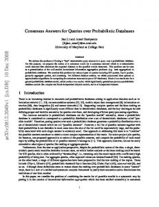
Figure 1: A probabilistic database P DB = ({I1 , I2 , I3 , . . .}, P) with schema R(A, B, C, D); we show only three possible worlds. A a1

B b1

a2

b1

a2

b2

C c1 c2 c3 c1 c2 c4 c5

D d1 d2 d1 d3 d1 d2 d2

P p1 p2 p3 p4 p5 p6 p7

= 0.25 = 0.75 = 0.3 = 0.3 = 0.2 = 0.8 = 0.2

Figure 2: Representation of a disjoint-independent probabilistic database. There are seven possible tuples, which are here grouped by their keys, for readability. There are 16 possible worlds; three are shown in Fig. 1. S k = |Attr(Ri )| is the arity of Ri . Also, denote T up = i T upi the disjoint union of all typed tuples. A database instance is any subset I ⊆ T up that satisfies all key constraints. We write Key(t) for a typed tuple of arity |Key(Ri )| consisting of the key attributes of a tuple t ∈ T upi . The main idea in a probabilistic database is that the state of the database, i.e. the instance I is not known. Instead the database can be in any one of a finite number of possible states I1 , I2 , . . ., called possible worlds, each with some probability. Definition 2.1 A probabilistic database is a probability space P DB = (W, P) where the set of outcomes is a set of possible P worlds W = {I1 , . . . , In }. In other words, it is a function P : W → [0, 1] s.t. I∈W P(I) = 1. Fig. 1 illustrates three possible worlds of a probabilistic database. There are more than three worlds in this probabilistic database, and their probabilities must sum up to 1. The intuition is that we have a database with schema R(A, B, C, D) (underlined attributes are key attributes), but we are not sure about the content of the database: there are several possible contents, each with a probability. 3

A Boolean query q (i.e. a closed First Order Logic sentence) defines the event {IP | I |= q} over a probabilistic database, and its marginal probability is P(q) = I∈W :I|=q P(I). To any tuple t we associate the Boolean query t ∈ I P and denote its marginal probability P(t) = I∈W :t∈I P(I). Note that t 6= t0 and Key(t) = Key(t0 ) implies P(t, t0 ) = 0, i.e. t, t0 are disjoint events. Disjoint-Independent Databases In practice we cannot enumerate all possible worlds, since there are usually too many. Instead, we need to find some concise way to represent the probabilistic database. The representation problem for probabilistic database is an active research topic [17, 7, 27, 5, 4, 27]. In our discussion we restrict to a simple, yet popular representation formalism that can represent all disjoint-independent databases. Any tuple that occurs in some possible world is called a possible tuple for the probabilistic database, and we denote T the set of possible tuples. The representation formalism is simply this: for each relation name Ri we store the set of all possible tuples of type Ri together with their marginal probabilities. If the probabilistic database is disjoint-independent, then one can recover the entire probability space from these marginal tuple probabilities. More precisely, call a probabilistic database disjoint-independent if any set of possible tuples with distinct keys is independent: ∀t1 , . . . , tn ∈ T , Key(ti ) 6= Key(tj ) for i 6= j implies P(t1 , . . . , tn ) = P(t1 ) · · · P(tn ). It suffices to consider only sets of tuples with distinct keys because if any two tuples have the same key then they are disjoint events, and then P(t1 , . . . , tn ) = 0. Thus, in a disjoint-independent database all tuples are independent, except for the tuples that have conflicting keys (which are disjoint). If, in addition, for every relation Ri in the schema, Key(Ri ) = Attr(Ri ), then there are no disjoint tuples, and we say that the probabilistic database is independent. Let K = {Key(t) | t ∈ T } and let I ⊆ T be an instance. For every key there exists a (necessarily unique) tuple t ∈ I value k ∈ K denote pIk = P(t) if P s.t. Key(t) = k, and pIk = 1 − t∈T :Key(t)=k P(t) if there is no tuple t ∈ I Q s.t. Key(t) = k. Then one can check that P(I) = k∈K pIk . In other words, for a disjoint-independent database the probability distribution P(−) can be recovered completely from the marginal probabilities P(t) for all possible tuples t ∈ T.

3

Query Evaluation

We study the query evaluation problem: given a query q and a disjoint-independent database P DB, compute the probability P(q). We first describe the connection between this problem and the probability of Boolean formulas, which has been studied in the literature; in particular it follows that for any fixed q (i.e. any First Order sentence), computing P(q) is in #P in the size of P DB. We then analyze the data complexity of P(q) for a fixed query, and establish a dichotomy for conjunctive queries without self-joins: every query is either #P-hard or in PTIME. A conjunctive query is an FO sentence consisting of positive literals, ∧ and ∃, while a conjunctive query without selfjoins is one in which each relation 4

symbol occurs at most once.

From Queries to Boolean Formulas ¯ = {X1 , . . . , Xn }. A disjoint-independent probConsider n Boolean variables X ¯ ability space with outcomes 2X (the set of truth assignments) is given by a ¯ = X ¯ ¯ ¯ partition X P 1 ∪ . . . ∪ Xm and a probability function P : X → [0, 1] s.t. ∀j = 1, m, ¯ j P(X) ≤ 1. A truth assignment is chosen at random by X∈X ¯ j at most one variable Xi that will be set independently choosing in each set X to true, while all others are set to false: namely Xi is chosen with probability P(Xi ). We will assume that all probabilities are given as rational numbers, P(Xi ) = pi /qi , i = 1, n, where pi , qi are integers. ¯ j | = 1 (i.e. there are no We call this probability space independent if ∀j, |X disjoint variables), and uniform if it is independent and ∀i, P(Xi ) = 1/2. Let Φ be a Boolean P formula over X1 , . . . , Xn ; the goal is to compute its probability, P(Φ) = θ∈2X¯ :θ(Φ) P(θ). The complexity class #P consists of problems of the following form: given an NP machine, compute the number of accepting computations [38]. Let #Φ denote the number of satisfying assignments for Φ. Valiant [47] has shown that the problem: given Φ, compute #Φ, is #P-complete. A statement like “computing P(Φ) is in #P” is technically non-sense, because computing P(Φ) is not a counting problem. However, one can show that ¯ into m sets X ¯1, . . . , X ¯ m , there exists a polynomial-time for any partition of X computable, numerical function F (p1 , q1 , . . . , pn , qn ) s.t. for every formula Φ, the number F · P(Φ) is an integer, and computing F · P(Φ) is in #P. For example, in the case of a uniform distribution, the function F is F = 2n , because in this case 2n · P(Φ) = #Φ, and computing #Φ is in #P. In this sense: Theorem 3.1 [25, 16] Computing P(Φ) is in #P. While computing P(Φ) for a DNF Φ is still #P-hard, Luby and Karp [34] have shown that it has a FPTRAS (fully poly-time randomized approximation scheme). More precisely: there exists a randomized algorithm A with inputs Φ, ε, δ, which runs in polynomial time in |Φ|, 1/ε, and 1/δ, and returns a p/p − 1| > ε) < δ. Here PA denotes the probability over the value p˜ s.t. PA (|˜ random choices of the algorithm. Gr¨adel et al. [25] show how to extend this to independent probabilities, and we have extended it to disjoint-independent probabilities [16]: Theorem 3.2 Computing P(Φ) for a disjoint-independent probability space P and a DNF formula Φ has a FPTRAS. We now establish the connection between the probability of Boolean expressions and the probability of a query on a disjoint-independent database. Let P DB = (T, P) be a database with possible tuples T = {t1 , . . . , tn }. Associate a Boolean variable Xi to each tuple ti and define a disjoint-independent probability space on their truth assignments by partitioning the variables Xi according 5

to their keys (Xi , Xj are in the same partition iff Key(ti ) = Key(tj )), and by defining P(Xi ) = P(ti ). This creates a one-to-one correspondence between the ¯ possible worlds of P DB and the truth assignments 2X , which preserves the probabilities. Consider a Boolean query, q, expressed in First Order Logic (FO) over the vocabulary R. The intensional formula associated to q and database P DB is DB a Boolean formula ΦP , or simply Φq when P DB is understood from the q context, defined inductively as follows: 

Xi f alse

if R(¯ a) = ti ∈ T if R(¯ a) 6∈ T

ΦR(¯a)

=

Φtrue

= true Φf alse = f alse Φ¬q = ¬(Φq )

Φq1 ∧q2

=

Φ∃x.q(x)

=

Φq1 ∧ Φq2 Φq1 ∨q2 = Φq1 ∨ Φq2 _ ^ Φq[a/x] Φ∀x.q(x) = Φq[a/x] a∈D

a∈D

Here D represents the active domain of P DB (i.e. all constants occurring in any possible tuple in T ), q[a/x] denotes the formula q where the variable x is substituted with a, and interpreted predicates over constants (e.g. a < b or a = b) are replaced by true or f alse respectively. If q has v variables, then the size of Φq is O(|q| · |D|v ). The connection between Boolean formulas and Boolean queries is: Proposition 3.3 For every query q and any database P DB = (T, P), P(q) = P(Φq ). A Boolean conjunctive query is a formula of the form q = ∃¯ x.g1 ∧ . . . ∧ gk , where each gi is a positive atomic literal Rj (. . .), called a subgoal. We write q as: q

= g1 , g2 , . . . , gk

(1)

Obviously, in this case Φq is a positive DNF expression. For a simple illustration, suppose q = R(x), S(x, y) and that we have five possible tuples: t1 = R(a), t2 = R(b), t3 = S(a, c), t4 = S(a, d), t5 = S(b, d) to which we associate the Boolean variables X1 , X2 , Y1 , Y2 , Y3 , then Φq = X1 Y1 ∨ X1 Y2 ∨ X2 Y3 . Our discussion implies: Theorem 3.4 For a fixed a Boolean query q, computing P(q) on a disjointindependent database (1) is in #P, (2) admits a FPTRAS when q if conjunctive [25].

A Dichotomy for Queries without Self-joins We now establish the following dichotomy for queries without self-joins: computing P(q) is either #P-hard or is in PTIME in the size of the database 6

P DB = (T, P). A query conjunctive q is said to be without self-joins if each relational symbol occurs at most once in the query body [15, 14]. For example R(x, y), R(y, z) has self-joins, R(x, y), S(y, z) does not. Theorem 3.5 For each of the queries below (where k, m ≥ 1), computing P(q) is #P-hard in the size of the database: h1

= R(x), S(x, y), T (y)

h+ 2 h+ 3

= R1 (x, y), . . . , Rk (x, y), S(y) = R1 (x, y), . . . , Rk (x, y), S1 (x, y), . . . , Sm (x, y)

The underlined positions represent the key attributes, thus, in h1 the database + is tuple independent, while in h+ 2 , h3 it is disjoint-independent. When k = m = 1 then we omit the + superscript and write: h2

= R(x, y), S(y)

h3

= R(x, y), S(x, y)

The significance of these three (classes of) queries is that the hardness of any other conjunctive query without self-joins follows from a simple reduction from one of these three (Lemma 3.7). By contrast, the hardness of these three queries is shown directly [16] (by reducing Positive Partitioned 2DNF [40] to + h1 , and PERMANENT [47] to h+ 2 , h3 ) and these proofs are more involved. Previously, the complexity has been studied only for independent probabilistic databases. De Rougemont [18] claimed that it is is in PTIME. Gr¨adel at al. [18, 25] corrected this and proved that the query R(x), R(y), S1 (x, z), S2 (y, z) is #P-hard, by reduction from regular (non-partitioned) 2DNF: note that this query has a self-join (R occurs twice); h1 does not have a self-join, and was + first shown to be #P-hard in [15]. The hardness of h+ 2 and h3 was discussed in [14, 16]. A PTIME Algorithm We describe here an algorithm that evaluates P(q) in polynomial time in the size of the database, which works for some queries, and fails for others. We need some notations. V ars(q) and Sg(q) are the set of variables, and the set of subgoals respectively. If g ∈ Sg(q) then V ars(g) and KV ars(g) denote all variables in g, and all variables in the key positions in g: e.g. for g = R(x, a, y, x, z), V ars(g) = {x, y, z}, KV ars(g) = {x, y}. For x ∈ V ars(q), let sg(x) = {g | g ∈ Sg(q), x ∈ KV ars(g)}. Given a database P DB = (T, P), D is its active domain (i.e. the set of all constants that occur in any of the tuples in T ). Algorithm 3.1 computes P(q) by recursion on the structure of q. If q consists of two connected components q1 , q2 , then it returns P(q1 )P(q2 ), e.g. P(R(x), S(y, z), T (y)) = P(R(x))P(S(y, z), T (y)). If some variable x occurs in a key position in all Q subgoals, then it applies the independent-project rule: e.g. P(R(x)) = 1 − a∈D (1 − P(R(a))) (this is the probability that R is nonempty). For another example, we apply an independent project on x in 7

Algorithm 3.1 Safe-Eval Input: query q and database P DB = (T, P) Output: P(q) 1: Base Case: if q = R(¯ a) return if R(¯ a) ∈ T then P(R(¯ a)) else 0 2: Join: if q = q1 , q2 and V ars(q1 ) ∩ V ars(q2 ) = ∅ return P(q1 )P(q2 ) 3: Independent project: if sg(x) = Sg(q) Q return 1 − a∈D (1 − P(q[a/x])) 4: Disjoint project: if ∃g(x ∈ V ars(g), KV ars(g) = ∅) P return a∈D P(q[a/x]) 5: Otherwise: FAIL

q = R(x, y), S(x, y): this is correct because q[a/x] and q[b/x] are independent events whenever a 6= b. If there exists a subgoal g whose key positions are constants, then it applies a disjoint project on any variable in g: e.g. x is such a variable in q = R(x, y), S(c, d, x), and any two events q[a/x], q[b/x] are disjoint because of the S subgoal. We call a query safe if algorithm Safe-Eval terminates successfully; otherwise we call it unsafe. Safety is a property that depends only on the query q, not on the database P DB, and it can be checked in PTIME in the size of q by simply running the algorithm over a domain of size 1, D = {a}. Proposition 3.6 [16] For any safe query q, the algorithm computes correctly P(q) and runs in time O(|q| · |D||V ars(q)| ). We first described Safe-Eval in [14], in a format more suitable for an implementation, by translating q into an algebra plan using joins, independent projects, and disjoint projects. Andritsos et al. [3] describe a query evaluation algorithm similar in spirit but for a more restricted class of queries. The Dichotomy Property We define below a rewrite rule q ⇒ q 0 between two queries, where g, g 0 denote subgoals. The intuition is that if q ⇒ q 0 then evaluating P(q 0 ) can be reduced in polynomial time to evaluating P(q). (R1) q (R2) q (R3) q (R4) q, g (R5) q, g

⇒ ⇒ ⇒ ⇒ ⇒

q[a/x] q1 q[y/x] q q, g 0

if x ∈ V ars(q), a ∈ D if q = q1 , q2 , V ars(q1 ) ∩ V ars(q2 ) = ∅ if ∃g ∈ Sg(q), x, y ∈ V ars(g) if KV ars(g) = V ars(g) if KV ars(g 0 ) = KV ars(g), V ars(g 0 ) = V ars(g), arity(g 0 ) < arity(g)

The rules are designed such that whenever q ⇒ q 0 then the evaluation of q 0 on a disjoint-independent database P DB 0 can be easily reduced to the evaluation of q on some other disjoint-independent database P DB. For example, rule (R4) allows us to drop a subgoal g: to evaluate q 0 on P DB 0 simply add a relation for 8

g and make it deterministic by setting all tuple probabilities P(t) = 1. This is possible because KV ar(g) = V ar(g), i.e. all variables occur some key position, like in R(x, y, z, x, a): for every key value we need only one possible tuple with that key value, hence we can set its probability = 1. Similarly, rule (R5) allows us to replace a subgoal g with another subgoal g 0 by dropping some variables and/or constants, provided that g 0 has the same set of variables in key positions, and the same set of variables (in key and non-key positions). Lemma 3.7 If q ⇒∗ q 0 and q 0 is #P-hard, then q is #P-hard. Thus, ⇒ gives us a convenient tool for checking if a query is hard, by trying to rewrite it to one of the known hard queries. For example, consider the queries q and q 0 below: Safe-Eval fails immediately on both queries, i.e. none of its cases apply. We show that both are hard by rewriting them to h1 and h+ 3 respectively. By abuse of notations we reuse the same relation name for g and g 0 when applying rule (R5) (e.g. S in the second line and S in the third line should strictly speaking be different relation symbols): q (R4) (R5) q0 (R3) (R4)

= ⇒ ⇒∗ = ⇒ ⇒

R(x), R0 (x), S(x, y, y), T (y, z, b) R(x), S(x, y, y), T (y, z, b) R(x), S(x, y), T (y) = h1 R(x, y), S(y, z), T (z, x), U (y, x) R(x, y), S(y, x), T (x, x), U (y, x) R(x, y), S(y, x), U (y, x) = h+ 3

Call a query q final if it is unsafe, and ∀q 0 , if q ⇒ q 0 then q 0 is safe. Clearly every unsafe query rewrites to a final query: simply apply ⇒ repeatedly until all rewritings are to safe queries. One can prove: + Lemma 3.8 h1 , h+ 2 , h3 are the only final queries.

This implies immediately the dichotomy property: Theorem 3.9 Let q be a query without self-joins. Then one of the following holds: + • q is unsafe and q rewrites to one of h1 , h+ 2 , h3 . In particular, q is #P-hard.

• q is safe. In particular, it is in PTIME. + Proof: We need to show that q is unsafe iff it rewrites to one of h1 , h+ 2 , or h3 . The important direction results from Lemma 3.8 and our discussion above: if q is unsafe, then it rewrites to one of these three queries. For other direction we need to show that if q is safe, then q does not rewrite to any of the queries h1 , h+ 2 , or h+ . Note that this follows trivially if one assumes PTIME = 6 #P. A direct proof 3 proceeds by induction on the number of recursion steps taken by Algorithm Safe-Eval on the query q. The Base Case in the algorithm (q = R(¯ a)) is obvious: q does not rewrite to anything. For the Join case, q = q1 , q2 , we

9

note that if q rewrites to one of the three h-queries then so must either q1 or q2 . For the Independent project case, there is some variable x occurring in key positions in all subgoals of q. If q ⇒∗ hi , for some i = 1, 2, 3 then that variable must be removed somehow, and the only rule that can eliminate it is (R1), which substitutes x with a constant. But then one can prove that q[a/x] ⇒∗ hi , contradicting the induction hypothesis. For the Disjoint Project case, we note that the subgoal g has no variables in key positions, hence it must be eliminated by rule (R2) (If rule (R4) ever applies to g, then Rule (R2) also applies, since KV ar(g) = ∅ implies V ar(g) = ∅, hence g is disconnected from the rest of the query.) In other words, x belongs to a connected component that is eliminated during the rewriting q ⇒∗ hi , hence we also have q[a/x] ⇒∗ hi , contradiction. 2 The Complexity of the Complexity We complete our analysis by studying the following problem: given a relational schema R and conjunctive query q without self-joins over R, decide whether q is safe1 . We have seen that this problem is in PTIME; here we establish tighter bounds: Proposition 3.10 [16] (1) The problem: “given an independent schema R (i.e. Key(Ri ) = Attr(Ri ) for all Ri ∈ R) and a query q, decide whether q is safe” is in AC 0 . (2) The problem: “given a disjoint-independent schema R (i.e. Key(Ri ) ⊆ Attr(Ri ) for all Ri ∈ R) and a query q, decide whether q is safe” is PTIME complete.

4

Conclusions and Future Challenges

In many applications today it is becoming prohibitively expensive, and even impossible, to enforce a precise semantics, by completely cleaning the data and removing all types of uncertainties. Probabilistic databases manage data with an explicit representation and quantification of uncertainties, and query evaluation becomes a special form of probabilistic inference. Probabilistic databases need to scale both in the size of the data, and in the complexity of the probabilistic model. Scaling in any of these two dimensions is a challenging problem. Consider the size of the data. Most often the data does not fit in main memory, but instead needs to be read from disk, sequentially or using some index. One approach to scale query processing is to restrict the query evaluation on only the top k answers: that is, the answers to a (nonBoolean) query are ranked in decreasing order of their probability score, and only the top k are returned to the user, where k is a small number, typically 10 or 20. While there may be many (e.g. thousands) of possible answers, the systems computes only the top k, and thus needs to do far fewer probabilistic inferences. But this creates a chicken and egg problem: we do not know which tuples are the top k until we have evaluated all probabilities [41]. In addition, probabilistic databases need to handle more complex probabilistic models than the disjoint-independent databases discussed in this paper. 1 For a fixed R there are only finitely many queries without self-joins: this is the reason why R is part of the input.

10

Correlations between tuples or attribute values occur naturally in practice: for example in information extraction, the extraction of one data item may depend on the extraction of a previous item, hence the two items are correlated probabilistic events [28]. The explicit representation of such correlations in probabilistic databases is called lineage, or provenance [7, 26], and it complicates significantly the query evaluation problem. Some simple database optimization techniques, such as predicate pushdown or semijoin reduction, still help, but they are limited in scope. More powerful optimization techniques currently used in database systems, such as using materialized views during query processing, become difficult to use because of the extra cost of the lineage information. A new line of research seeks to simplify the lineage information by either finding an equivalent but simpler lineage [42], or by using Fourier approximations of Boolean expressions to approximate the lineage [43]. Acknowledgments The author was partially supported by NSF Grants IIS-0713576, IIS-0513877, IIS-0627585 IIS-0428168, IIS-0454425 and a Gift from Microsoft.

References [1] S. Abiteboul and P. Senellart. Querying and updating probabilistic information in XML. In EDBT, pages 1059–1068, 2006. [2] E. Adams. A Primer of Probability Logic. CSLI Publications, Stanford, California, 1998. [3] P. Andritsos, A. Fuxman, and R. J. Miller. Clean answers over dirty databases. In ICDE, 2006. [4] L. Antova, C. Koch, and D. Olteanu. 10^(10^6) worlds and beyond: Efficient representation and processing of incomplete information. In ICDE, 2007. [5] L. Antova, C. Koch, and D. Olteanu. World-set decompositions: Expressiveness and efficient algorithms. In ICDT, pages 194–208, 2007. [6] F. Bacchus, A. Grove, J. Halpern, and D. Koller. From statistical knowledge bases to degrees of belief. Artificial Intelligence, 87(1-2):75–143, 1996. [7] O. Benjelloun, A. Das Sarma, A. Halevy, and J. Widom. ULDBs: Databases with uncertainty and lineage. In VLDB, pages 953–964, 2006. [8] G. Borriello and F. Zhao. World-Wide Sensor Web: 2006 UW-MSR Summer Institute Semiahmoo Resort, Blaine, WA, 2006. www.cs.washington.edu/mssi/2006/schedule.html. [9] T. Choudhury, M. Philipose, D. Wyatt, and J. Lester. Towards activity databases: Using sensors and statistical models to summarize people’s lives. IEEE Data Eng. Bull, 29(1):49–58, March 2006. 11

[10] E. F. Codd. A relational model for large shared databank. Communications of the ACM, 13(6):377–387, June 1970. [11] G. Cooper. Computational complexity of probabilistic inference using bayesian belief networks (research note). Artificial Intelligence, 42:393– 405, 1990. [12] R. Cowell, P. Dawid, S. Lauritzen, and D. Spiegelhalter, editors. Probabilistic Networks and Expert Systems. Springer, 1999. [13] P. Dagum and M. Luby. Approximating probabilistic inference in bayesian belief networks is NP-hard. Artificial Intelligence, 60:141–153, 1993. [14] N. Dalvi, C. Re, and D. Suciu. Query evaluation on probabilistic databases. IEEE Data Engineering Bulletin, 29(1):25–31, 2006. [15] N. Dalvi and D. Suciu. Efficient query evaluation on probabilistic databases. In VLDB, Toronto, Canada, 2004. [16] N. Dalvi and D. Suciu. Management of probabilistic data: Foundations and challenges. In PODS, pages 1–12, Beijing, China, 2007. (invited talk). [17] A. Das Sarma, O. Benjelloun, A. Halevy, and J. Widom. Working models for uncertain data. In ICDE, 2006. [18] M. de Rougemont. The reliability of queries. In PODS, pages 286–291, 1995. [19] A. Deshpande, C. Guestrin, S. Madden, J. M. Hellerstein, and W. Hong. Model-driven data acquisition in sensor networks. In VLDB, pages 588–599, 2004. [20] A. Deshpande, C. Guestrin, S. Madden, J. M. Hellerstein, and W. Hong. Using probabilistic models for data management in acquisitional environments. In CIDR, pages 317–328, 2005. [21] O. Deux. The story of O2 . IEEE Transactions on Knowledge and Data Engineering, 2(1):91–108, March 1990. [22] A. Doan, R. Ramakrishnan, F. Chen, P. DeRose, Y. Lee, R. McCann, M. Sayyadian, and W. Shen. Community information management. IEEE Data Engineering Bulletin, Special Issue on Probabilistic Data Management, 29(1):64–72, March 2006. [23] M. B. et al. Data management in the world-wide sensor web. IEEE Pervasive Computing, 2007. To appear. [24] O. Etzioni, M. Cafarella, D. Downey, S. Kok, A. Popescu, T. Shaked, S. Soderland, D. Weld, and A. Yates. Web-scale information extraction in KnowItAll: (preliminary results). In WWW, pages 100–110, 2004.

12

[25] E. Gr¨ adel, Y. Gurevich, and C. Hirsch. The complexity of query reliability. In PODS, pages 227–234, 1998. [26] T. Green, G. Karvounarakis, and V. Tannen. Provenance semirings. In PODS, pages 31–40, 2007. [27] T. Green and V. Tannen. Models for incomplete and probabilistic information. IEEE Data Engineering Bulletin, 29(1):17–24, March 2006. [28] R. Gupta and S. Sarawagi. Creating probabilistic databases from information extraction models. In VLDB, pages 965–976, 2006. [29] A. Halevy, A. Rajaraman, and J. Ordille. Data integration: The teenage years. In VLDB, pages 9–16, 2006. [30] D. Heckerman. Tutorial on graphical models, June 2002. [31] E. Hung, L. Getoor, and V. Subrahmanian. PXML: A probabilistic semistructured data model and algebra. In ICDE, 2003. [32] T. Imielinski and W. Lipski. Incomplete information in relational databases. Journal of the ACM, 31:761–791, October 1984. [33] T. Jayram, R. Krishnamurthy, S. Raghavan, S. Vaithyanathan, and H. Zhu. Avatar information extraction system. IEEE Data Engineering Bulletin, 29(1):40–48, 2006. [34] R. Karp and M. Luby. Monte-Carlo algorithms for enumeration and reliability problems. In Proceedings of the annual ACM symposium on Theory of computing, 1983. [35] N. Khoussainova, M. Balazinska, and D. Suciu. Towards correcting input data errors probabilistically using integrity constraints. In MobiDB, pages 43–50, 2006. [36] G. Kuper, L. Libkin, and J. P. (Eds.). Constraint Databases. Springer, 2000. [37] J. Lester, T. Choudhury, N. Kern, G. Borriello, and B. Hannaford. A hybrid discriminative/generative approach for modeling human activities. In IJCAI, pages 766–772, 2005. [38] C. Papadimitriou. Computational Complexity. Addison Wesley Publishing Company, 1994. [39] S. Philippi and J. Kohler. Addressing the problems with life-science databases for traditional uses and systems biology. Nature Reviews Genetics, 7:481–488, June 2006. [40] J. S. Provan and M. O. Ball. The complexity of counting cuts and of computing the probability that a graph is connected. SIAM J. Comput., 12(4):777–788, 1983. 13

[41] C. Re, N. Dalvi, and D. Suciu. Efficient Top-k query evaluation on probabilistic data. In ICDE, 2007. [42] C. Re and D.Suciu. Materialized views in probabilistic databases for information exchange and query optimization. In Proceedings of VLDB, 2007. [43] C. Re and D. Suciu. Approximate lineage for probabilistic databases. Technical Report 2008-03-02, University of Washington, Seattle, WA, 2008. [44] H.-J. Schek and M. H. Scholl. The relational model with relation-valued attributes. Information Systems, 11(2):137–147, 1986. [45] R. Snodgrass. The temporal query language TQUEL. ACM Transactions on Database Systems, 12(2):247–298, June 1987. [46] D. Suciu. An overview of semistructured data. SIGACT News, 29(4):28–38, December 1998. [47] L. Valiant. The complexity of enumeration and reliability problems. SIAM J. Comput., 8:410–421, 1979. [48] M. van Keulen, A. de Keijzer, and W. Alink. A probabilistic XML approach to data integration. In ICDE, pages 459–470, 2005. [49] M. Y. Vardi. The complexity of relational query languages. In Proceedings of 14th ACM SIGACT Symposium on the Theory of Computing, pages 137–146, San Francisco, California, 1982.

14