DDL.1: A Formal Description of a Constraint Representation Language for Physical Domains Amedeo Cesta IP-CNR National Research Council of Italy Viale Marx 15, I-00137 Rome, Italy
[email protected]
Angelo Oddi Dipartimento di Informatica e Sistemistica Universit`a di Roma “La Sapienza” Via Salaria 113, I-00198 Rome, Italy
[email protected]
Abstract. This paper describes a domain description language DDL.1 able to represent physical domains to solve planning and scheduling problems. DDL.1 uses a representation, inspired by classical control theory, based on state-variables to represent the relevant features of a domain. Each state variable is meant to represent a set of plausible temporal evolutions those features may have. DDL.1 allows to specify constraints on the sequence of values that a state variable may assume over time. For the language a syntactic specification, and a model theoretic semantic are given. The problem of temporal planning using a DDL.1 specification is also addressed and a planning algorithm named TP-SV introduced. The paper tries to show how this kind of description languages may generate a methodology to gracefully model the relevant constraints in physical domains, and how a formally specified planner may be associated to this description.
1
Introduction
In current planning research quite a lot of formal work has been produced to understand and precisely characterize the power of classical planning frameworks ([3, 13, 2, 8] and many others). This work has allowed the specification of a clear semantics for the proposed formalisms and the investigation of the computational complexity of several reasoning processes. Still a gap exists between those works and application-oriented proposals. The difference lies in the problems and domains considered: quite simplified in the former case, more sophisticated in the latter. Unfortunately application-oriented work usually lacks a sufficient theoretical analysis. Of course, from both sides attempts can be mentioned to fill this gap, examples may be on one side Tate’s formalism [17], and on the other the Zeno planner [14]. This middle-ground work has the aim of dealing with more complex domains while following a principled approach that allows the generalization of results. Following this trend, this paper re-considers a particular proposal, the HSTS architecture [10, 11], and develops a formal analysis of the representation language proposed in it. This work is somewhat preliminary, it makes a first step towards the investigation of the computational properties of the framework and should be continued both studying the computational complexity of specialized reasoning and deeply investigating those aspects of the language that may be useful to speed up planning. The domain description is a fundamental initial step to address both planning and scheduling problems. Knowledge-based domain independent planners are endowed with
In M.Ghallab, A.Milani (Eds), New Directions in AI Planning, IOS Press, 1996 a Domain Description Language (DDL). A DDL is a Knowledge Representation Language that allows users to specify the basic components of a domain, to associate a description to those components, and to specify the constraints and mutual relationships among components. Classical planners usually refer to the description language derived from STRIPS [3, 13]. Application oriented planners are endowed with their own peculiar DDLs, for example the Task Formalism in O-Plan [4], and the specialized languages used in OPIS [16], and HSTS [10, 11]. In our view, some aspects first proposed in the HSTS domain description language are of interest to the current debate because: (a) the language is aimed at describing complex domains in which planning and scheduling aspects are intermixed; (b) the representation suggests a methodology for guiding a user to describe a domain (a usually neglected aspect in planning research); (c) domains are described in terms of the constraints involved, thus naturally enabling the construction of constraint posting planners. What we propose in this paper is a formal account of a representation language named DDL.1, that uses the same ontology of the HSTS-DDL, but is restricted in its expressive power in order to develop a clear semantics and to specify a temporal planner that exploits the formalized aspects of the language. Although the used ontology exploits ideas from control theory [7] we propose here a formal account that refers to classical AI studies for describing both the semantics of the language and the planning process. The paper is organized as follows: Section 2 introduces the features of DDL.1 language. Section 3 describes more specifically the way of describing constraints in DDL.1 and presents the language complete syntax, while Section 4 presents its semantics. Sections 5 proposes a temporal planner that actually uses the formalism. Section 6 shortly discusses related research while Section 7 concludes the paper.
2
DDL.1 General Features
DDL.1 representation adopts basic ideas from control theory [7, 5] extended to allow the specification of constraints. The planning problem is seen as the problem of deciding the behavior of a dynamic domain. The behavior of a domain (its temporal evolution) is seen as the continuous interaction among different components. Each domain component is represented using state variables; a single state variable (SV) is a relevant feature of the component. DDL.1 allows the intensional description of any plausible temporal evolution of the state variables. Such evolution is defined describing the set of values a SV may assume over time, and a set of constraints, named compatibilities, a value should satisfy when assumed by the related SV. In DDL.1 state variables’ values are restricted to a discrete set and are instances of predicates of the form P (x1 , . . . , xm ). More formally, for each state variable SVi , DDL.1 allows the specification of: • a set DPSVi of the value-predicates P (x1 ,. . . , xm ); • the domain DVj of each variable xj appearing in the value-predicates; From these two sets the set DSVi of the state-variable values can be defined. DSVi is the set of the ground terms obtained by substituting the variables in DPSVi with the domain values DVj . The dynamics of a state variable SVi is defined as the set Σi of all the functions si : T → DSVi where T is the discrete set of time instants. Given the definition of each SV, the set ∆ of the domain evolutions may be defined as: ∆ = Σ1 ×Σ2 ×. . .×Σn .
In M.Ghallab, A.Milani (Eds), New Directions in AI Planning, IOS Press, 1996 By defining compatibilities DDL.1 allows the user to represent constraints on the legal sequences of values that a state variable may assume over time. A given value may be constrained by different values on the same state variable, and by values on different state variables. Those further constraints express the domain theory, namely the description of the domain laws in terms of reciprocal adaptability, synchronization, and dependency relations among values. By constraining the situations in which a given value may be taken by a state variable a generic compatibility C represents a restriction of the possible evolutions of the domain, that is C ⊆ ∆. A (set of) goal(s) in this framework is the specification of a (set of) “desired” value(s) to be taken by SVs. Planning means determining a particular temporal evolution (i.e., a function si : T → DSVi for each state variable SVi ) that satisfies both the goal(s) and all the specified compatibility constraints.
2.1
Representing a Simple Domain
A simple example from a process planning domain may help to show the DDL.1 use. The domain consists of a drilling machine able to create holes of two different diameters by automatically switching between two different bits. The holes are executed when a piece of a certain material is blocked on the support of the drill. A domain model may contain two state-variables named: SVDRILL , that represents the operating status of the drilling tool, and SVSU P P , that represents the operating status of the support. The state-variables’ dynamics is described defining the set of values each SV may assume. In this case: • DPDRILL ={W AIT , BIT1 (x), BIT2 (x)}. W AIT represents an idle state, BIT1 (x) and BIT2 (x) represent a status in which the machine is drilling a hole on the piece x using different bits. • DPSU P P = {BLOCKED(x), F REE}. BLOCKED(x) represents the fact that piece x is ready to be drilled on the support. It should be clear that the values cannot be assumed by state-variables in arbitrary order. For example, a hole can be done only while a piece is blocked on the support. Those constraints are represented using the compatibility specification described in detail in the next Section.
3
Describing Constraints on Domain Temporal Evolutions
To sum up, a domain description that can be built by a DDL.1 specification contains state-variables, state-variable values, and compatibilities. Compatibilities allow the user to represent constraints on the legal sequences of values that a state variable may assume. A given value may be constrained either by different values on the same state variable, and/or by values on different state variables. A compatibility asserts an intensional constraint on the behavior of a state variable. Such constraint consists of two components: (a) a causal component that defines a causal relation between two values: a reference value and a constraining value; (b) a temporal component that specifies a temporal constraint on the causal component. The temporal relation may contain both a qualitative and a quantitative constraint. Table 1 shows the whole specification of the language. May be observed that the causal component of a compatibility are described
In M.Ghallab, A.Milani (Eds), New Directions in AI Planning, IOS Press, 1996 < DomainDef inition > ::= (DOMAIN < DomainN ame > {< StateV ariable >}) < DomainN ame > ::= a constant symbol < StateV ariable > ::= (SV < StateV ariableN ame > < DomainV alues > {< Compatibility >}) < StateV ariableN ame >::= a constant symbol < DomainV alues > ::= < StateV arV alN ame >, {< StateV arV alN ame >} < StateV arV alN ame > ::= a constant symbol < Compatibility > ::= (OR-COMP {< AndComp >}) | < AndComp > < AndComp > ::= (COMP < Ref V alue > (MEETS < ConstrV alue >) (MET-BY < ConstrV alue >) {(DURING < ConstrV alue > < DurationInt >< DurationInt > ) }) < Ref V alue > ::= < V alue > < ConstrV alue > ::= < V alue > < V alue > ::= (< StateV ariableN ame > (< StateV arV alN ame > < V arList >) < DurationInt >) < V arList > ::= { (< V arN ame >:< V arDomain >) } < V arN ame > ::= a constant symbol < V arDomain > ::= application dependent < DurationInt > ::= (< T emporalExpr >< T emporalExpr >) < T emporalExpr > ::= (< F unctionN ame >< V ariableList >) | < T imeConstant > < V ariableList > ::= {< V arN ame >}+ < T imeConstant > ::= 0|1|2| ... |∞ < F unctionN ame > ::= a constant symbol
Table 1: BNF Specification of DDL.1
by the syntactic categories (the reference value) and (the constraining value). The temporal component is specified by a restricted number of the qualitative temporal relations usually defined in the literature [1] (to simplify matters only the MEETS, MET-BY and DURING are allowed). The MEETS and MET-BY relations constrain two values belonging to the same state variable to appear in strict sequence in any legal behavior of the SV (namely, MEETS (MET-BY) states that the end-time (start-time) of the reference value coincide with the start time (end-time) of the constraining value). The DURING relation constrains two values belonging to different state-variables. It is used to express synchronization constraints between the state variables’ behaviors (more specifically DURING states that the start-time of the constraining value precedes the start-time of the reference, and its end-time follows the end-time of the reference).
3.1
Compatibilities in the Drilling Machine Example
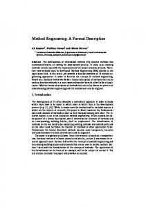
Following the syntax in Table 1 we can describe the domain of the drilling machine according to the model previously introduced. Legal value sequencing are described by using compatibilities. Figure 1 shows the constraints relative to the values of the SVDRILL . It is possible to observe some characteristics of the language: (a) the first compatibility uses an OR-COMP to describe the constraints on the value W AIT . It enumerate the possible legal sequences that include W AIT , one of them should be verified on any legal temporal evolution including W AIT . (b) With MEETS and METBY constraints specification are specified to describe legal value transition on the SV. For example, the second and third compatibilities state the constraint that it is not possible to execute two consecutive holes without intermixing a W AIT value. (c) The DURING temporal relation is used to specify values synchronization between two statevariables. Again, in the second and third compatibilities of Figure 1, a DURING specification states that it is possible to drill with BITi only while a piece is BLOCKED
In M.Ghallab, A.Milani (Eds), New Directions in AI Planning, IOS Press, 1996 (OR-COMP (COMP (DRILL (WAIT) (0 ∞)) (MET-BY (DRILL (BIT1 (x : workpiece)) (d1 (x)D1 (x))))) (MEETS (DRILL (BIT2 (y : workpiece)) (d2 (y)D2 (y))))) (COMP (DRILL (WAIT) (0 ∞)) (MET-BY (DRILL (BIT1 (x : workpiece)) (d1 (x)D1 (x))))) (MEETS (DRILL (BIT1 (y : workpiece)) (d1 (y)D1 (y))))) (COMP (DRILL (WAIT) (0 ∞)) (MET-BY (DRILL (BIT2 (x : workpiece)) (d2 (x)D2 (x))))) (MEETS (DRILL (BIT2 (y : workpiece)) (d2 (y)D2 (y))))) (COMP (DRILL (WAIT) (0 ∞)) (MET-BY (DRILL (BIT2 (x : workpiece)) (d2 (x)D2 (x))))) (MEETS (DRILL (BIT1 (y : workpiece)) (d1 (y)D1 (y))))) (COMP (DRILL (BIT1 (x : workpiece)) (d1 (x)D1 (x))) (MET-BY (DRILL (WAIT) (0 ∞))) (MEETS (DRILL (WAIT) (0 ∞))) (DURING (SUPP (BLOCKED (x : workpiece)) (0 ∞) ) (0 ∞) (0 ∞) )))) (COMP (DRILL (BIT2 (x : workpiece)) (d2 (x)D2 (x))) (MET-BY (DRILL (WAIT) (0 ∞))) (MEETS (DRILL (WAIT) (0 ∞)) ) (DURING (SUPP (BLOCKED (x : workpiece)) (0 ∞) ) (0 ∞) (0 ∞) )))
Figure 1: Compatibility constraints on the state variable DRILL
on the support SVSU P P . Compatibilities related to the SVSU P P are not presented. The only constraint contained in it states that a BLOCKED value should be reasonably followed by a F REE one. For the sake of exemplification of single properties of the language, we have described a very limited behavior of the domain. It should be clear that the same language can be used for more fine-grained descriptions. For example it is possible to explicitly describe and represent the set-up times needed to arrive at different operating status of a certain represented instrument, etc. (see [10, 11] for several examples).
3.2
Some Comments on the Language
The language allows to represent quite complex aspects of the problem domain: (a) temporal evolutions of domain features: in fact, all the value specifications are enriched with duration constraints for the interval of time that a SV assumes the values. Durations are represented by an interval [d, D] where d and D represent minimal and maximal time length; (b) physically realizable transition between values by the MEETS and MET-BY specifications; (c) different processes in the domain behaving in parallel by using state variables; (d) synchronization constraints between parallel processes by using the (DU RIN G inti intf ); (e) simple resource constraints: in fact, we can consider a resource as described by a state-variable, and a value as a reservation on it for a given interval of time. With the syntactic restriction given here we can represent only binary capacity constraints (extensions are investigated in [11]). An interesting aspect to notice is the intuitive and graceful methodology the language makes available to the user for describing the features of the domain. This
In M.Ghallab, A.Milani (Eds), New Directions in AI Planning, IOS Press, 1996 methodology is made possible by having the state variables and their values as first class objects in the language at a symbolic level. Moreover, the compatibility specification allows to describe uniformly an interesting number of constraints governing the domain dynamics. Such constraints are also introduced using the uniform metaphor of the description language. More conventional languages may have a rather similar expressive power but have a representation metaphor different and less user-oriented. In our view, action-centered formalisms in general allow a description of a domain very atomic and disaggregated, not easily controllable by the user.
4
A Model Theoretic Semantics for DDL.1
The constraints stated by compatibility specification bound the number of evolutions of the represented domain (the set ∆ previously introduced). The semantics of any language sentence is defined as the set of the evolutions compatible with the given constraints. To obtain a formal shape for such an intuitive idea some preliminary definitions are needed. Considering the syntax in Table 1, vj denotes an element belonging to the syntactic category of the state variable SVi . We designate with ek a ground element of a temporal evolution of the state variable SVi . It is worth noting that ek is a 3ple: ek =< SVi , p, [ts , te ] >, where p ∈ DSV i and ts ,te ∈ T with ts ≤ te . Given a function si : T → DSV i , an element of evolution ek =< SVi , p, [ts , te ] > is contained in si (t) (denoted by ek v si (t)), if ∃ts and ∃te such that the function si (t) assumes the value p ∈ DSV i in the interval [ts , te ]. An element of evolution ek =< SVi , p, [ts , te ] > is contained in a value vj = < SVi , p(x1 . . . xm ), [d(x1 . . . xm ), D(x1 . . . xm )] > (denoted by ek ⊆ vj ) if a ground instance vjg =< SVi , p, [d, D] > of vj exists such that d ≤ ts −te ≤ D. The DDL.1 semantics is defined by using the function: E : LDDL.1 → 2∆ where LDDL.1 represents the set of sentences allowed by the DDL.1 grammar and 2∆ is the power-set of ∆. As said above, the semantics of a given domain description is a subset of ∆. The subset can be obtained from the intersection of the sets of temporal evolution allowed by each constraint of the language (that is, by each compatibility). A function T given a compatibility c computes the subset of admissible evolutions contained in ∆. The function T is of the kind T : 2∆ × CDDL.1 → 2∆ where CDDL.1 is the set of compatibilities that can be defined using DDL.1. T can be defined as follows (where sSVe represents the temporal evolution s of the SV in which the ground element e is assumed): T (∆, (OR−COM P (AndComp1 ) . . . (AndCompn )) =
Sn
i=1
T (∆, AndCompi )
T (∆, (COM P vref (M EET S vmeets ) (M ET −BY vmet−by ) (DU RIN G vduring1 inti1 intf1 ) . . . (DU RIN G vduringk intik intfk )) = {< sSV 1 (t) . . . sSV n (t) >∈ ∆ | (∃eref ) (∃emeets ) (∃emet−by ) (∃eduring1 ) . . . (∃eduringk ) (eref v sSVeref )∧ (eref ⊆ vref ) ⊃ (emeets v sSVemeets )∧ (emeets ⊆ vmeets ) ∧ PM EET S (eref , emeets )∧ (emet−by v sSVemet−by )∧ (emet−by ⊆ vmet−by ) ∧ PM ET−BY (eref , emet−by )∧ (eduring1 v sSVeduring )∧ (eduring1 ⊆ vduring1 )∧ PDU RIN G (eref , eduring1 , inti1 , intf1 ) 1 ∧...∧ (eduringk v sSVeduring )∧ (eduringk ⊆ vduringk )∧ PDU RIN G (eref , eduringk , intik , intfk )} k
To complete the definition of T , a definition for the temporal predicates PM EET S , PM ET −BY e PDU RIN G is needed. Given any couple of elements e1 = < SV1 , p1 , [ts1 , te1 ] >,
In M.Ghallab, A.Milani (Eds), New Directions in AI Planning, IOS Press, 1996 and e2 =< SV2 , p2 , [ts2 , te2 ] >, and two intervals inti = [di , Di ] and intf = [df , Df ] those predicates are defined as follows: PM EET S (e1 , e2 ) = (ts1 ≤ te1 ) ∧ (ts2 ≤ te2 )∧ (te1 = ts2 ) PM ET −BY (e1 , e2 ) = (ts1 ≤ te1 ) ∧ (ts2 ≤ te2 )∧ (te2 = ts1 ) PDU RIN G (e1 , e2 , inti , intf ) = (ts1 ≤ te1 )∧ (ts2 ≤ te2 )∧ (di ≤ ts1 −ts2 ≤ Di )∧ (df ≤ te2 −te1 ≤ Df )
Finally the formal semantics E can be inductively defined as: 1. E((DOM AIN . . . (SV . . .)T 1 . . . (SV . . .)n )) = n i=1 E((SV . . . (Compatibility1 . . . Compatibilityp ))i ) Tp 2. E((SV . . . (Compatibility1 . . . Compatibilityp ))) = i=1 E(Compatibilityi ) 3. E(Compatibilityi ) = T (∆, Compatibilityi )
It is worth observing that according to this semantics when E((DOM AIN . . .)) = ∅ the domain description is inconsistent.
5
A Temporal Planner with State Variables
The previous Sections introduces a particular language to describe the constraints framing the evolution of a physical domain. This Section deals with the use of the language in a planner. First an intuitive description of what a planner is supposed to do with a DDL.1 specification is given and then a more formal specification of a planning algorithm is presented. To allow comparisons with more conventional planners, we adopt the formal approach currently used in planning literature (e.g., [18]). The language allows the description of a discrete event dynamic system, a dynamic system in which state variables may have temporal evolutions that are piecewise constant functions of time. Such systems are studied in a sub-area of control theory and optimization (see for example [15]). Here we consider as a temporal planning problem the problem of deciding an evolution of such systems. While classical plan-space search planners built a partial plan that necessarily asserts a conjunction of predicates (goals) in any possible completion, here a planner searches in the state variable temporal evolution space to determine those evolutions that necessarily include certain piece of evolution given as goals. In other words, planning is this framework consists of determining the elements of a matrix S × T where S is the space of the state variables and T is the time line. Some of the values (with a temporal duration) are given as goals and the planner should find a ”convenient position” on the matrix for those values and fill the rest of the matrix with values compatible with the goal positioning (i.e., any positioned value should satisfy all the constraints specified in the DDL.1 domain definition). This view of planning was first used in HSTS [10, 11]. The rest of this Section describes a planning algorithm, named TP-SV (Temporal Planner with State Variables) which works in the framework sketched above. A TP-SV goal is a 3-ple g = (vp tr vc ) where vp and vc are values of the kind vj =< SVi , p(x1 . . . xm ), [d(x1 . . . xm ), D(x1 . . . xm )] >. Both vp and vc may be either ground or unground. The tr is either one of the temporal constraints or nil representing a null constraint: tr ∈ {(MEETS), (MET-BY), (DURING inti intf )} ∪ {nil} A user goal may be described as the 3-ple: (nil nil vcg ) where vcg is a completely ground value. The goal definition allows to represent as planner’s goal all the constraints that should be implemented in the solution. Both the external goals defined by the user
In M.Ghallab, A.Milani (Eds), New Directions in AI Planning, IOS Press, 1996 and the domain goal generated by the compatibility specification are represented with a 3-ple. The value vp is intended to be a value existing yet in the current solution which produces (the subscript p stands for producer) a constraint that requires a new value vc (c stands for consumer) according to the temporal relation tr. At present users goals are ground pieces of evolution independent from each other, this is represented by the nil “producer” and the nil “temporal constraint”. A plan in TP-SV is a 4-ple P =< E, O, L, B > where: • E is the set of values assumed by the state variables SVi E = {v11 , . . . , v1n1 , . . . , vj1 , . . . , vjnk } • O is the set of ordering relations among the elements of E. That is O is a set of elements of the kind (< tsp , tep > tr < tsc , tec >). Where tr represents the temporal relation among the values vp e vc , and the couple of temporal variables < tsp , tep > (< tsc , tec >) represents the start-time and end-time of the duration interval associated to vp (vc ). • L = {(vp1 vc1 ), . . . , (vpm vcm )} stores the causal relations among elements of E (the set of causal links). Two elements vp and vc are each other related by a causal link if the insertion of the element vp in the domain directly caused the insertion of the element vc in order to satisfy a compatibility constraint (a goal). • B is the set of bindings performed on the variables associated to DDL.1’s values during the planning process. B is a set of couples (x, y) meaning that variables x is substituted with term y. The planning algorithm TP-SV is shown in Figure 2. The algorithm builts a ground evolution of the domain by incrementally posting goals (constraints) on a partial solution. TP-SV has three input parameters: a plan P , the list of goals to be achieved, and the domain theory Λ of DDL.1 constraints specification. The planner is given a set of user’s goals and starts working on an empty plan P0 in which any state variable SVi is set to a steady rest evolution represented with the 0 00 sequence of values (v0i Ui v0i ). The value v0i is a rest value that should be defined for any state-variable. The value U (undefined) initially represents the stretch of temporal evolution that the planner should define to satisfy goals. A plan is seen as a sequence of value transitions that starts from some rest values, evolves to satisfy some goals and return to the rest values. More formally the empty plan P0 is a 4-ple P0 =< E0 , O0 , L0 , B0 >: 0 00 • E0 = {. . . v0i Ui v0i . . .} • L0 = {} m m 0 0 00 00 • O0 = {. . . < ts0i , te0i >≺< tsUi , teUi >, < tsUi , teUi >≺< ts0i , te0i > . . .} • B0 = {} m
The symbol ≺ stands for MEETS. Some further observation are worth doing to understand the algorithm in Figure 2: (a) the planner uses the non-deterministic operator choose to start separate computations in choice points; (b) to perform Step 3.a of the algorithm the value vp and the tr contained in the goal are used to filter the possible positions to actually implement the constraint; (c) at Step 5 and 6 the MGU operator computes the Most General Unifier among its parameters.
In M.Ghallab, A.Milani (Eds), New Directions in AI Planning, IOS Press, 1996 Algorithm: TP-SV (< E, O, L, B >, goals-list, Λ) 1. Exit: if (goals-list = ∅) then Return(< E, O, L, B >) 2. Goal-Selection: (vp tr vc ) ← Select-goal (goals-list) 3. Position-Selection: to satisfy goal two possible modalities exist: add a new value vc to the current evolution or unify with a pre-existent value v. We call position any place in the current solution that allows one of the two previous modalities. (a) Analyze SVvc and collect in possible-positions both the items U (more exactly m m the 3-ple < vi , U, vj > such that vi ≺ U ≺ vj in the current solution) or the values v ∈ ESVvc that may unify with vc ; (b) if (possible-positions = ∅) then Return(Failure) otherwise position← choose(possible-positions). 4. Goal-Satisfaction: if position is a unifying value then unify vc with the value v ∈ ESVvc otherwise add a new value vc modifying the U position. More exactly nondeterministically choose one out of four possible insertion modalities: m
m
m
m
• vi ≺ U ≺ vc ≺ U ≺ vj m m m • vi ≺ U ≺ vc ≺ vj
m
m
m
• vi ≺ vc ≺ U ≺ vj m m • vi ≺ vc ≺ vj
In both cases consider the temporal restrictions contained in goal with respect to the set of temporal constraints contained in O and E, if temporal inconsistency detected then Return(Failure) 5. Update-Plan: the 4-ple < E, O, L, B > is updated as follows: (a) E ← E ∪ {vc } (c) L ← L ∪ {(vp vc )}
(b) O ← O ∪ {< tsp , tep > tr < tsc , tec >} (d) B ← B ∪ MGU(vc , B)
It should be noted that slight differences exist in case of unification or insertion whose details are omitted here for lack of space. 6. Update-Goals-List: if position is a unifying value then goals-list is not modified; otherwise For any in Λ which have vc as add to goalslist the 3-ple (vp0 rt0 vc0 ) where vp0 ≡ vc , rt0 is the corresponding constraint in the , and vc0 is the in the . When more AndComps are encampsulated in an OR-COMP non-deterministically choose one of them and insert it in goals-list the corresponding 3-ple (vp0 tr0 vc0 ). If needed 0 0 unifications are performed (B ← B ∪ MGU(vp , vc , B)). 7. Recursive-Invocation: TP-SV (< E, O, L, B >, goals-list, Λ) Figure 2: The basic TP-SV algorithm for DDL.1
In M.Ghallab, A.Milani (Eds), New Directions in AI Planning, IOS Press, 1996 5.1
An Example of Temporal Plan
To clarify how TP-SV produces plans, we present a simple example in the drilling machine domain. In particular we suppose that the planner directly does the right thing when a non-deterministic choice is encountered. Let us suppose the planner is given the goal g1 of executing a hole using BIT1 on a certain workpiece: g1 = (nil nil < DRILL, BIT1 (workpiece1 ), [d(workpiece1 ), D(workpiece1 )] >) and the state variables are initialized with the sequences (W AIT U W AIT ) for SVDRILL and (F REE U F REE) for the SVSU P P . Being g1 the only goal in goals-list, it is selected to be satisfied. Given the initial situation on SVDRILL the planner’s Step 3 detects only one possible position for the goal: the undefined value U. Subsequent step 4 chooses to insert the value BIT1 (workpiece1 ) replacing completely the m m U (path vi ≺ vc ≺ vj of the algorithm). The insertion is trivially consistent with the temporal constraints and so the plan is definitely updated. The state variable SVDRILL contains the sequence (W AIT g1 W AIT ). Step 6 expands possible subgoals updating the goals-list. Goals needed to justify the compatibilities of the BIT1 value are generated and goals-list changes as follows (where vg1 is the ground value < DRILL, BIT1 (workpiece1 ), [d(workpiece1 ), D(workpiece1 )] >): 1. (vg1 (M EET S) < DRILL, W AIT, [0, ∞] >) 2. (vg1 (MET-BY) < DRILL, W AIT, [0, ∞] >) 3. (vg1 (DU RIN G[0, ∞][0, ∞]) < SU P P, BLOCKED(workpiece1 ), [0, ∞] >) It should be noted that during the generation of subgoal 3. an unification was done between the variable x and the constant workpiece1 then B ← B ∪ (x, workpiece1 ). The subsequent recursive call to the planner selects subgoal 3. that requires the insertion of a value BLOCKED(workpiece1 ) of the state variable SVSU P P . Again we consider a substitution of the new value with the U, the simple temporal network generated is consistent so the plan is updated and two more subgoals inserted in goals-list. If we call v3 the < SU P P, BLOCKED(workpiece1 ), [0, ∞] >) the current goals are: 1. (vg1 (M EET S) < DRILL, W AIT, [0, ∞] >) 2. (vg1 (MET-BY) < DRILL, W AIT, [0, ∞] >) 3. (v3 (M EET S) < SU P P, F REE, [0, ∞] >) 4. (v3 (MET-BY) < SU P P, F REE, [0, ∞] >) At this point at least a computation path exists that unifies each of the goals with the initial values contained in the current solution. The unifications does not create subgoals then the algorithm will halt returning a correct domain behavior.
6
Related Work
The representation language described here has a number of connections with current research. Similar attempts are performed by different people with different points of view but with a common goal of associating “good theories” to realistic planning problems. Extension to classical planning from the formal side. Extension to the STRIPS approaches have been continuously investigated: e.g., Allen’s and his students’ work on dealing with temporal models of the external world [1], Pednault’s proposal for dealing with context dependent effects [13], recent work by Penberthy [14] for building up a UCPOP-like planner that uses explicit time, and models changes in the physical world. Our work shares some of these objectives (the representation of time, the representation of dynamic processes) but adopts a different planning perspective using an implicit
In M.Ghallab, A.Milani (Eds), New Directions in AI Planning, IOS Press, 1996 representation of actions. The emphasis is here on a pragmatically oriented modeling of the world. Improvements to application-oriented architectures. At least two recent works contain attempts similar to ours to describe more complex domain constraints: (a) the EXCALIBUR planner [6] uses a qualitative process simulator at execution time to better choose repair strategies; (b) Tate’s formalism [17] sees the whole planning process in O-PLAN as the management of various set of constraints. Planning and Control. The similarity between planning and control problems was remarked in [12] and deepened in [5]. Different uses have been done of this similarity: (a) to investigate planning with uncertainty within a solid formal framework [5]; (b) to consider particular domains in which tractability results are possible as B¨ackstr¨om did with the SAS + formalism [2]. The representation language we are studying is different from SAS + , in particular an explicit representation of time constraints is here a basic feature. Our aim is somewhat similar to Dean’s but we restrict our analysis to deterministic discrete event systems. Other unconventional approaches. Maybe the more similar approach is Lansky’s attempt to see planning as reasoning about events, instead of reasoning about actions [9]. Starting from that formalism Lansky investigates the use of locality while planning. The problem of decomposing the domain to speed up the resolution process was also one of the main inspirations of the HSTS architecture in its space probe application [11]. Knowledge acquisition is a neglected point. A general problem with the current approaches is the lack of a methodology that guides the user in the description of the relevant domain features for a planning application. The problem of knowledge acquisition has been generally neglected. Planning research has mainly produced problem solving techniques. To achieve actual applicability it should also create tools that assist the user during the description of an application domain. A requirement for this may be a description language that suggests ways to decompose the representation task and whose semantics is sufficiently clear to also allow the development of tools for checking consistency of user definitions. This is a strong motivation for our work.
7
Conclusions
This paper has formally introduced a language (DDL.1) for the description of physical domains. The language is used to specify the relevant constraints in planning problems. In the paper after a BNF specification of the syntax, a model theoretic semantics for DDL.1 is introduced. Furthermore a planning algorithm is described that uses the features of the language. Although preliminary our work is meant to fill the gap between formal and applicative work in planning and scheduling research. It is worth remembering that the language is a restricted version of HSTS-DDL which has been used in relevant practical applications both is space probes activities management and in the description of complex transportation scheduling problems (see [10, 11]). The next steps of our investigation will follow several directions: (a) as observed in Section 4 it is possible that E((DOM AIN . . .) = ∅. This means that it should be possible to check whether a given domain specification is inconsistent. It should be also useful to investigate the possibility for the automatic checking of such a property; (b) having defined a clear semantics for the language, a study can be started of the computational properties of the planning services associated to DDL.1 or to some of its subsets; (c) a
In M.Ghallab, A.Milani (Eds), New Directions in AI Planning, IOS Press, 1996 further point concerns a full investigation of the property of decomposability contained in a given domain specification and its actual use to speed up planning.
Acknowledgments The first author would like to thank Nicola Muscettola and Stephen F. Smith that allowed him to work at the HSTS Project during 1990. Several discussions with Nicola were in particular useful to get acquainted with the HSTS representation ontology. Both authors are indebted to Francesco M. Donini for useful discussions on formal semantics for representation languages. The authors are of course the only responsible for any mistake still in the paper. This research is partially supported by: ASI - Italian Space Agency, Esprit III BRWG project No.8319 ”ModelAge”, CNR Special Project on Planning, CNR Committee 04 on Biology and Medicine.
References [1] Allen, J.F., Temporal Reasoning and Planning. In: Allen, J.F., Kautz, H.A., Pelavin, R.N., Tenenberg, J.D., Reasoning about Plans. Morgan Kaufmann Pub.Inc., 1991. [2] B¨ackstr¨om, C., Computational Complexity of Reasoning about Plans, PhD Thesis, Linkoping University, Linkoping, Sweden, June 1992. [3] Chapman, D., Planning for Conjunctive Goals. Artificial Intelligence, 32, 1987. [4] Currie, K., Tate, A., O-Plan: the open planning architecture. Artificial Intelligence, 52, 1991, 49-86. [5] Dean,T.L., Wellman, M.P., Planning and Control, Morgan Kaufmann, 1991. [6] Drabble, B., EXCALIBUR: a Program for Planning and Reasoning with Processes, Artificial Intelligence, 62, 1993. [7] Kalman, R.E., Falb, P.L., Arbib, M.A., Topics in Mathematical System Theory, McGrawHill, New York, 1969. [8] Kambhampati, S., Knoblock, C.A., Yang, Q., Planning as Refinement Search: A Unified Framework for Evaluating Design Tradeoffs in Partial-Order Planning, To appear in Artificial Intelligence Journal, 1995. [9] Lansky, A.L., A Representation of Parallel Activity Based on Events, Structure, and Causality, in M.P. Georgeff, A.L. Lansky (Eds), Proceedings of the Workshop on Reasoning about Actions and Plans, Morgan Kaufmann, 1987. [10] Muscettola, N., Smith, S.F., Cesta, A., D’Aloisi, D., Coordinating Space Telescope Operations in an Integrated Planning and Scheduling Architecture, IEEE Control Systems, Vol.12, N.1, February 1992. [11] Muscettola, N., HSTS: Integrating Planning and Scheduling, in M.Zweben, M.S.Fox (Eds), Intelligent Scheduling, Morgan Kaufmann, 1994. [12] Passino, K,M., Antsaklis, P.J., A System and Control Theoretic Perspective on Artificial Intelligence Planning Systems, Applied Artificial Intelligence, 3, 1989. [13] Pednault, E.P.D., ADL: Exploring the Middle Ground between STRIPS and the Situation Calculus. Proceedings of the 1st Conference on Principles of Knowledge Representation and Reasoning, 1989. [14] Penberthy, J.S., Weld, D.S., Temporal Planning with Continuous Change, Proceedings of AAAI-94, 1994. [15] Ramadge, P.J.G., Wohnam, W.M., The Control of Discrete Event Systems, Proceedings of the IEEE, Vol.77, No.1, 1989. [16] Smith, S.F., The OPIS Framework for Modeling Manufacturing Systems, The Robotics Institute, CMU, Pittsburgh, Tech. Rep. CMU-RI-TR-89-30, December 1989. [17] Tate, A., Characterising Plans as a Set of Constraints - the Model - A Framework for Comparative Analysis, SIGART Bullettin, Special Section on Planning Agents, Vol.6, N.1, 1995. [18] Weld, D. An Introduction to Least Commitment Planning, AI Magazine, Fall 1994.