Massive data sets coming from complex simulations are âunwill- ingâ to fit completely inside computer's internal memory. Con- sequently it is increasingly more ...
Dealing with Massive Volumetric Visualization: Progressive Algorithms and Data Structures Rita Borgo Visual Computing Group - Consiglio Nazionale delle Ricerche, via G. Moruzzi 1, I-56100 Pisa, Italy, phone: +39 050 315 3471, e mail: borgoiei.pi.cnr.it
Valerio Pascucci Center for Applied Scientific Computing Lawrence Livermore National Laboratory
Roberto Scopigno Visual Computing Group - Consiglio Nazionale delle Ricerche, via G. Moruzzi 1, I-56100 Pisa, Italy, phone: +39 050 315 2929, e mail: roberto.scopignocnuce.cnr.it
Abstract Massive data sets coming from complex simulations are “unwilling” to fit completely inside computer’s internal memory. Consequently it is increasingly more difficult to visualize simulations results interactively. The use of smart External Memory (EM) algorithm becomes a must. To address these issues we propose an elegant and simple to implement framework for performing outof-core visualization and view dependent refinement of large volume datasets. We adopt a method for view-dependent refinement that relies on a well known strategy (longest edge-bisection) yet introducing a new method for extending the technique to the field of Volume Visualization. We perform a top-down traversal of the mesh hierarchy to produce a continuous surface guaranteeing connectivity of the resulting subdivision and achieving good memory coherency in data accesses. We show how this framework extends the framework for terrain visualization of Pascucci and Lindstrom [Pascucci and Lindstrom 2001], to Volume Visualization still maintaining simplicity and memory/computing efficiency of the original technique.
1
INTRODUCTION
Projects dealing with massive amounts of data need to carefully consider all aspects of data acquisition, storage, retrieval and navigation. The recent growth in size of large simulation datasets still surpasses the combined advances in hardware infrastructure and processing algorithms for scientific visualization. The cost of storing and visualizing such datasets is prohibitive, so that only one out of every hundred time-steps can be really stored and visualized. As a consequence interactive visualization of result is going to become increasingly difficult, especially as a daily routine from a desktop. Such a problem poses fundamentally new challenges both to the development of visualization algorithms and to the design of visualization systems. To address these issues new data-streaming techniques have been proposed mainly concerning progressive processing and visualization, and new high-technology is under development focusing more than before on commodity type of resources. Out-of-core computing [Vitter 1999] deals directly with algorithm adaptation and data layout to reduce performance degradation due to memory access in out-of-core processing. Results in this field are applicable in parallel and distributed computing ranging from cluster of PC’s to more complex and expensive architectures. In this paper we present a new progressive visualization algorithm where the input grid is traversed and organized in a hierarchical structure (from coarse level to fine level) and subse-
quent level of detail are constructed and displayed to improve the output image. We uncouple the data extraction from its display. The hierarchy is built by one process that traverses the input 3D mesh. A second process performs the traversal and display. The scheme allows us to render at any given time partial results while the computation of the complete hierarchy makes progress. The regularity of the hierarchy allows the creation of a good data-partitioning scheme that allows us to balance processing and data migration time. We use this approach with a new algorithm for storage layout that minimizes the amount of memory accesses necessary during a progressive traversal speeding up, as a consequence, the visualization process itself.
2
PREVIOUS WORK
In the course of the paper we will refer mainly at isocontour extraction and visualization in very large dataset. Unfortunately for reason of space we need to abbreviate the section related to the state of the art of isosurface extraction techniques leaving the reader to refer to the Bibliography for a more detailed analysis. A very rich literature in isosurface extraction exists as isosurfaces are an effective technique to analyze 3D scalar fields generated from large-scale numerical simulations. Three main classes of algorithms used to perform such a task can be identified. The first one groups all those methods that overworked and improved the well known Marching Cubes algorithm [Lorensen and Cline 1987]; examples of accelerating techniques included the use of hierarchical data structures like octrees [Wilhelms and Gelder 1992] and value decomposition methods [Shen and Johnson 1995; Livnat et al. 1996]. A second class of isosurface rendering algorithms refers to techniques that resembles the contour propagation algorithms [Pascucci et al. 1996] of Pascucci et al.; these type of algorithms identify a seed cell from which to begin the propagation, they end up with a sort of seed set covering the isovalue range. The third class groups those algorithms that mainly focus on the reduction of the number of triangles generated during the isosurface extraction; belong to this class the algorithms proposed by Livnat and Hansen [Livnat and Hansen 1998]. The approach we mainly focus on is the one presented in [Pascucci and Lindstrom 2001] were Pascucci and Lindstrom presented a strong and performing algorithm for out-of-core and view-dependent refinement for large terrain surfaces. Their idea resulted to be suitable and performing for visualization even on small commodity devices like a normal laptop. In the following section we will show how to extend the same approach to 3D scalar field extraction and visualization.
Level0
Level0
Level1 Level1 (a)
Level2 Level2 Level3
(b)
Level3
Figure 1: Sequence of 2D edge-bisection refinements and diamond construction for a regular grid. (a) Example of 2D diamond types; (b) 2D grid subdivision and diamonds generation. Diamond centers are labelled differently. Bisection edge are drawn with dashed patterns. v0
v0
v0
v2 v6 (a)
(b)
v1 (c)
v0
(a)
(b)
Figure 3: Grid bisection and hierarchy production. (a)Sequence of levels of resolution of an isocontour I (red bold line) of a 2D scalar field; (b) hierarchy representation of the levels sequence and of the cells containing the isovalue (red bold line).
v5 (d)
Figure 2: 2D type 0 and type 1 cells vs. 3D type 0 and type 1 cells. (a) shows a 2D cell of type 0; (b) shows the corresponding 3D type 0 cell ; (c) shows a 2D cell of type 1; (d) shows the corresponding 3D type 1 cell.
3
Level4
SUBDIVISION SCHEME DESCRIPTION
This section describes in detail our progressive refinement algorithm and data-structures. The design of the algorithm is dependent on the kind of hierarchical data-structure assumed for the input spatial hierarchy. Our approach focus on the case of edge-bisection refinement, technique that is currently widely used in the meshing community [Plaza and Carey 1996; Rivara 1984; Rivara and Levin 1992]. We propose the edge-bisection refinement scheme from a new point of view based on a set of simple rules that characterize consistently the decomposition of a grid in simplices together with the recursive refinement of the derived simplicial mesh. The result is a new naming scheme that allows to represent an adaptive simplicial mesh with a very low memory footprint. For rectilinear volumetric input such a subdivision corresponds to an adaptive tree like sampling. We select a set of cells intersecting the isocontour value and organize them in a tree-like structure where each level corresponds to a different level of refinement of the isocountour and each node corresponds to an atomic cell. In the next paragraph we analyze the 2D and 3D case of our subdivision technique.
3.1 2D Subdivision Scheme We generate basically a partition, sub-sampling, of the input data, in figure 1 we show the 2D edge-bisection refinement sequence that we adopt to sub-sample a 2D regular grid. The coarse level basically is triangular mesh. Each refinement step inserts a new vertex on an edge and splits the triangles adjacent along such edge into two halves. Instead of “triangles” we reason in terms of “2D diamonds” considering each cell as the composition of the two triangular halves, that will be split by the bisection. For the 2D case we can subdivide the diamonds in two main classes (see figure 1a), first class diamond (or type 0 diamonds) square shaped, and second class diamond (o type 1 diamonds) rhombus shaped. Each di-
amond is characterized by a center (the center of the bisected edge). The refinement scheme we adopt rely on properties that characterize the diamond center. First it is easy to see that each center is unique to the cell it belongs to (no two cell share the same center). Second, the center is defined by a tuple of indexes �i� j� (i� j� k for the 3D case) from which it is possible to derive the class the cell belongs to (i.e. the diamond type), the subdivision level it has been generated from and, more evident for 3D cells, the orientation of the diamond (i.e. x� y oriented for the 2D case). In 2D such information is significant for the irregular grid case. The refinement can be applied locally to perform adaptive refinement or globally to increase uniformly the resolution of the mesh. The 2D mesh partitions subdivides the region of space of interest in triangles. Each vertex is associated with an input function value. Inside each triangular cell a linear function is used to interpolate the function values at the vertices. In this way we have a piecewise linear representation of the scalar field F �x� necessary to compute an isocontour. As the edge-bisection algorithm makes progress new function values are added and a more detailed definition of the function F �x� is obtained. In this way it is possible to map the refinement procedure directly into a refinement of the output isocontour, that is, instead of recomputing portions of the contour we augment its representation generating directly a progressive data-structure. This progressive representation of the isocontour can be traversed adaptively independently from the underlying mesh. This refinement scheme has been successfully adopted by Pascucci and Lindstrom in [Pascucci and Lindstrom 2001] for terrain visualization.
3.2 2D Hierarchy and Adaptive Refinement The subdivision scheme holds implicitly a hierarchical organization of the dataset itself. For the 2D case the hierarchy starts with a first class diamond cell and proceeds through each level of refinement with an alternation of second and first class diamond cell. The last possible level of refinement is always third class diamond cells. It is easy to organize such a hierarchy in a tree-like data structure (see figure 3). The traversal of the hierarchy allows to extract a sort of “seed set” [van Kreveld et al. 1997] made up of cells whose internal range of isovalues includes the isovalue target. The seed set generated correspond to an adaptive traversal of the mesh at different
v0
(a)
v6
(b)
Figure 4: 2D Regular grid bisection point and corresponding scheme projected in 3D. (a)Location of bisection point for a 2D regular grid; (b) location of bisection point for a 3D regular grid.
levels. In our prototype the hierarchy is really built only for the cell belonging to the seed set, that is produced in a preprocessing stage, and traversed in depth to extract the isosurface itself.
(b)
(a)
(c)
Figure 5: Sequence of 3D edge-bisection refinements for a regular grid. (a) Example of a first class diamond cell; (b) subdivision of the cell, it generates 6 new pieces of diamonds cell that (c) merged with neighbours will participate in the construction of 6 new first level diamond cells;
v0
3.3 3D Subdivision Scheme v5
Translating the refinement scheme in 3D introduces some challenges. Augmenting of 1 dimension implies as first consequence a growth in the number of diamond classes and possible diamond orientations. Orientations and classes augment of one, diamond cell can be of first class (i.e. cube shaped diamonds or type 0 diamonds), of second class (i.e. octahedral shaped diamonds or type 1 diamonds) and of third class (i.e. esahedral diamonds or type 2 diamonds). It is possible to find a directed relation between first and second class 2D diamonds and first and second class 3D diamonds respectively (see figure 2). In 3D the edge bisection refinement becomes a scheme for tetrahedral meshes subdivision. It applies to tetrahedral meshes in the same way it applies to 2D triangular meshes, with respect to the 2D case it maintains all the properties, especially the ones related to the center. Each cell is still subdivided along “the longest edge” that for a 3D cell correspond to the main diagonal of the cell itself. Each bisection gives birth to an arbitrary number of diamond-like new cells. For regular grids the starting cell is a first class diamond cell that results to be cube shaped (see figure 5), the longest edge correspond with one of the main diagonal. For convenience we number the diamond vertexes with fixed criteria and for first class diamond we always bisect along the diagonal limited by the vertex tuple �v0 � v6 � (i.e. vertexes v0 and v6 identify the “main” diagonal). The bisection gives birth to 6 halves of a first class diamond cell (figure 5b). Each of this six halves cell merged with the adjacent along its squared shaped face gives birth to 6 new second class diamond cell octahedral shaped (figure 5c). Each new second class diamond cell is bisected along its main diagonal and for a regular grid 4 new quarters of a third class diamond cell (for each of the previous 6) are created (see figure 6b). Each quarter merged with the 4 neighbors adjacent along its longest edge gives birth to a new third class diamond cell esahedral shaped (see figure 6c). Each new esahedral cell is bisected along its longest edge and a new bisection generates 16 tetrahedral shaped cell corresponding to one sixth of a first class diamond cell. In 3D we need to repeat the bisection procedure 3 times (instead of two as for the 2D case) to reach the final stage in which a new bisection will give birth to 16 new tetrahedral cells, see figure 7, (for each subdivided cell) that merged respectively with the 6 neighbors cells, adjacent within each other along their main edge, will generate a first class cube shaped cell (we need 6 tetrahedra to compose a cube shaped cell), returning to the subdivision step for the starting cell (in the 2D case we needed only two steps and two triangles to come out with a first class diamond cell square shaped).
(a)
(b)
(c)
Figure 6: Sequence of 3D edge-bisection refinements for a regular grid. (a) Example of a second class diamond cell y oriented; (b) subdivision of the cell, it generates 4 new pieces of third class diamonds cell that (c) merged with neighbours will participate in the construction of 4 new second level diamond cells (2 x oriented and 2 z oriented).
Isocontour Extraction In 3D we have 3 basic “level of refinement” that amplify as the refinement proceeds. Each generated diamond internally holds a “piece” of the total isocontour that needs to be extracted. To perform the extraction we subdivide each diamond cell, belonging to the level of refinement required, into tetrahedra and apply a marching tetrahedra algorithm. Each isocontour is updated within a single tetrahedron and then composed to update the global isosurface within the set T of all tetrahedra around the bisection edge.
3.4 3D Hierarchy and Adaptive Refinement For the 3D case the hierarchy construction is similar to the one for the 2D case. The hierarchy still starts with a first class diamond cell and proceeds through each level of refinement now with an alternation of second, third and first class diamond cells. The last possible level of refinement is always third class diamond cells. The hierarchy is organized in a tree-like data structure. As for the 2D case we perform a traversal of the hierarchy to extract in a preprocessing step a “seed set”. The seed set generated correspond to an adaptive traversal of the mesh at different levels. In our prototype the hierarchy is really built only for the cell belonging to the seed set, that is produced in a preprocessing stage, and traversed in depth to extract the isosurface itself.
4
Implementation Details
The first aim of our implementation has been to reduce as much as possible the amount of information needed to perform subdivision and isosurface extraction. The first interesting challenge has been represented by the mesh representation model in terms of
(a)
(b)
(c)
Figure 7: Sequence of 3D edge-bisection refinements for a regular grid. (a) Example of a third class y oriented diamond cell; (b) subdivision of the diamond cell along the longest edge (c) partition of the diamond cell, it generates 16 new pieces of diamonds cell that merged with neighbours will participate in the construction of 8 new first level diamond cell.
diamonds. The overall mesh is in fact seen as a collection of geometric primitives (the diamonds) that for the regularity of the subdivision criteria allows for a very low memory footprint to be represented. Each cell is a unique and independent nucleus that stores in itself all the information needed. Cardinal point of a cell (i.e. of a diamond) is its center characterized by three index �i� j� k� from which it is possible to derive type, orientation and refinement level of the diamond cell. As a consequence of the subdivision scheme regularity to identify a diamond we need only to store its center coordinate (12 bytes). The regularity of the diamond shape allows in fact to gather also the diamond vertexes simply adding a δ constant to the center coordinates. The constant is fixed for each type of diamond and dependent in magnitude to the level of refinement (as afore head mentioned easily derivable from the coordinates of the center) reached. For the fundamental role played by the center in our subdivision scheme we have decided to organize most of the data related information in tables filled in preprocessing steps and to use the center itself as key to address the tables. These tables are mainly useful for the seed set construction, they introduce an overhead, in terms of computational time and memory occupancy, counter balanced by the number of computation steps that it allows us to save during the isourface extraction. Another choice worth to be mentioned regards the features of the “nodes” that compose the hierarchy tree. In the hierarchy we memorize the center of each diamond and a list that allows us to keep track of the vertexes of the piece of isosurface contained in the diamond. This extra information is needed to pass shared isosurface vertexes from father to son. With a small memory overhead of at most 34 int for a third class diamond (18 int for a second class diamond, 26 for a first class diamond) we avoid to recalculate for each diamond all the isosurface vertexes it contains limiting the computation to those vertex not in common or inherited from the fathers reducing the operation of interpolation of a factor of 3. A first class diamond needs to calculate only 8 new isovertexes (instead of 26), a second class diamond needs to calculate only 6 new isovertexes (instead of 18) and a third class diamond needs to calculate only 10 new isovertexes (instead of 34). The passing of inherited vertexes from father to son can be done with three operations each of unitary cost (O�1�). The order in which the vertexes should be inherited is known for construction, we always know which son inherits which vertex (see figure 8). In our implementation we uncouple the isosurface extraction from its display. The isocontour hierarchy is built by one process that traverses the input 3D mesh; a second process performs the
6 18
4
v6 19
16
v6
8
17
11 23 15
v0
14
9
10
21
12 13
v0
0
2
4
6
16 17
19
18
11
23 15
9
10
8
21 13
12
14 2
0
Figure 8: Isovertex inheritance for a second class diamond from its two first class diamond fathers. The diamond inherits exactly 12 vertexes, 8 from each father but 4 in common on the shared face.
isocontour display. Each level of refinement (corresponding 1 to 1 to a level of the hierarchy tree) can be sent independently to the second process that will perform the rendering phase. For a more detailed description of implementation issues and decisions we suggest to refer to [Borgo et al. n. d.]. Computational Behaviour Our algorithm shows an optimal behaviour for the computation of large isocontour keeping to a reasonable factor the overhead induced by the computation of small ones. As far as the hierarchy construction proceeds we end up with a mesh organized into a tree-like structure with the coarse level having size O�1� and the finest level having size O�n�. We know from construction that every cell in the hierarchy intersects the isocontour in a constant number of simplices (line segments in 2D, triangles in 3D), from this follows that no isocontour can have size larger than O�n�.
5
DISCUSSION AND FUTURE WORK
In this paper we propose a new type of trade-off between speed and accuracy in view dependent isosurface extraction. First by traversing an optimized tree-like structure in a coarse to fine order can collect active cells in the same order. Second with the help of a progressive visualization technique active cells can be rendered at interactive frame rate. This allows us to render at any given time partial results while the computation of the complete hierarchy makes progress. The peculiarity of our technique is to be adaptive and at the same time to maintain a consistent hierarchy for the output isocontour. In spite of a minimal memory overhead we can guarantee
optimal time performance in isosurface construction and extraction. The key novelty of the present scheme is that providing a set of local rules for continuous geometric transitions (geomorphs) of one level of resolution into the next we bridge the gap between adaptive techniques and multi-resolution decimation-based techniques. Moreover the regularity of the scheme allows for the design of an efficient run-time data partitioning and distribution algorithm to reduce the local memory requirement and overwork distributed environment potentiality currently only approached.
References A RGE , L., AND V ITTER , J. S. 1996. Optimal dynamic interval management in external memory. In 37th Annual Symposium on Foundations of Computer Science: October 14–16, 1996, Burlington, Vermont, IEEE Computer Society Press, 1109 Spring Street, Suite 300, Silver Spring, MD 20910, USA, IEEE, Ed., 560–569. B ORGO , R., PASCUCCI , V., AND S COPIGNO , R. Massive volumetric visualization through progressive algorithms and data structures. Tech. rep., ISTI-CNR. C IGNONI , P., M ONTANI , C., R OCCHINI , C., AND S COPIGNO , R. External memory management and simplification of huge meshes. IEEE Transactions on Visualization and Computer Graphics 8. C IGNONI , P., M ONTANI , C., S ARTI , D., AND S COPIGNO , R. 1995. On the optimization of projective volume rendering. In Visualization in Scientific Computing ’95, R. Scanteni, J. van Wijk, and P. Zanarini, Eds. Springer-Verlag Wien, May, 58–71. C IGNONI , P., M ARINO , P., M ONTANI , C., P UPPO , E., AND S COPIGNO , R. 1997. Speeding up isosurface extraction using interval trees. IEEE Transactions on Visualization and Computer Graphics 3, 2 (Apr./June), 158–170. C IGNONI , P., F LORIANI , L. D., M AGILLO , P., P UPPO , E., AND S COPIGNO , R. 2000. Memory-efficient selective refinement on unstructured tetrahedral meshes for volume visualization. Submitted paper (March), 27. E. G OBETTI , E. 1999. Time-critical multiresolution scene rendering. In Proceedings of the 1999 IEEE Conference on Visualization (VIS-99), ACM Press, N.Y., 123–130. G REENE , N. 1996. Hierarchical polygon tiling with coverage masks. In SIGGRAPH 96 Conference Proceedings, Addison Wesley, H. Rushmeier, Ed., Annual Conference Series, ACM SIGGRAPH, 65–74. held in New Orleans, Louisiana, 04-09 August 1996. G ROSSO , R., AND E RTL , T. 1998. Progressive iso-surface extraction from hierarchical 3D meshes. In Computer Graphics Forum, D. Duke, S. Coquillart, and T. Howard, Eds., vol. 17(3), Eurographics Association, 125– 135. H OPPE , H., D E R OSE , T., D UCHAMP, T., M C D ONALD , J., AND S TUETZLE , W. 1993. Mesh optimization. Computer Graphics – Proc. SIGGRAPH ’93 (Aug.). K LOSOWSKI , J. T., AND S ILVA , C. T. 1999. Rendering on a budget: A framework for time-critical rendering. In Proceedings of the 1999 IEEE Conference on Visualization (VIS-99), ACM Press, N.Y., D. Ebert, M. Gross, and B. Hamann, Eds., 115–122. L INDSTROM , P., K OLLER , D., R IBARSKY, W., H ODGES , L., FAUST, N., AND T URNER , G. 1996. Real-time continuous level of detail rendering of height fields. Proceedings of SIGGRAPH’96, 109–118. L IVNAT, Y., AND H ANSEN , C. 1998. View dependent isosurface extraction. In IEEE Visualization ’98 (VIS ’98), IEEE, Washington - Brussels - Tokyo, 175–180. L IVNAT, Y., S HEN , H. W., AND J OHNSON , C. R. 1996. A near optimal isosurface extraction algorithm for structured and unstructured grids. IEEE Transactions on Visual Computer Graphics 2, 1, 73–84.
L ORENSEN , W. E., AND C LINE , H. E. 1987. Marching cubes: a high resolution 3D surface construction algorithm. In SIGGRAPH ’87 Conference Proceedings (Anaheim, CA, July 27–31, 1987), Computer Graphics, Volume 21, Number 4, M. C. Stone, Ed., 163–170. M ONTANI , C., S CATENI , R., AND S COPIGNO , R. 1994. A modified lookup table for implicit disambiguation of marching cubes. In The Visual Computer, Springer International, vol. 10(6), 353–355. PASCUCCI , V., AND L INDSTROM , P. 2001. Visualization of terrain made easy. In Proceedings Visualization 2001, T. Ertl, B. Hamann, and A. Varshney, Eds., IEEE Computer Society Technical Committe on Computer Graphics. PASCUCCI , V., B AJAJ , C. L., AND S CHIKORE , D. R. 1996. Fast isocontouring for improved interactivity. In 1996 Volume Visualization Symposium, IEEE, 39–46. ISBN 0-89791-741-3. PASCUCCI , V., B AJAJ , C. L., T HOMPSON , D., AND Z HANG , X. Y. 1999. Parallel accelerated isocontouring for out-of-core visualization. In Proceedings of the 1999 IEEE Parallel Visualization and Graphics Symposium (PVGS‘99), ACM Siggraph, N.Y., S. N. Spencer, Ed., 97–104. P LAZA , A., AND C AREY, G. 1996. About local refinement of tetrahedral grids based on local bisection. 5th International Meshing Roundtable, 123–136. R IVARA , M.-C., AND L EVIN , C. 1992. A 3-d refinement algorithm suitable for adaptive and multi-grid techniques. Comm. in Appl. Numer. Meth. 8, 281–290. R IVARA , M. C. 1984. Algorithms for refining triangular grids suitable for adaptive and multigrid techniques. J. Numer. Meth. Engrg. 20, 745–756. S HEN , H. W., AND J OHNSON , C. R. 1995. Sweeping simplices: A fast iso-surface extraction algorithm for unstructured grids. Visualization ’95 Proceedings, 143–150. K REVELD , M., VAN O OSTRUM , R., B AJAJ , C., PASCUCCI , V., AND S CHIKORE , D. 1997. Contour trees and small seed sets for isosurface traversal. In Proceedings of the 13th International Annual Symposium on Computational Geometry (SCG-97), ACM Press, New York, 212–220.
VAN
V ITTER , J. S. 1999. External memory algorithms and data structures. In External Memory Algorithms and Visualization, J. Abello and J. S. Vitter, Eds., DIMACS Series in Discrete Mathematics and Theoretical Computer Science. American Mathematical Society Press, Providence, RI, 1–38. W ILHELMS , J., AND G ELDER , A. V. 1992. Octrees for faster isosurface generation. ACM Transactions on Graphics 11, 3 (July), 201–227.